Assessment of Daily Cost of Reactive Power Procurement by Smart Inverters

Abstract

The reactive power control mechanisms at the smart inverters will affect the voltage profile, active power losses and the cost of reactive power procurement in a different way. Therefore, this paper presents an assessment of the cost–benefit relationship obtained by enabling nine different reactive power control mechanisms at the smart inverters. The first eight reactive power control mechanisms are available in the literature and include the IEEE 1547−2018 standard requirements. The ninth control mechanism is an optimum reactive power control proposed in this paper. It is formulated to minimise the active power losses of the network and ensure the bus voltages and the reactive power of the smart inverter are within their allowable limits. The Vestfold and Telemark distribution network was implemented in DIgSILENT PowerFactory and used to evaluate the reactive power control mechanisms. The reactive power prices were taken from the default payment rate document of the National Grid. Simulation results demonstrate that the optimal reactive power control mechanism provides the best cost–benefit for the daily steady-state operation of the network.

1. Introduction

Power systems are undergoing a fast and unprecedented transition to become a zero-carbon industry due to the massive installation of distributed energy resources (DERs) [1,2]. Therefore, the power system is facing several challenges to adapt to being a modern power system [3,4]. However, this inevitable transition also is bringing many opportunities, and it opens the door to taking advantage of the controllability and other features provided by the power electronic converter (PECs) based technologies [5,6].

The transmission system operators (TSO) are adapting their operational strategies to this power system transformation by actively interacting with the distribution system operators (DSOs) to obtain DER services and making the most of the existing infrastructure without compromising distribution network integrity [7]. The PECs, so-called smart inverters, are the key component to facilitate the positive interaction between the TSO and DSOs [8,9]. The smart inverter has the capability of adjusting its active and reactive power output to provide support to the power system. This controllability feature enables several autonomous functionalities such as frequency and/or voltage regulation. The functionalities of the smart inverter are fully described in the IEEE 1547−2018 standard [10].

As the power system is evolving, maintaining the voltage profile within its permissible operating values has become a challenge, and the reactive power regulation has been a study topic to the TSO and DSO. As a consequence, several reactive power requirements to the DERs have been released. The European grid code, in the Demand and Connection Code, requests to the DERs having the capability to restrict the reactive power flowing from distribution to transmission network using less than 25% of their maximum power import capacity [11]. Meanwhile, IEEE 1547−2018 standard requests to DERs a minimum reactive power exchange of 44% of its apparent nominal power when the active power output is between 5% and 20%. The injection/absorption of reactive power is not constrained when the active power output is above 20% [10].

Moreover, the IEEE 1547–2018 standard requires DERs to be able to operate under four different reactive power control strategies. Consequently, in addition to the safe operation of the power system, the costs generated by the reactive power control are an important factor that cannot be ignored. Even though currently there is no established market for the reactive power procurement from the DERs, the TSO and DSO must evaluate the cost–benefit relationship at the time of choosing the reactive power control strategy that should be implemented.

This paper is dedicated to assessing the cost–benefit obtained by implementing several reactive power control strategies at the smart inverters installed at active distribution networks. The idea of this evaluation is to look into the near future, when there will be a well-established reactive power market and the DERs will actively participate in offering ancillary services to the distribution and transmission network.

The objective of this paper is to determine which reactive power control mechanism is the most suitable to be implemented cost-effectively. In this paper, eight mechanisms of reactive power control enabled at the smart inverters are considered (see Section 2). In addition, an optimal reactive power control is presented, and its main purpose is to minimise the active power losses and ensure the voltage values of the network are within its safe operational limits to guarantee the secure operation of the power system concerning voltage stability (see Section 3). The total cost of reactive power provided by the smart inverters is calculated based on prices taken from the default National Grid (see Section 4). The Vestfold and Telemark distribution network was used to evaluated nine cases of reactive power control mechanisms considering two scenarios depending on a fixed and variable price (see Section 5). This paper demonstrated that optimum reactive power control provides the best cost–benefit (see Section 6).

2. Reactive Power Control Mechanisms at Smart Inverters

The reactive power regulation of the power system classically has relied on the synchronous generators due to their inherent characteristic which is to inject or absorb reactive power. However, the operative limits of the synchronous generators and the fact the reactive power control must be locally made to avoid significant energy losses and affect the voltage profile led to introduce dedicated devices to provide reactive power regulation. These devices include synchronous condensers, mechanically switched shunt capacitors/reactors, flexible AC transmission system devices (e.g., thyristor-controlled series capacitor and static VAR compensator), phase-shifting transformers, and transformers equipped with on-load tap changer (OLTC) [2,12]. Although these devices demonstrate effective reactive power injection/absorption when needed and maintain the voltage within its operational limits, the cost of its implementation can result economically ineffective [13]. In contrast, the massive penetration of DERs in the power system offers the opportunity to exploit the controllability features of the smart inverters already installed in the distribution network to reactive power control in a cost-effective way [14]. Therefore, in this paper, eight different reactive power control mechanisms provided by the smart inverters are evaluated. These reactive power mechanisms are described below.

2.1. Constant Voltage Control (Constant V)

The constant V control maintains constant the active power output of the smart inverter. Meanwhile, the reactive power is being increased or decreased until either a specific voltage target value at the local bus is achieved or the reactive power limits of the smart inverter are reached. Commonly, the voltage target value is established as the nominal voltage in per unit values, i.e., V_target = 1.0 pu.

2.2. Voltage Q−Droop Control (Q−Droop)

The Q−droop control is based on a classical proportional control. The reactive power delivered by the smart inverter is determined in proportion to the voltage deviation measured at the local bus and a fixed voltage droop value. The following equation is used to compute the smart inverter reactive power output (Q_out):

$$Q_{\mathrm{out}}=Q_{\mathrm{target}}+\frac{(V_{\mathrm{target}}-V)S_n}{K_{Q-droop}}100\%$$

(1)

where Q_target is the reactive power setpoint, V is the actual voltage value at the local bus, V_target is the voltage setpoint, S_n is the apparent nominal power, and K_Q−droop is a constant voltage droop given in percentage.

2.3. Voltage I_q−Droop Control (I_q−Droop)

The I_q−droop control is also based on a classical proportional control, and it regulates the reactive current output (I_q) of the smart inverter. The mathematical expression to compute the reactive current output is the following:

$$I_q=\frac{1}{\sqrt{3}{V}_n}\left(S_n+\frac{(V_{\mathrm{target}}-V)S_n\varphi }{K_{I_q-droop}}100\%\right)$$

(2)

where V_n is the nominal voltage, V is the actual voltage value at the local bus, V_target is the voltage setpoint, Q_target is the reactive power setpoint, ϕ = cos (θ) is the power factor of the smart inverter, and K_Iq−droop is a constant voltage droop given in percentage.

2.4. Constant Reactive Power Control (Constant Q)

The constant Q control enables the smart inverter to behave in the same way as a PQ type bus. This control maintains the reactive power output of the smart inverter constant at the same value of the reactive power setpoint, i.e., Q_out = Q_target.

2.5. Active Power-Based Control (Watt−Var)

The Watt−Var control is based on a piecewise linear Q(P)-characteristic (see Figure 1). This control changes the reactive power output according to the active power output of the smart inverter following the Q(P)−characteristic.

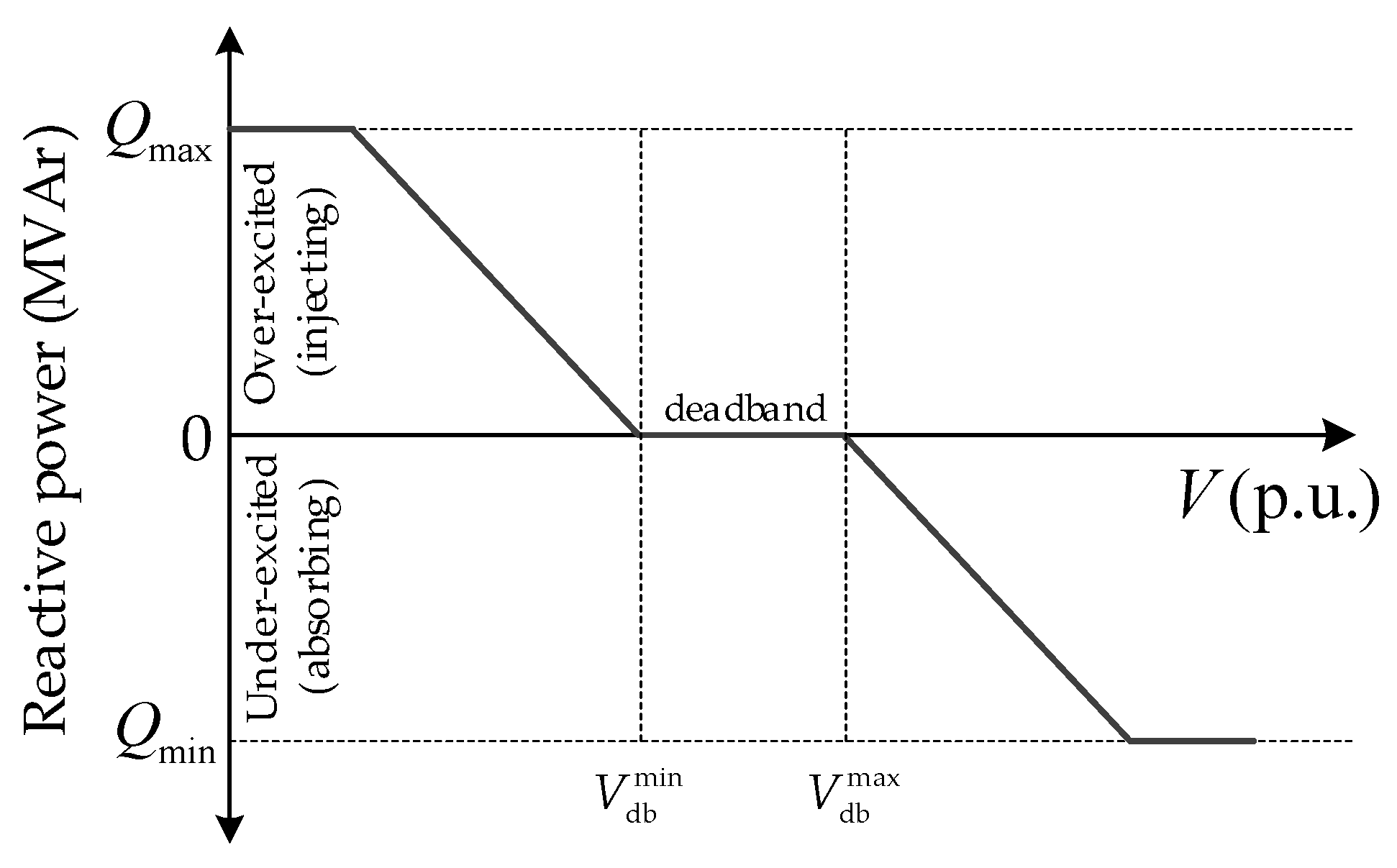
2.6. Voltage-Reactive Power Control (Volt-Var)

The Volt-Var control is based on a piecewise linear Q(V)-characteristic, as shown in Figure 2. The smart inverter provides a constant value of reactive power when the voltage at the local bus is inside its maximum and minimum deadband values, i.e., Q_out = Q_target ∀ V ∈ [V^min_db, V^max_db]. Otherwise, if the voltage leaves the deadband zone, the reactive power output of the smart inverter is determined by the actual voltage and the slope of the Q(V)-characteristic.

2.7. Constant Power Factor Control (Constant ϕ)

The power factor of the smart inverter is kept constant by adjusting the reactive power output according to the active power output (P_out). Therefore, the resulting reactive power output is computed as:

$$Q_{\mathrm{out}}=P_{\mathrm{out}}{\tan }^{-1}\left({\cos }^{-1}\varphi \right)$$

(3)

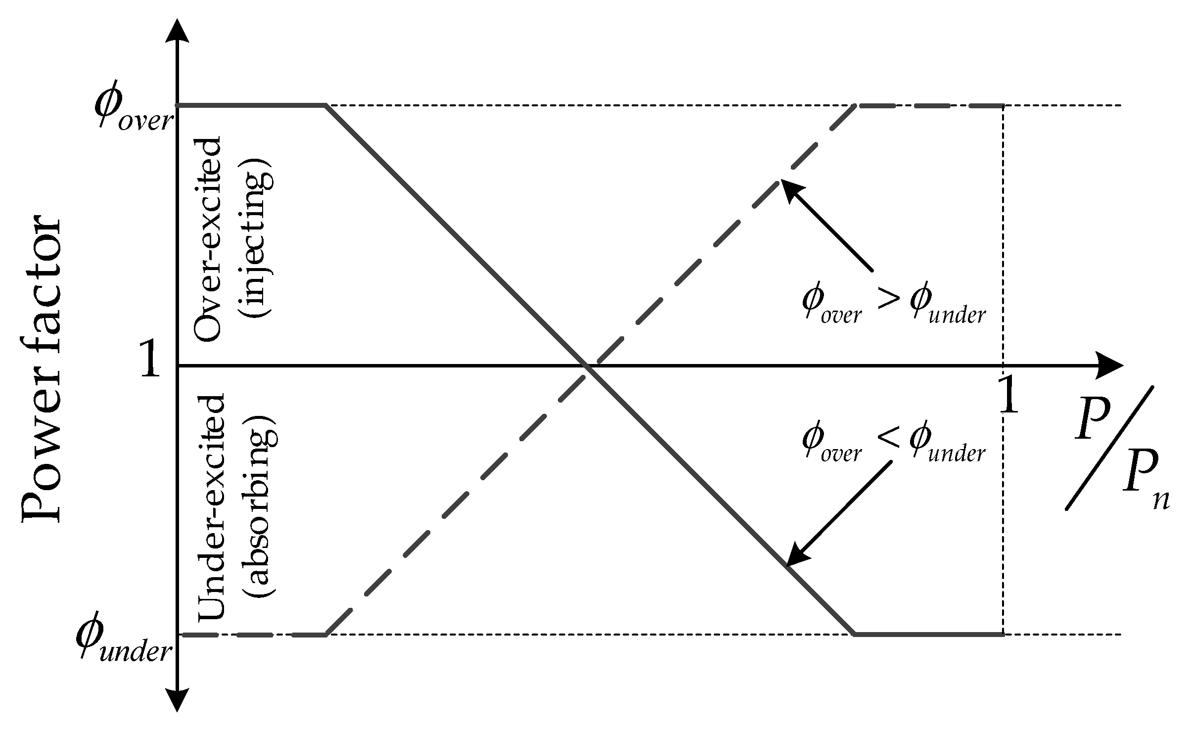
2.8. Power Factor-Active Power-Based Control (ϕ−Watt)

The smart inverter controls the reactive power output by adjusting the power factor according to the active power output and the piecewise linear ϕ (P)−characteristic shown in Figure 3.

Further information on the main features of each reactive power control strategy is addressed in [14,15].

Smart inverters have been used extensively in renewable integration, and their smart functions have been demonstrated to enhance the response and power capability when tie-grid connected. An example of such enhancement is the PV interconnection shown in [16], presenting one of the most advantages of the smart inverters, the voltage rise (Volt-Var) in the distribution network operation. Therefore, solar farms are interconnected through a smart inverter to support the grid with different ancillary services and allow appropriate management of the sources [17]. Additionally, smart inverters are used in wind farms interconnection for providing several grid services, including reactive power support [18]. This grid service has become a standard for manufacturers and wind power developers since the grid codes require being included since the grid is drastically changing with the continuous expansion and the incorporation of more DER.

Although smart inverter functionalities are contributing to the RES interconnection, it is necessary to meditate about the international and national standards, guidelines, technical reports regarding the impact of the smart inverters on the interaction between the smart inverters and their elements. An example of this interaction is studied in [19], emphasising the multiple standards required for the grid interconnection correlated to the smart functionalities.

3. Optimum Reactive Power Control at Smart Inverters

The main reason to seek suitable reactive power control mechanisms is to provide voltage support and ensure voltage stability. However, an increase in the active power losses and/or deterioration of the voltage profile may be produced if the amount of reactive power injection/absorption supplied by the smart inverter is not adequate. Therefore, besides the eight reactive power control mechanisms described in Section 2, an optimum reactive power (ORP) control proposed in this paper is evaluated. The main goal of this control is to minimise the active power losses in the network while ensuring all busbar voltages are inside the safe operational limits and the reactive power limits of the smart inverter are enforced.

The total active power loss (P_loss) of the network is calculated as the difference between the total power generation (P_g) and the total power demand (P_d) as follows:

$$P_{\mathrm{loss}}=P_g-P_d$$

(4)

The objective function to minimise P_loss is defined as:

$$\min P_{\mathrm{loss}}\left(Q\right)$$

(5)

subject to:

$$Q_{\min }<Q<Q_{\max }$$

(6)

where Q is the vector of controlled variables containing the reactive power output of the smart inverters, Q_min, and Q_max are vectors containing the minimum and maximum reactive power limits of the smart inverters, respectively.

The reactive power injected/absorbed by the smart inverters will directly influence the voltage profile. As a consequence, it is necessary to ensure voltages at all buses remains inside its allowable operational limits, and this is explicitly formulated as inequality constraints, rather than the use of penalty function, to guarantee the optimum solution. The set of voltage inequality constraints is

$$\left[\left|V_{\mathrm{n}}-V_i\right|-\Delta V\right]<0\forall i=1,2,\dots ,n_b$$

(7)

where V_n is the nominal voltage, V_i is the voltage at the i-th bus, ∆V is the permissible voltage deviation (usually ±5% of the nominal voltage), and n_b represents the number of buses in the network.

4. Cost of Reactive Power Provision by Smart Inverters

The reactive power procurement services vary depending on the different deregulated markets. Moreover, they do not have an established structure in contrast with the active power market, which has a recognised mechanism for pricing. Currently, there is no evidence of reactive power services procurement by using a competitive approach. A few countries such as the USA, Great Britain, and Australia provide monetary compensation for reactive power services coming from the synchronous generator. Meanwhile, in Nordic countries and Germany, reactive power services are not compensated. In general, at the transmission level, the reactive power needs are covered by special tenders; meanwhile, at the distribution level, the reactive power is controlled by limiting the power factor value of the DERs [20].

Due to there is not a mechanism for the reactive power procurement and pricing, in this paper, the cost of the reactive power services provided by the smart inverters is determined following the non-mandatory enhancement reactive power service (ERPS) regulation established by the National Grid [21]. Therefore, the price of the reactive power (γ) is taken from the default payment rate document [22], for August 2020, which is γ = 2.337227 £/MVAr.

Assuming the daily steady-state of the network is discretised in periods of T minutes over 24 h, the daily cost of reactive power services in steady-state is computed using the following equation:

$$C_Q=\frac{1}{n_T}{\displaystyle \sum _{j=1}^{N_T}{Q}_{\mathrm{SI},}{}_j}{\gamma }_j$$

(8)

where Q_SI,j is the total reactive power at the point common connection delivered by the smart inverters, and γ_j is the price of the reactive power in the j-th period. Moreover, n_T is the number of periods per hour, and N_T is the total number of periods over 24 h.

5. Results

This section is dedicated to describing the test system employed to assess the reactive power control mechanisms enabled at the PVs, in addition to defining the study cases considered in this paper and presenting the main results and findings.

5.1. Test System

The eight reactive power control mechanisms and the proposed ORP control described in Section 2 and Section 3, respectively, are assessed using the Vestfold and Telemark (V&T) distribution network of the south-eastern area of Norway shown in Figure 4. The V&T distribution network is interconnected with the Norwegian power system through 300 and 420 kV transmission lines and consists of 20 hydropower plants and 58 loads (eight residential and 50 industrial) [8]. It has been implemented using DIgSILENT PowerFactory and was equipped with 58 solar PV based smart inverters installed on the load buses. The load profile and solar PV profile representative of the daily operation, considering 15 min periods, were synthetically generated using the CREST tool [23,24]. The CREST tool was set up to include the temperature and location of the south-eastern area of Norway [2].

5.2. Study Cases

The assessment of the reactive power control mechanism is carried out by studying two scenarios: Scenario I considers a fixed price of reactive power over 24 h. Meanwhile, Scenario II considers a variable price curve based on the normalised total reactive power demand over 24 h. These two scenarios are evaluated considering nine cases; each case represents one reactive power control mechanism. The detailed definition of the nine cases and the parameters of each reactive power control mechanism are depicted in

Table 1. Study cases and parameters of the reactive power control mechanisms enabled at the PVs.

Case	Control Mechanism	Parameters
C.I	constant V	Vtarget = 1.00 pu.
C.II	Q-droop	KQ-droop = 10%, Vtarget,min = 0.98 pu, Vtarget,max = 1.02 pu.
C.III	Iq-droop	KIq-droop = 10%, Vtarget,min = 0.98 pu, Vtarget,max = 1.02 pu.
C.IV	constant Q	Q = Snsin (θ) @ ϕ = 0.9
C.V	Watt−Var	$Q_{\max ,k}=-Q_{\min ,k}=\sqrt{S_{n,k}^2-P_{n,k}^2}\forall k=1,2,\dots ,n_{PV}$
C.VI	Volt−Var	Vmindb = 0.99 pu, Vmaxdb = 1.01 pu. $Q_{\max ,k}=-Q_{\min ,k}=\sqrt{S_{n,k}^2-P_{n,k}^2}\forall k=1,2,\dots ,n_{PV}$
C.VII	constant ϕ	ϕ = 0.85
C.VIII	ϕ−Watt	ϕover = 0.95, ϕunder = 0.95
C.IX	ORP	∆V = 0.02 pu., $Q_{\max ,k}=-Q_{\min ,k}=\sqrt{S_{n,k}^2-P_{\mathrm{out},k}^2}\forall k=1,2,\dots ,n_{PV}$

The optimisation of the ORP control was solved using the improved harmony search algorithm, and its parameter were set up as [8,25]: HMS = 1, HMCR = 0.9, PAR_min = 0.35, PAR_max = 0.99, bw_min = 1 × 10⁻⁵, bw_max = 1.0 and improvisations = 1500. Moreover, Python programming language was used together with DIgSILENT PowerFactory to automate the simulations and to solve the optimisation problem.

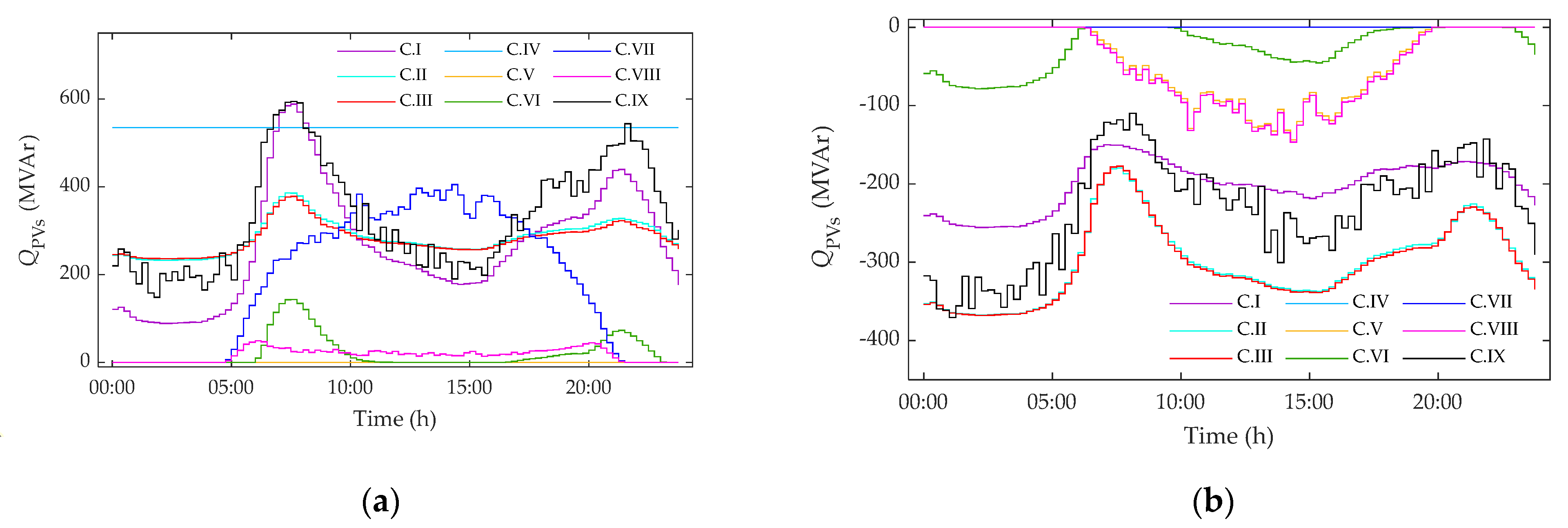
5.3. Results and Discussion

The nine cases of reactive power control defined in Table 1. were evaluated by performing the steady-state operation of the V&T distribution network considering 15 min periods over 24 h. The total reactive power injected and absorbed by the 58 solar-PVs installed in the V&T distribution network is presented in Figure 4. It can be observed that the Watt−Var control (C.V) leads to the PVs not supplying any reactive power, meaning that this control maintains PVs under-excited, and its power factor is capacitive (see Figure 5a). On the other hand, as the constant Q control (C.IV) and constant ϕ control (C.VII) were set to inductive power factor, they only inject reactive power (see Figure 5b). The remaining cases absorb and inject reactive power as required by the network.

The idea of a suitable reactive power control is that it be able to provide reactive power services to regulate the lack or excess of reactive power. Therefore, cases C.IV and C.VII are not suitable to provide reactive power services since they are not able to adapt as the power system requires a daily steady-state operation.

Assuming only the reactive power services of the PVs corresponding to the supplied reactive power are paid. The daily cost of reactive power is computed using (8). It is considered Scenario I, where the fixed price of reactive power is used and Scenario II, where the variable price of reactive power is utilised. The total daily cost of reactive power supplied by the PVs of the two scenarios, considering the nine cases of control, is presented in

Table 2. Daily cost of reactive power supplied by the solar PVs implementing the nine reactive power control mechanisms.

Case	CQ (£/Day)
	Scenario I	Scenario II
C.I	14,916.28	10,586.55
C.II	15,958.65	10,241.84
C.III	15,747.87	10,066.76
C.IV	30,001.09	18,500.32
C.V	0.00	0.00
C.VI	1207.83	1043.23
C.VII	10,429.49	7148.27
C.VIII	969.68	693.52
C.IX	18,694.48	12,730.06

.

From Table 2, it can be observed that implementing a variable price over the 24 h operations leads to reduce the total cost of the reactive power procured from the solar PVs around between 14% to 35% in contrast to use a fixed price. Therefore, focusing on Scenario II, which produces lower costs, the ϕ−Watt control (C.VIII) generates the lower cost of reactive power. The maximum cost is produced by constant Q control (C.IV), which had previously been determined as unsuitable control because it is not able to auto-adjust to operate in the under-excited and over-excited regions. Even though the ϕ−Watt control produces the lower cost for procuring reactive power, the technical and operational requirements must be evaluated to ensure its control has the best cost–benefit relationship. Therefore, the total energy losses and the minimum and maximum voltage over the 24 h for the nine reactive power control cases are presented in

Table 3. Daily energy losses and voltage resulting by implementing different reactive power control modes.

Case	Eloss (MW/day)	Voltage (pu)
		Minimum	Maximum
C.I	438.50	0.997	1.024
C.II	445.04	0.980	0.997
C.III	445.28	0.980	0.997
C.IV	518.63	0.995	1.125
C.V	456.42	0.930	1.058
C.VI	450.18	0.966	1.041
C.VII	469.52	0.959	1.098
C.VIII	456.15	0.932	1.058
C.IX	436.43	0.987	1.020

.

From Table 3, it can be observed the minimum daily energy loss is produced by the ORP control (C.IX); meanwhile, the maximum energy loss occurs using the constant Q control (C.IV). Moreover, for all control cases, the maximum allowable voltage variation was set as 0.02 pu. It means the bus voltages must be kept between V_min = 0.98 pu and V_max = 1.02 pu. However, only cases C.II, C.III, and C.IX met this technical requirement. Therefore, even though ORP control produces a cost 20% higher than C.II and C.III, it is the only one that meets up all technical requirements and produces the best cost–benefit relationship to the network.

6. Conclusions

The assessment of the cost–benefit relationship of the eight reactive power control mechanisms and the proposed optimum reactive power control demonstrates the best suitable reactive control is the optimum reactive power control. It optimally adjusts the reactive power injection absorption and ensures the technical requirements are fulfilled (voltage stability). Moreover, economically, it produces the minimum active power losses and generates considerable low reactive power costs in comparison with the other eight reactive power control mechanisms.

This assessment provides a new perspective to the TSO and DSO about the procurement of reactive power services from the DERs. It opens the door to start creating new reactive power market mechanisms that allow fair trade pricing the reactive power. Moreover, it reveals that in a reactive power procurement landscape, employing variable prices according to the need for reactive power in the network will reduce the daily cost of reactive power in contrast to using a fixed price over 24 h.

References

1. Gonzalez-Longatt, F.; Acosta, M.N.; Chamorro, H.R.; Rueda, J.L. Power Converters Dominated Power Systems. In Modelling and Simulation of Power Electronic Converter Controlled Power Systems in Power Factory; Gonzalez-Longatt, F., Rueda, J.L., Eds.; Springer Nature Switzerland AG: Cham, Switzerland, 2020. [Google Scholar]
2. Pettersen, D.; Melfald, E.; Chowdhury, A.; Acosta, M.N.; Gonzalez-Longatt, F.; Topic, D. TSO-DSO Performance Considering Volt-Var Control at Smart-Inverters: Case of Vestfold and Telemark in Norway. In Proceedings of the 2020 International Conference on Smart Systems and Technologies (SST), Osijek, Croatia, 14–16 October 2020; pp. 147–152. [Google Scholar]
3. Gonzalez-Longatt, F.; Acosta, M.N.; Chamorro, H.R.; Topic, D. Short-term Kinetic Energy Forecast using a Structural Time Series Model: Study Case of Nordic Power System. In Proceedings of the 2020 International Conference on Smart Systems and Technologies (SST), Osijek, Croatia, 14–16 October 2020; pp. 173–178. [Google Scholar]
4. Krechel, F.T.; Sanchez, F.; Gonzalez-Longatt, H.C.; Rueda, J.L. Transmission System Friendly Micro-grids: An option to provide Ancillary Services. In Distributed Energy Resources in Microgrids; Chauhan, R.K., Chauhan, K., Eds.; Elsevier: Amsterdam, The Netherlands, 2018. [Google Scholar]
5. Ersdal, A.M.; Gonzalez-Longatt, F.; Acosta, M.N.; Rueda, J.L.; Palensky, P. Frequency Support of Fast-Multi-Energy Storage Systems in Low Rotational Inertia Scenarios. In Proceedings of the 2020 IEEE PES Innovative Smart Grid Technologies Europe (ISGT-Europe), The Hague, The Netherlands, 26–28 October 2020; pp. 879–883. [Google Scholar]
6. Krechel, T.; Sanchez, F.; Gonzalez-Longatt, F.; Chamorro, H.R.; Rueda, J.L. A Transmission System Friendly Micro-grid: Optimising Active Power Losses. In Proceedings of the 2019 IEEE Milan Power Tech, Milan, Italy, 23–27 June 2019; pp. 1–6. [Google Scholar]
7. Sanchez, F.; Cayenne, J.; Gonzalez-Longatt, F.; Rueda, J.L. Controller to enable the enhanced frequency response services from a multi-electrical energy storage system. IET Gener. Transm. Distrib. 2019, 13, 258–265. [Google Scholar] [CrossRef] [Green Version]
8. Acosta, M.N.; Pettersen, D.; Gonzalez-Longatt, F.; Argos, J.P.; Andrade, M.A. Optimal Frequency Support of Variable-Speed Hydropower Plants at Telemark and Vestfold, Norway: Future Scenarios of Nordic Power System. Energies 2020, 13, 3377. [Google Scholar] [CrossRef]
9. Torkzadeh, R.; Chamorro, H.R.; Rye, R.; Eliassi, M.; Toma, L.; Gonzalez-Longatt, F. Reactive Power Control of Grid Interactive Battery Energy Storage System for WADC. In Proceedings of the 2019 IEEE PES Innovative Smart Grid Technologies Europe (ISGT-Europe), Bucharest, Romania, 29 September–2 October 2019; pp. 1–5. [Google Scholar]
10. IEEE Standard Association IEEE Std. 1547-2018. Standard for Interconnection and Interoperability of Distributed Energy Resources with Associated Electric Power Systems Interfaces; IEEE: Piscataway, NJ, USA, 2018; ISBN 9781504446396. [Google Scholar]
11. Demand Connection Code. Available online: https://www.entsoe.eu/network_codes/dcc/ (accessed on 13 October 2020).
12. Acosta, M.N.; Gonzalez-Longatt, F.; Denysiuk, S.; Strelkova, H. Optimal Settings of Fast Active Power Controller: Nordic Case. In Proceedings of the 2020 IEEE 7th International Conference on Energy Smart Systems (ESS), Kyiv, Ukraine, 12–14 May 2020; pp. 63–67. [Google Scholar]
13. Kaloudas, C.G.; Ochoa, L.F.; Marshall, B.; Majithia, S.; Fletcher, I. Assessing the Future Trends of Reactive Power Demand of Distribution Networks. IEEE Trans. Power Syst. 2017, 32, 4278–4288. [Google Scholar] [CrossRef] [Green Version]
14. Acosta, M.; Gonzalez-Longatt, F.; Topić, D.; Andrade, M. Optimal Microgrid–Interactive Reactive Power Management for Day–Ahead Operation. Energies 2021, 14, 1275. [Google Scholar] [CrossRef]
15. Zhao, X. Power System Support Functions Provided by Smart Inverters—A Review. CPSS Trans. Power Electron. Appl. 2018, 3, 25–35. [Google Scholar] [CrossRef]
16. Kikusato, H.; Ustun, T.S.; Hashimoto, J.; Otani, K. Aggregate Modeling of Distribution System with Multiple Smart Inverters. In Proceedings of the 2019 International Conference on Smart Energy Systems and Technologies (SEST), Porto, Portugal, 9–11 September 2019; pp. 1–6. [Google Scholar]
17. Varma, R.K.; Siavashi, E.M. Enhancement of Solar Farm Connectivity with Smart PV Inverter PV-STATCOM. IEEE Trans. Sustain. Energy 2019, 10, 1161–1171. [Google Scholar] [CrossRef]
18. Ouyang, J.; Tang, T.; Yao, J.; Li, M. Active Voltage Control for DFIG-Based Wind Farm Integrated Power System by Coordinating Active and Reactive Powers Under Wind Speed Variations. IEEE Trans. Energy Convers. 2019, 34, 1504–1511. [Google Scholar] [CrossRef]
19. Smolenski, R.; Jarnut, M.; Benysek, G.; Kempski, A. Power electronics interfaces for low voltage distribution generation EMC issues. In Proceedings of the 2011 7th International Conference-Workshop Compatibility and Power Electronics (CPE), Tallinn, Estonia, 1–3 June 2011; pp. 107–112. [Google Scholar]
20. Safari, A.; Salyani, P.; Hajiloo, M. Reactive power pricing in power markets: A comprehensive review. Int. J. Ambient. Energy 2020, 41, 1548–1558. [Google Scholar] [CrossRef]
21. Obligatory Reactive Power Service Default Payment Rates. Available online: https://data.nationalgrideso.com/backend/dataset/7e142b03-8650-4f46-8420-7ce1e84e1e5b/resource/e2e6f74c-ebca-48b3-b2ae-e4652d296dca/download/reactive-default-payment-rate-nov-2020.pdf (accessed on 19 October 2020).
22. Elexon. Available online: https://www.bmreports.com/bmrs/?q=balancing/systemsellbuyprices/historic (accessed on 22 September 2020).
23. Sanchez, F.; Gonzalez-Longatt, F.; Rodriguez, A.; Rueda, J.L. Dynamic Data-Driven SoC Control of BESS for Provision of Fast Frequency Response Services. In Proceedings of the 2019 IEEE Power & Energy Society General Meeting (PESGM), Atlanta, GA, USA, 4–8 August 2019; pp. 1–5. [Google Scholar] [CrossRef]
24. González-Longatt, F.; Carmona-Delgado, C.; Riquelme, J.; Burgos, M.; Rueda, J.L. Risk-based DC security assessment for future DC-independent system operator. In Proceedings of the 2015 International Conference on Energy Economics and Environment (ICEEE), Greater Noida, India, 27–28 March 2015; pp. 1–8.
25. Improved Harmony Search (IHS)—Pagmo 2.15.0 Documentation. Available online: https://esa.github.io/pagmo2/docs/cpp/algorithms/ihs.html#_CPPv4N5pagmo3ihsE (accessed on 13 March 2020).
Figure 1. Smart inverter control based on Q(P)−characteristic.
Energies 14 04834 g001
Figure 2. Smart inverter control based on Q(V)−characteristic.
Energies 14 04834 g002
Figure 3. Smart inverter control based on ϕ (P)characteristic.
Energies 14 04834 g003
Figure 4. One-line diagram of the Vestfold and Telemark distribution network [2].
Energies 14 04834 g004
Figure 5. Total reactive power supplied by solar PVs every 15 min for the nine cases of reactive power control: (a) injection and (b) absorption.
Energies 14 04834 g005