
A Reference Thermal-Hydrologic-Mechanical Native State Model of the Utah FORGE Enhanced Geothermal Site


Abstract
:
1. Introduction
1.1. Overview of the Geologic Model
1.2. Modeling and Simulation Overview
1.2.1. FracMan
1.2.2. FALCON
2. Native State Modeling
2.1. Model Location and Dimensions
- To avoid lateral groundwater flow in the near surface sediments originating from the east side of the Opal Mound Structure (the southeast side of the model domain). Little data area available regarding the near surface flow system, but given the near surface temperature distributions, significant lateral flow is likely. This area is of little interest to the present study.
- To avoid the unsaturated portions of the near surface sediments. As we are simulating the system in a fully-coupled thermal-hydrologic-mechanical numerical framework, including the unsaturated zone has practical, and significant, implications for the computational burden and applicability of the equations of state at negative (capillary) pressures. None of these issues are insurmountable, but at the present time, the effort required to overcome them cannot be justified for an area of the site that is not of interest to the present study.
- To facilitate establishment of the stress boundary condition on the top model surface and aid in the calibration of the vertical stress in the model. The use of the Leapfrog Geothermal earth modeling package [28] (see below) allowed for summation of the saturated and unsaturated sediment column above the model domain and applying this as a overburden load on the top of the model domain. This enabled the evaluation of the grain density of the overlying sediments required for model calibration.
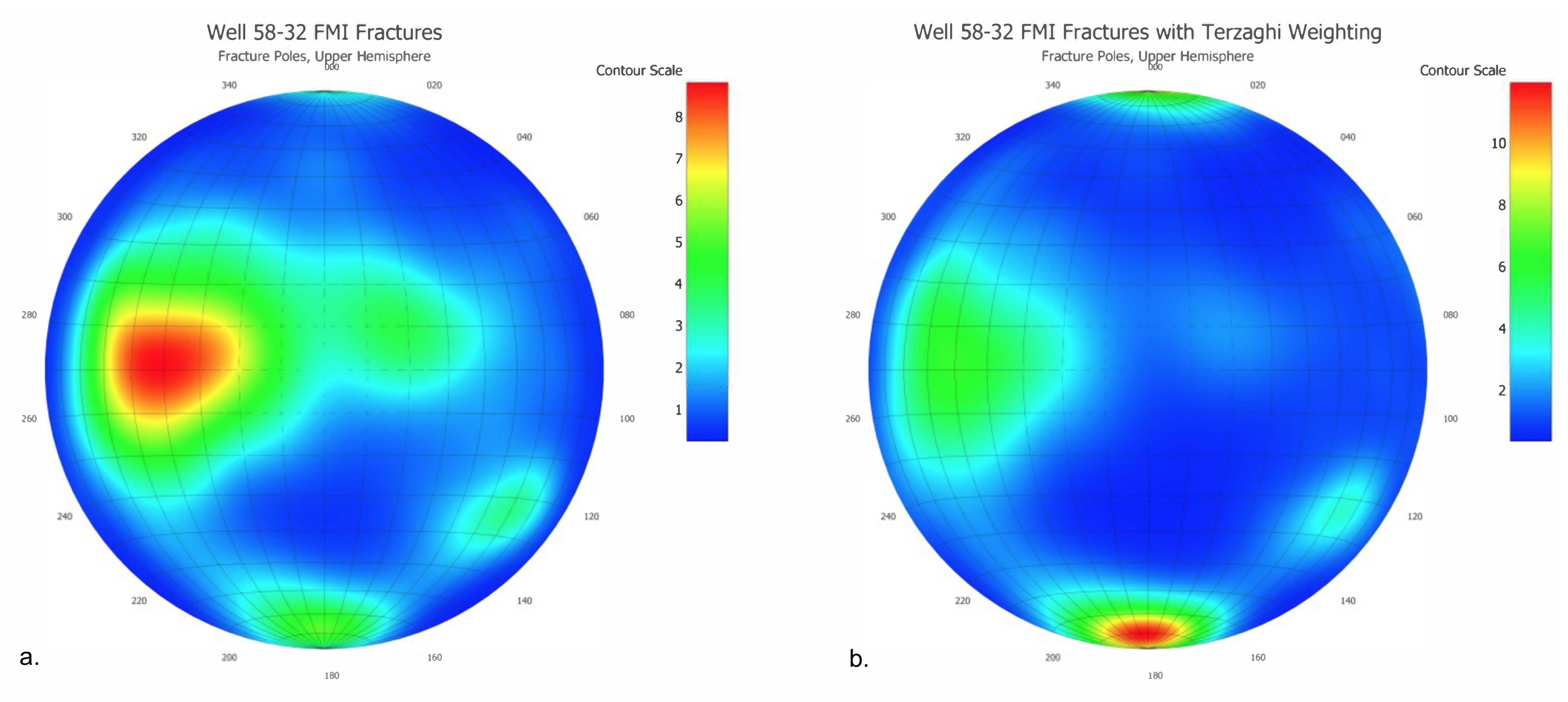
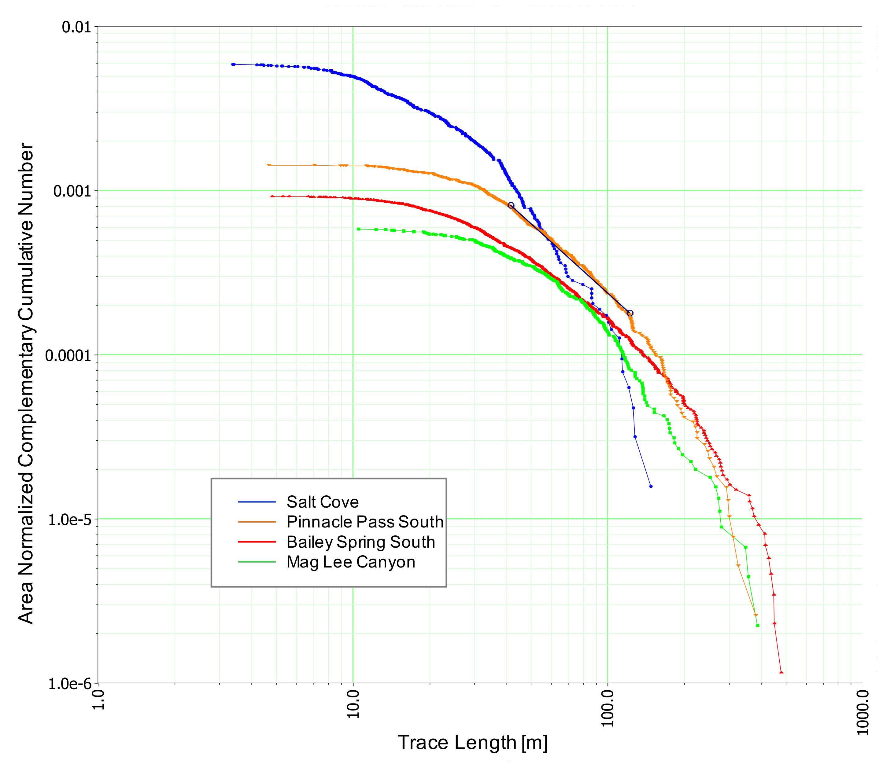
2.2. Reference Discrete Fracture Network
2.3. Rock and Fluid Properties
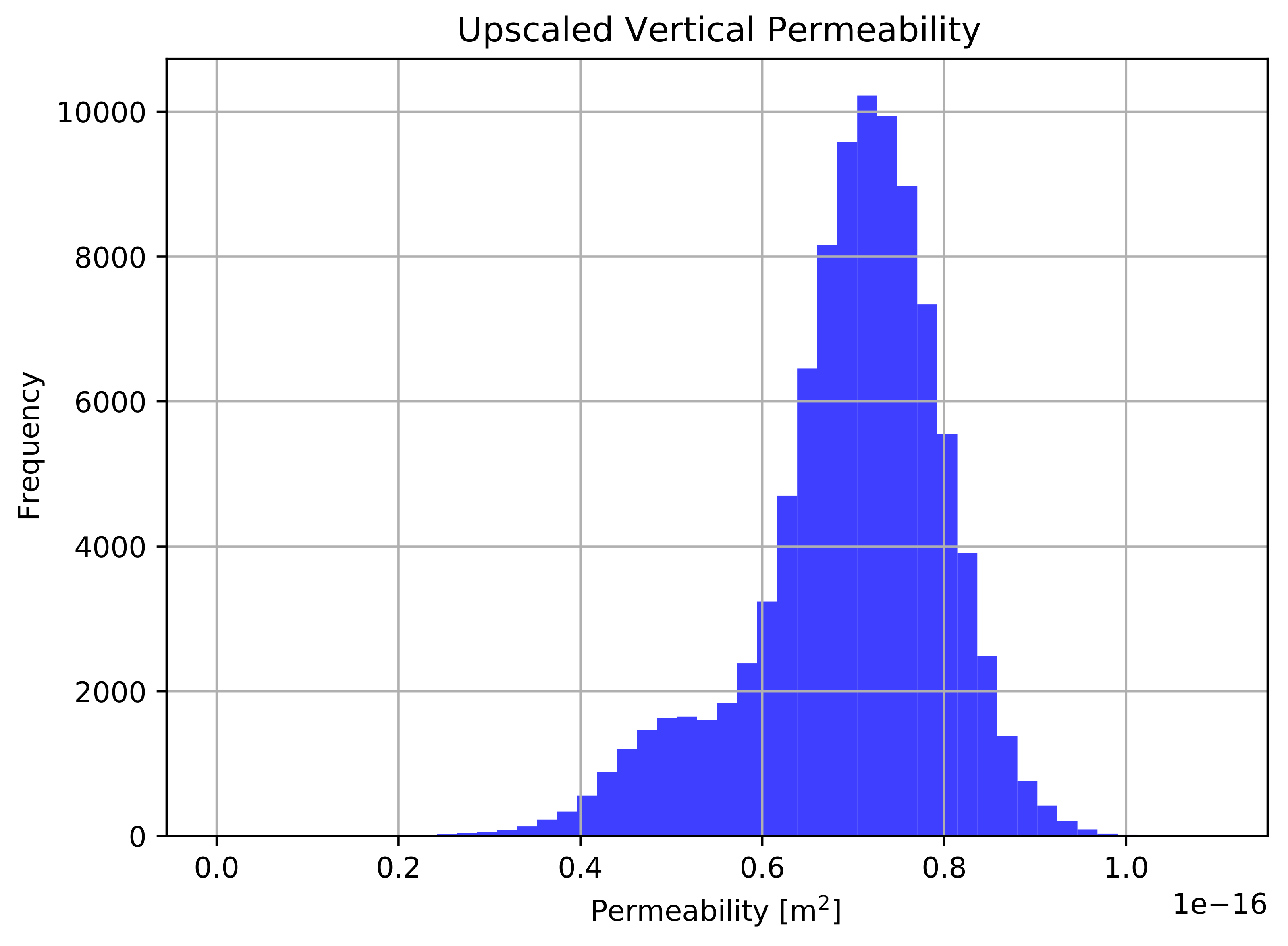
2.3.1. Hydrologic Properties
2.3.2. Thermal Properties
2.3.3. Mechanical Properties
2.3.4. Fluid Properties
- 273.15 K 1073.15 K, for 100 MPa;
- 1073.15 K 2273.15 K, for 50 MPa.
2.4. Boundary Conditions

| Parameter | Units | Min | Max | Source |
|---|---|---|---|---|
| Permeability | m | 6.9 × | 1.2 × | Upscaled DFN [29,51] Core-Reservoir testing [11] |
| Permeability | m | 4.5 × | 1.5 × | Upscaled DFN [29,51] Core-Reservoir testing [11] |
| Permeability | m | 6.2 × | 1.1 × | Upscaled DFN [29,51] Core-Reservoir testing [11] |
| Porosity | – | 1.0 × | 1.2 × | Upscaled DFN [29,51] Core-Reservoir testing [11] |
| Specific Heat Capacity | J kg K | 7.90 × | Cuttings analysis [38] Literature [52] Model calibration | |
| Grain Thermal Conductivity | W m K | 3.05 | Cuttings analysis [38] Model calibration | |
| Thermal Expansion Coefficient | K | 6.00 × | Literature [39] | |
| Rock Grain Density | kg m | 2.75 × | Core-cuttings analysis [11] Model calibration | |
| Young’s Modulus | Pa | 6.2 × | Core testing [11] | |
| Poisson’s Ratio | – | 0.30 | Core testing [11] | |
| Biot Coefficient | – | 0.60 | Literature [41] | |
| Parameter | Units | Value | Source |
|---|---|---|---|
| Permeability | m | 1.7 × | Aquifer testing [11] |
| Porosity | – | 1.2 × | Aquifer testing [11] Model calibration |
| Specific Heat Capacity | J kg K | 8.30 × | Literature [52] |
| Grain Thermal Conductivity | W m K | 2.0 | Cuttings analysis [38] Model calibration |
| Thermal Expansion Coefficient | K | 2.00 × | Literature [40] |
| Rock Grain Density | kg m | 2.50 × | Cuttings analysis [11] Model calibration |
| Young’s Modulus | Pa | 3.0 × | Literature [42] |
| Poisson’s Ratio | – | 0.30 | Literature [43] |
| Biot Coefficient | – | 0.60 | Literature [44] |
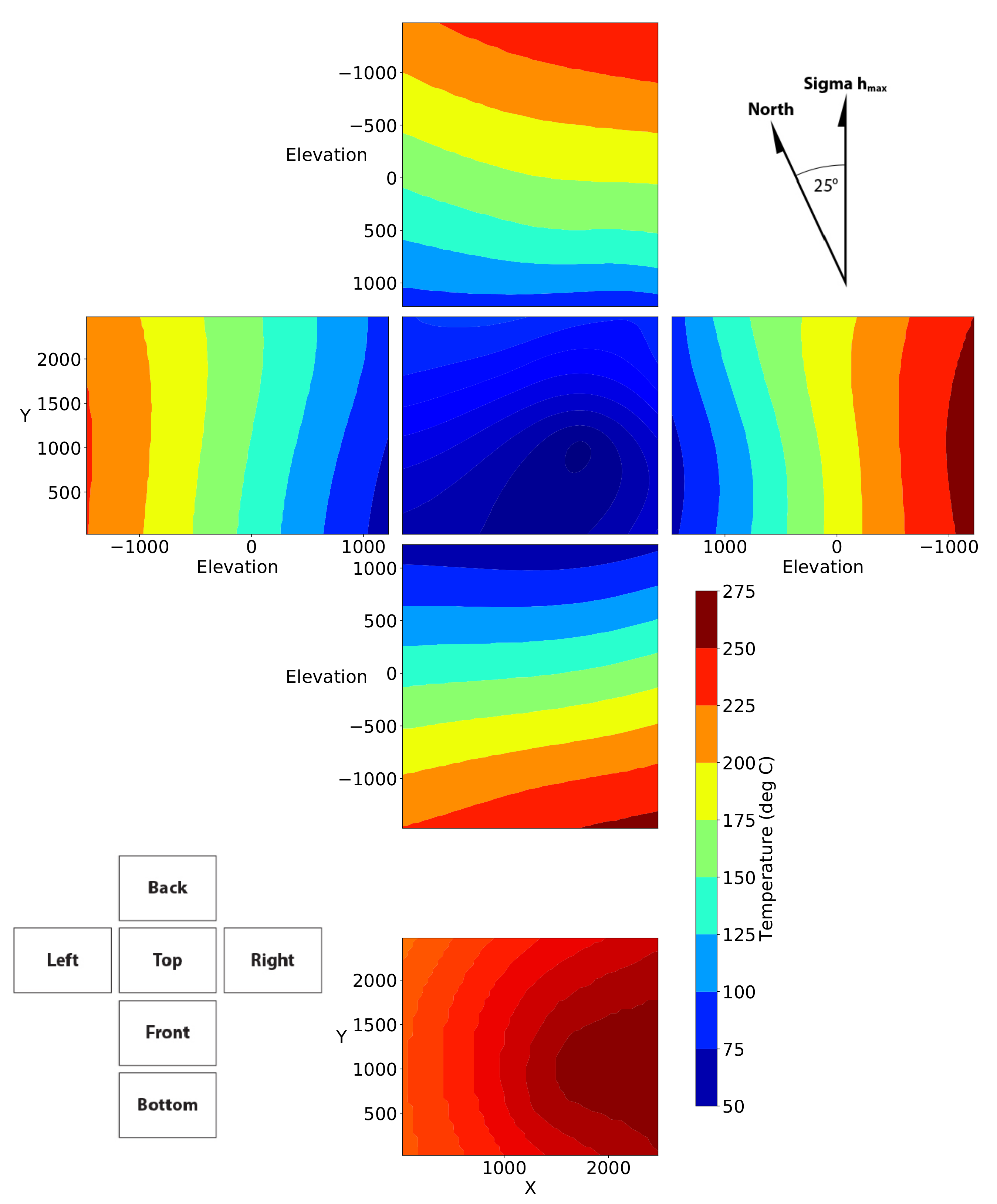
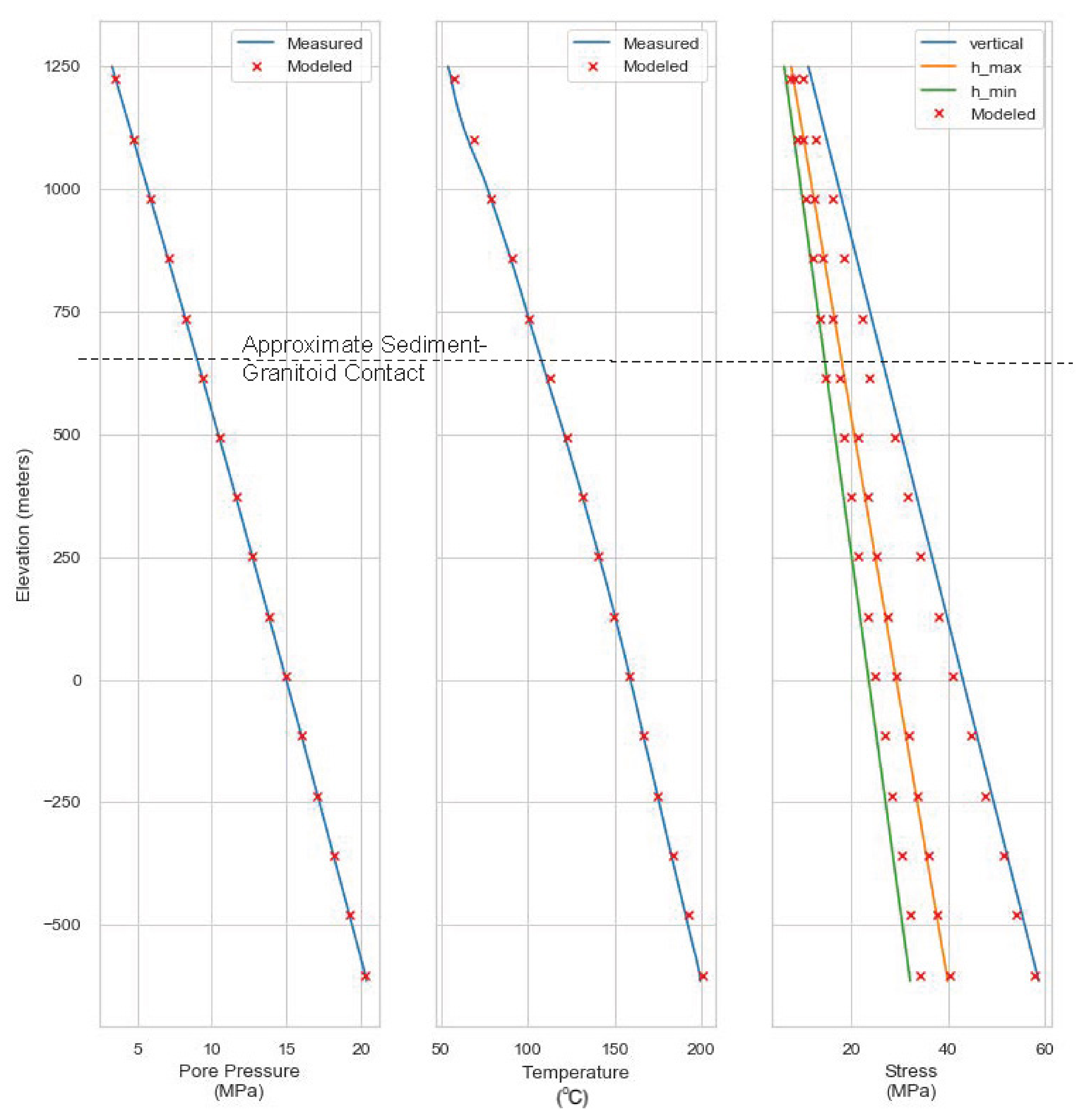
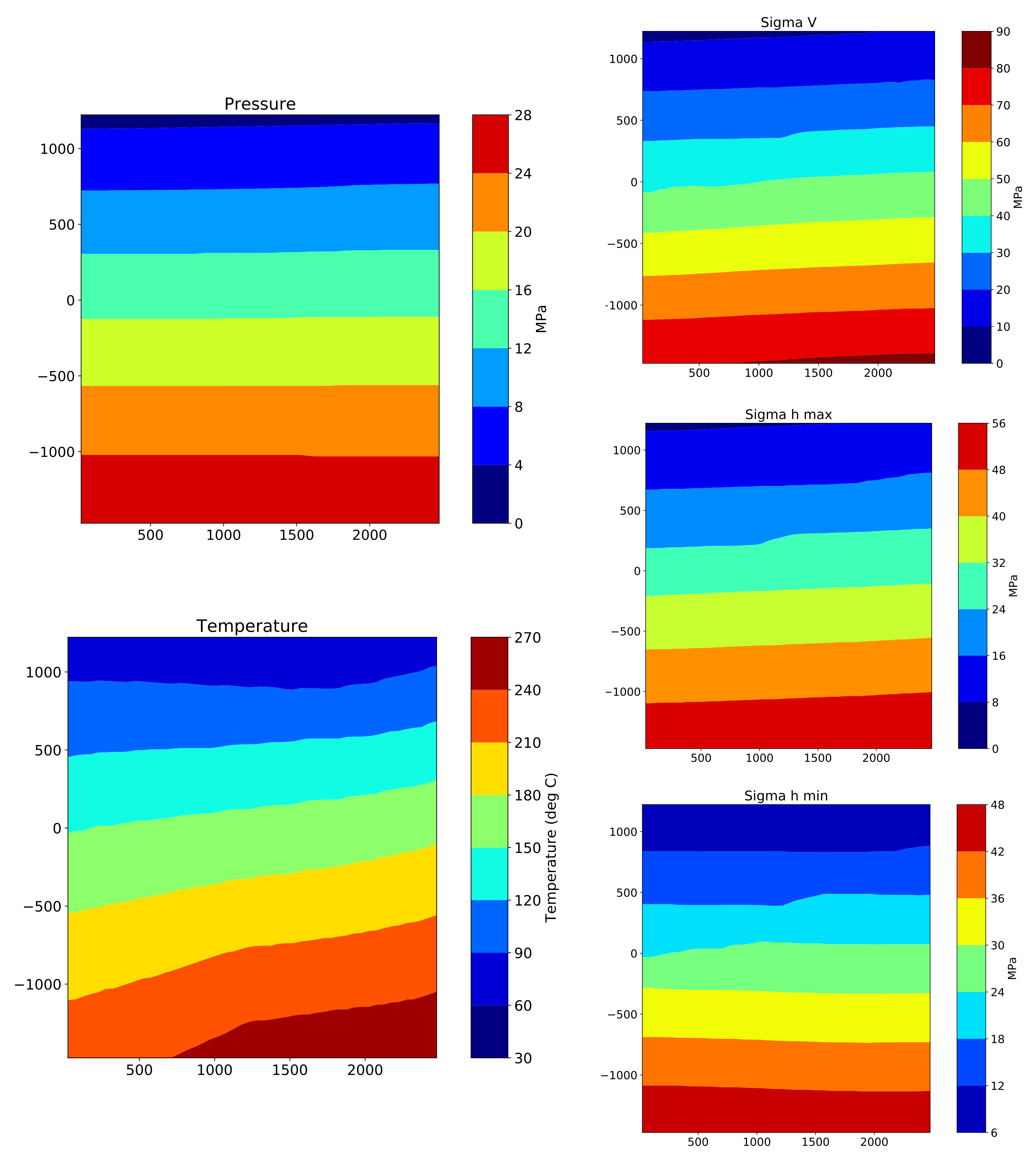
2.4.1. Temperature
2.4.2. Pressure
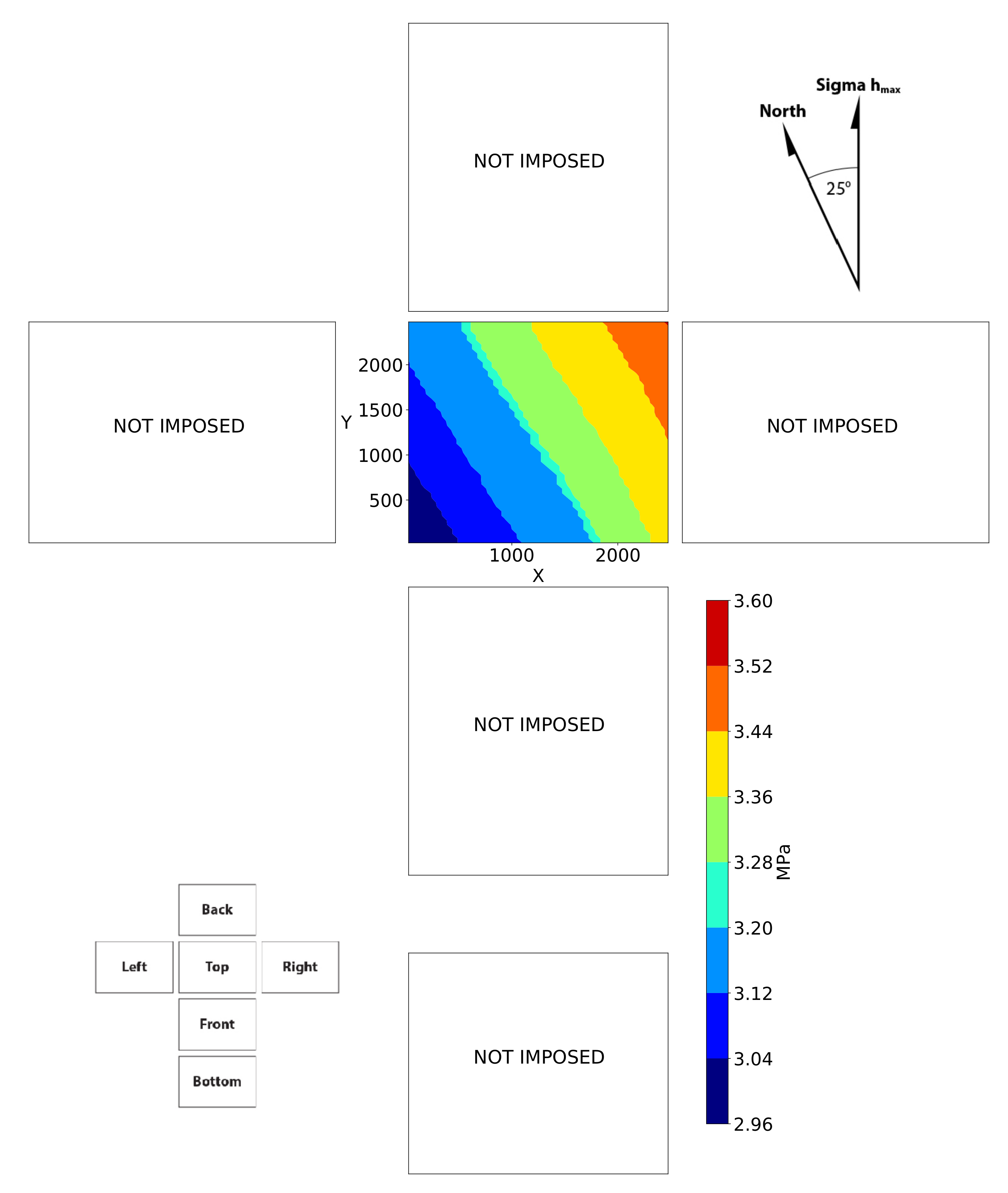
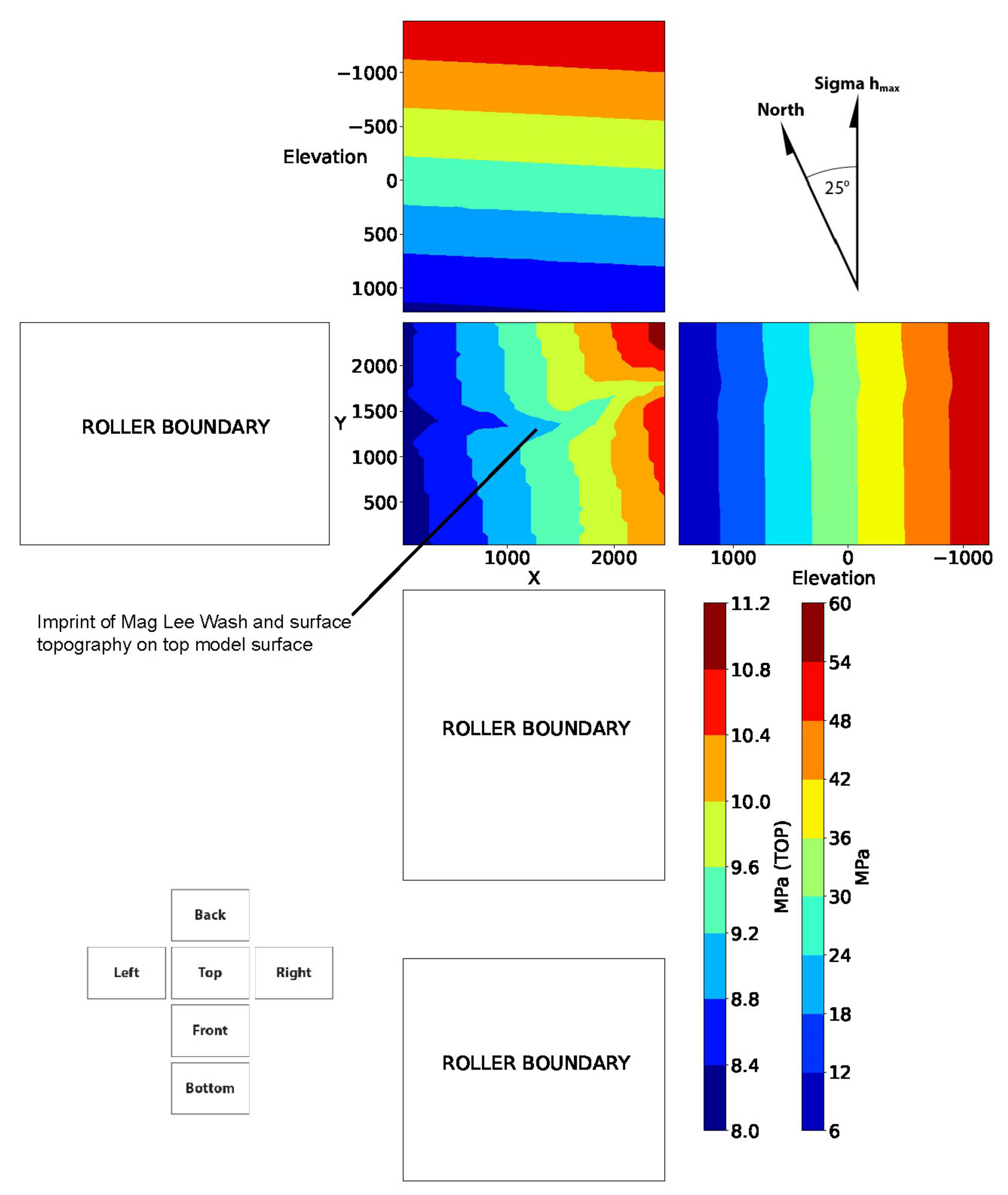
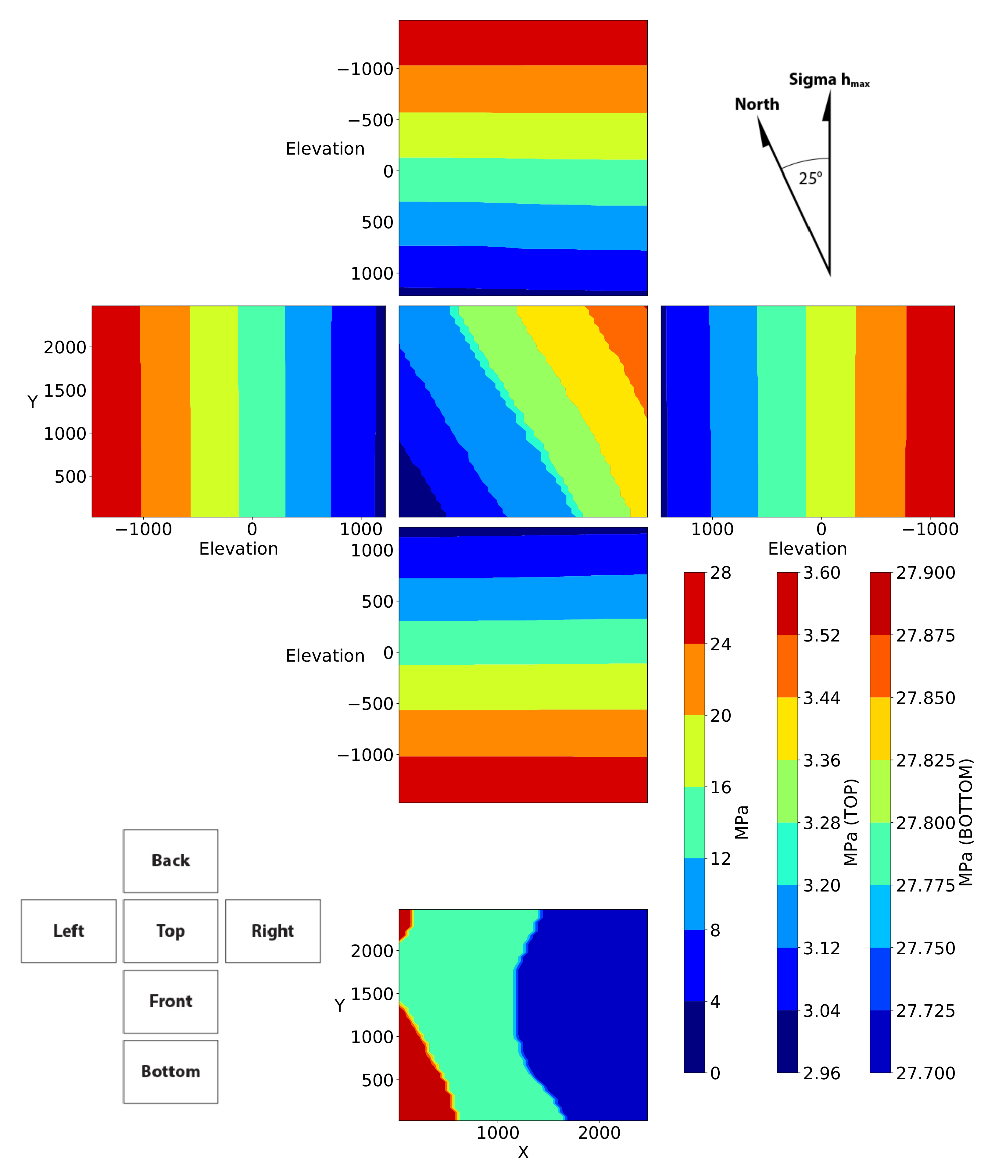
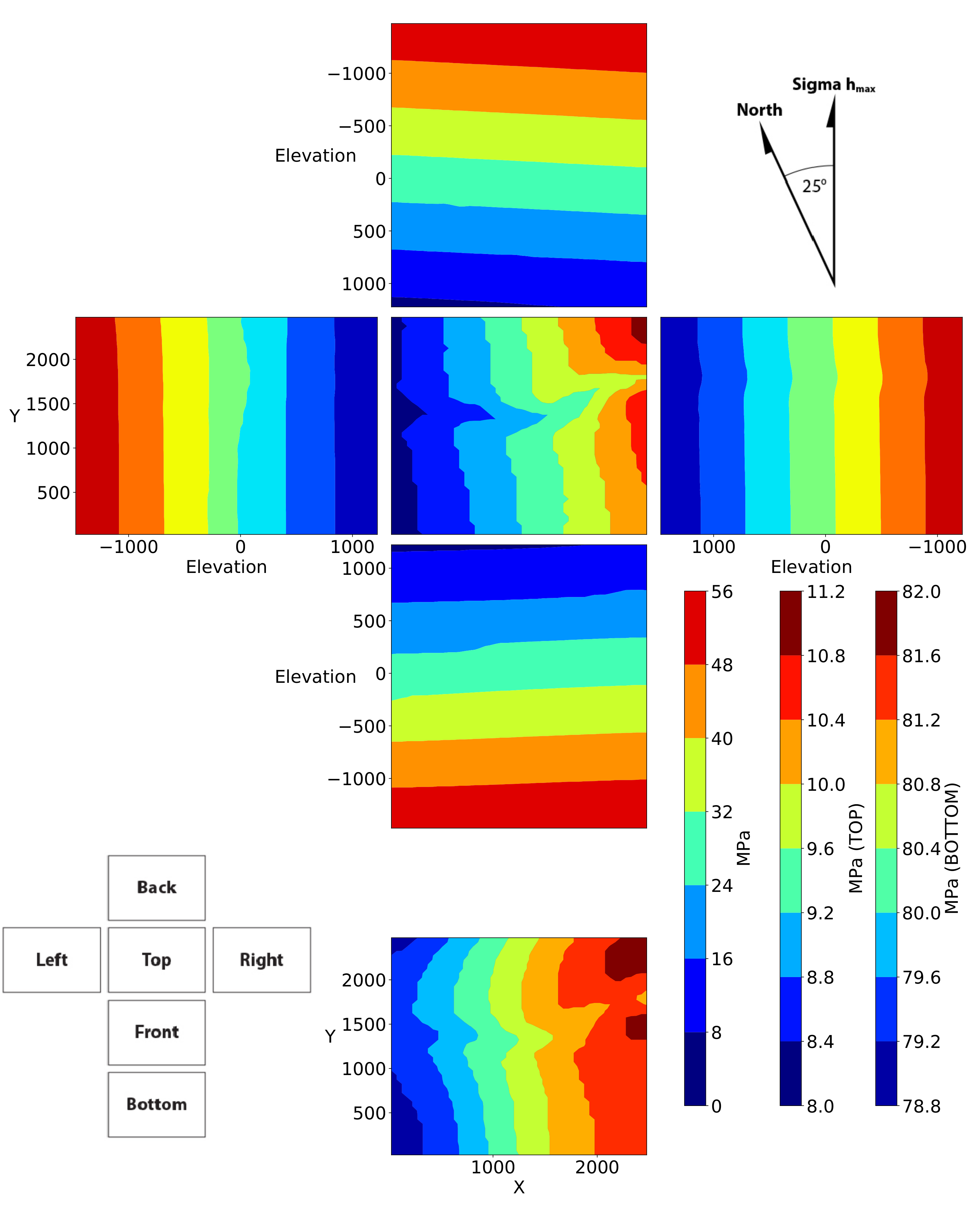
2.4.3. Stress
2.5. Initial Conditions
3. Results
4. Summary and Conclusions
Author Contributions
Funding
Data Availability Statement
Acknowledgments
Conflicts of Interest
References
- Batchelor, A.S. The Creation of Hot Dry Rock Systems by Combined Explosive and Hydraulic Fracturing. In Proceedings of the International Conference on Geothermal Energy, Florence, Italy, 11–14 May 1982; pp. 321–342. [Google Scholar]
- Cornet, F.H. Experimental Investigations of Forced Fluid Flow through a Granite Rock Mass. In Proceedings of the 4th International Seminar on the Results of EC Geothermal Energy Demonstration, Florence, Italy, 27–30 April 1989; pp. 189–204. [Google Scholar]
- Smith, M.C.; Aamodt, R.L.; Potter, R.M.; Brown, D.W. Manmade Geothermal Reservoirs; Technical Report LA-UR-75-953; Los Alamos National Laboratory: Los Alamos, NM, USA, 1975. [Google Scholar]
- Tester, J.W.; Brown, D.W.; Potter, R.M. Hot Dry Rock Geothermal Energy—A New Energy Agenda for the 21st Century; Technical Report LA-11514-MS; Los Alamos National Laboratory: Los Alamos, NM, USA, 1989. [Google Scholar]
- Duchane, D. Hot Dry Rock: A Realistic Energy Option. Bull. Geotherm. Resour. Counc. 1990, 19, 83–88. [Google Scholar]
- Duchane, D.; Brown, D. Hot Dry Rock (HDR) Geothermal Energy Research and Development at Fenton Hill, New Mexico. Geotherm. Heat Cent. Bull. 2002, 23, 13–19. [Google Scholar]
- Augustine, C. Update to enhanced geothermal system resource potential estimate. Geotherm. Resour. Counc. Trans. 2016, 40, 673–677. [Google Scholar]
- Tester, J.; Anderson, B.; Batchelor, A.; Blackwell, D.; DiPippo, R.; Drake, E.; Garnish, J.; Livesay, B.; Moore, M.; Nichols, K.; et al. The Future of Geothermal Energy: Impact of Enhanced Geothermal Systems (EGS) on the United States in the 21st Century; Technical Report INL/EXT-06-11746; Idaho National Laboratory: Idaho Falls, ID, USA, 2006. [Google Scholar]
- U.S. Department of Energy. GeoVision: Harnessing the Heat Beneath Our Feet; Technical Report; US Department of Energy: Washington, DC, USA, 2019.
- Kirby, S.M. Revised mapping of bedrock geology adjoining the Utah FORGE site. In Geothermal characteristics of the Roosevelt Hot Springs System and Adjacent FORGE EGS Site, Milford, Utah: Utah Geological Survey Miscellaneous Publication 169; Allis, R., Moore, J., Eds.; Utah Geological Survey: Salt Lake City, UT, USA, 2019; p. 6. [Google Scholar] [CrossRef]
- Moore, J.; Allis, R.; Simmons, S.; Nash, G.; McLennan, J.; Forbes, B.; Jones, C.; Pankow, K.; Hardwick, C.; Gwynn, M.; et al. Utah FORGE: Final Phase 2B Topical Report; Technical Report, DOE Geothermal Data Repository; Energy and Geoscience Institute at the University of Utah: Salt Lake City, UT, USA, 2018. [Google Scholar]
- Podgorney, R.; Finnila, A.; McLennan, J.; Ghassemi, A.; Huang, H.; Forbes, B.; Elliot, J. A framework for modeling and simulation of the Utah FORGE site. In Proceedings of the 44th Workshop on Geothermal Reservoir Engineering, Stanford, CA, USA, 11–13 February 2019. [Google Scholar]
- Nielson, D.L.; Evans, S.H.; Sibbett, B.S. Magmatic structural, and hydrothermal evolution of the Mineral Mountains intrusive complex, Utah. Geol. Soc. Am. Bull. 1986, 97, 765–777. [Google Scholar] [CrossRef]
- Coleman, D.S.; Walker, J.D.; Bartley, J.M.; Hodges, K.V. Thermochronologic evidence of footwall deformation during extensional core complex development, Mineral Mountains, Utah. In The Geologic Transition, High Plateaus to Great Basin—A Symposium and Field Guide; Utah Geologic Association: Salt Lake City, UT, USA, 2001; Volume 78, pp. 155–168. [Google Scholar]
- Lipman, P.; Rowley, P.; Mehnert, H.; Evans, S.; Nash, B.; Brown, F. Pleistocene rhyolite of the Mineral Mountains, Utah–Geothermal and archaeological significance. U. S. Geol. Surv. J. Res. 1978, 6, 133–147. [Google Scholar]
- Knudsen, T.; Kleber, E.; Hiscock, A.; Kirby, S. Quaternary Geology of the Utah FORGE Site and Vicinity, Millard and Beaver Counties, Utah; Technical Report Miscellaneous Publication 169-B; Utah Geological Survey: Salt Lake City, UT, USA, 2019. [Google Scholar]
- Podgorney, R.; McLennan, J. Utah FORGE: Well 58-32 Injection Test Data; Technical Report, DOE Geothermal Data Repository; Idaho National Laboratory: Idaho Falls, ID, USA, 2018. [Google Scholar]
- Podgorney, R.; Allis, R. Utah FORGE: Roosevelt Hot Springs Analytical Well-Based Temperature Model Data; Technical Report, DOE Geothermal Data Repository; Idaho National Laboratory: Idaho Falls, ID, USA, 2018. [Google Scholar]
- Podgorney, R.; McLennan, J.; Moore, J.; Simmons, S.; Wannamaker, P.; Allis, R.; Jones, C. Utah FORGE: Well Data for Student Competition; Technical Report, DOE Geothermal Data Repository; Idaho National Laboratory: Idaho Falls, ID, USA, 2018. [Google Scholar]
- Podgorney, R.; McLennan, J.; Simmons, S.; Moore, J.; Allis, R.; Hill, J.; Hartwick, C. Utah FORGE: Maps and GIS Data from the Earth Model; Technical Report, DOE Geothermal Data Repository; Idaho National Laboratory: Idaho Falls, ID, USA, 2018. [Google Scholar]
- Podgorney, R. Utah FORGE: Earth Model Mesh Data for Selected Surfaces; Technical Report, DOE Geothermal Data Repository; Idaho National Laboratory: Idaho Falls, ID, USA, 2018. [Google Scholar]
- Golder Associates. FracMan Reservoir Edition Version 7.8 Discrete Fracture Network Simulator; Technical Report; Golder Associates: Redmomd, WA, USA, 2019. [Google Scholar]
- Podgorney, R.; Huang, H.; Lu, C.; Gaston, D.; Permann, C.; Guo, L.; Andrs, D. Falcon: A Physics-Based and Massively Parallel and Fully-Coupled, Finite Element Model for Simultaneously Solving Multiphase Fluid Flow, Heat Transport, and Rock Deformation for Geothermal Reservoir Simulation; Technical Report INL/EXT-11e23351; Idaho National Laboratory: Idaho Falls, ID, USA, 2014. [Google Scholar]
- Xia, Y.; Podgorney, R.; Huang, H. Assessment of a hybrid continuous/discontinuous Galerkin finite element code for geothermal reservoir simulations. Rock Mech. Rock Eng. 2016. [Google Scholar] [CrossRef]
- Xia, Y.; Podgorney, R. Falcon: Finite Element Geothermal Reservoir Simulation Code. Available online: https://mooseframework.inl.gov/falcon/ (accessed on 1 August 2021).
- Gaston, D.; Guo, L.; Hansen, G.; Huang, H.; Johnson, R.; Knoll, D.; Newman, C.; Park, H.K.; Podgorney, R.; Tonks, M.; et al. Parallel Algorithms and Software for Nuclear, Energy, and Environmental Applications Part I: Multiphysics Algorithms. Commun. Comput. Phys. 2012, 12, 807–833. [Google Scholar] [CrossRef]
- Gaston, D.; Guo, L.; Hansen, G.; Huang, H.; Johnson, R.; Knoll, D.; Newman, C.; Park, H.K.; Podgorney, R.; Tonks, M.; et al. Parallel Algorithms and Software for Nuclear, Energy, and Environmental Applications Part II: Multiphysics Software. Commun. Comput. Phys. 2012, 12, 834–865. [Google Scholar]
- Seequent. User Manual for Leapfrog Geothermal; Version 5; Seequent: Christchruch, New Zealand, 2020. [Google Scholar]
- Finnila, A.; Forbes, B.; Podgorney, R. Building and Utilizing a Discrete Fracture Network Model of the FORGE Utah Site. In Proceedings of the 44th Workshop on Geothermal Reservoir Engineering, Stanford, CA, USA, 11–13 February 2019; pp. 11–13. [Google Scholar]
- Terzaghi, R. Sources of error in joint surveys. Geotechnique 1965, 15, 287–304. [Google Scholar] [CrossRef]
- Dershowitz, W.S.; Herda, H.H. Interpretation of fracture spacing and intensity. In Proceedings of the 33rd U.S. Symposium on Rock Mechanics, Santa Fe, NM, USA, 3–5 June 1992. [Google Scholar]
- Dershowitz, W.; Ambrose, R.; Lim, D.; Cottrell, M. Hydraulic Fracture and Natural Fracture Simulation for Improved Shale Gas Development. In Proceedings of the Annual Conference and Exhibition Houston, Houston, TX, USA, 10–13 April 2011; American Association of Petroleum Geologists: Houston, TX, USA, 2011. [Google Scholar]
- Gwynn, M.; Allis, R.; Hardwick, C.; Jones, C.; Nielsen, P.; Hurlbut, W. Compilation of Rock Properties from Well 58-32, Milford, Utah FORGE Site, FORGE Utah; Technical Report; Energy and Geoscience Institute at the University of Utah: Salt Lake City, UT, USA, 2018. [Google Scholar]
- Bartley, J.M. Joint patterns in the mineral mountains intrusive complex and their roles in subsequent deformation and magmatism. In Geothermal Characteristics of the Roosevelt Hot Springs System and Adjacent FORGE EGS Site, Milford, Utah. Utah Geological Survey Miscellaneous Publication 169; Allis, R., Moore, J., Eds.; Utah Geological Survey: Salt Lake City, UT, USA, 2019; p. 11. [Google Scholar] [CrossRef]
- Moore, J. Utah FORGE: Phase 2C Topical Report; Technical Report, DOE Geothermal Data Repository; Energy and Geoscience Institute at the University of Utah: Salt Lake City, UT, USA, 2019; Volume 7. [Google Scholar] [CrossRef]
- Gwynn, M.; Allis, R.; Hardwick, C.; Jones, C.; Nielsen, P.; Hurlbut, W. Compilation of Rock Properties from FORGE Well 58-32, Milford, Utah. In Geothermal Characteristics of the Roosevelt Hot Springs System and Adjacent FORGE EGS Site, Milford, Utah: Utah Geological Survey Miscellaneous Publication 169; Allis, R., Moore, J., Eds.; Utah Geological Survey: Salt Lake City, UT, USA, 2019; p. 38. [Google Scholar] [CrossRef]
- Kirby, S.M.; Simmons, S.; Inkenbrandt, P.; Smith, S. Groundwater Hydrogeology and Geochemistry of the Utah FORGE Site and Vicinity. In Geothermal Characteristics of the Roosevelt Hot Springs System and Adjacent FORGE EGS site, Milford, Utah: Utah Geological Survey Miscellaneous Publication 169; Allis, R., Moore, J., Eds.; Utah Geological Survey: Salt Lake City, UT, USA, 2019; p. 23. [Google Scholar] [CrossRef]
- Allis, R.; Gwynn, M.; Hardwick, C.; Kirby, S.; Moore, J. Thermal characteristics of the Roosevelt Hot Springs system, with focus on the FORGE EGS site. In Geothermal Characteristics of the Roosevelt Hot Springs System and Adjacent FORGE EGS Site, Milford, Utah. Utah Geological Survey Miscellaneous Publication 169; Allis, R., Moore, J., Eds.; Utah Geological Survey: Salt Lake City, UT, USA, 2019; p. 24. [Google Scholar] [CrossRef]
- Heard, H.C.; Page, L. Elastic moduli, thermal expansion, and inferred permeability of two granites to 350 °C and 55 megapascals. J. Geophys. Res. Solid Earth 1982, 87, 9340–9348. [Google Scholar] [CrossRef]
- Feng, Z.j.; Qiao, M.m.; Dong, F.k.; Yang, D.; Zhao, P. Thermal Expansion of Triaxially Stressed Mudstone at Elevated Temperatures up to 400 °C. Adv. Mater. Sci. Eng. 2020, 2020, 8140739. [Google Scholar] [CrossRef]
- Selvadurai, A. On the Poroelastic Biot Coefficient for a Granitic Rock. Geosciences 2021, 11, 219. [Google Scholar] [CrossRef]
- Małkowski, P.; Łukasz, O. The Methodology for the Young Modulus Derivation for Rocks and Its Value. Procedia Eng. 2017, 191, 134–141. [Google Scholar] [CrossRef]
- Sharma, H.; Dukes, M.; Olsen, D. Field Measurements of Dynamic Moduli and Poisson’s Ratios of Refuse and Underlying Soils at a Landfill Site. In Geotechnics of Waste Fills—Theory and Practice; Landva, A., Knowles, G., Eds.; ASTM International: West Conshohocken, PA, USA, 1990; pp. 57–70. [Google Scholar] [CrossRef]
- Detournay, E.; Cheng, A. Fundamentals of Poroelasticity. In Analysis and Design Methods; Fairhurst, C., Ed.; Pergamon: Oxford, UK, 1993; pp. 113–171. [Google Scholar] [CrossRef]
- Wagner, W.; Cooper, J.R.; Dittmann, A.; Kijima, J.; Kretzschmar, H.J.; Kruse, A.; Mares, R.; Oguchi, K.; Sato, H.; Stocker, I.; et al. The IAPWS Industrial Formulation 1997 for the Thermodynamic Properties of Water and Steam. J. Eng. Gas Turbines Power 2000, 122, 150–184. [Google Scholar] [CrossRef]
- IAPWS. Revised Supplementary Release on Backward Equations for Specific Volume as a Function of Pressure and Temperature v(p,T) for Region 3 of the IAPWS Industrial Formulation 1997 for the Thermodynamic Properties of Water and Steam; Technical Report; IAPWS: Oxford, UK, 2014. [Google Scholar]
- IAPWS. Release on the IAPWS Formulation 2008 for the Viscosity of Ordinary Water Substance; Technical Report; IAPWS: Oxford, UK, 2008. [Google Scholar]
- IAPWS. Revised Release on the IAPWS Formulation 1985 for the Thermal Conductivity of Ordinary Water Substance; Technical Report; IAPWS: Oxford, UK, 1985. [Google Scholar]
- IAPWS. Release on the IAPWS Formulation 2011 for the Thermal Conductivity of Ordinary Water Substance; Technical Report; IAPWS: Oxford, UK, 2011. [Google Scholar]
- IAPWS. Guidelines on the Henry’s Constant and Vapour Liquid Distribution Constant for Gases in H_2O and D_2O at High Temperatures; Technical Report; IAPWS: Oxford, UK, 2004. [Google Scholar]
- Forbes, B.; Moore, J.N.; Finnila, A.; Podgorney, R.; Nadimi, S.; McLennan, J.D. Natural fracture characterization at the Utah FORGE EGS test site—Discrete natural fracture network, stress field, and critical stress analysis. In Geothermal Characteristics of the Roosevelt Hot Springs System and Adjacent FORGE EGS Site, Milford, Utah. Utah Geological Survey Miscellaneous Publication 169; Allis, R., Moore, J., Eds.; Utah Geological Survey: Salt Lake City, UT, USA, 2019; p. 11. [Google Scholar] [CrossRef]
- Tipler, P. Physics for Scientists and Engineers, 4th ed.; Freeman: Dallas, TX, USA, 1999. [Google Scholar]
- Podgorney, R. Utah FORGE Phase 2 Native State FALCON Model Files. 2019. Available online: https://gdr.openei.org/submissions/1160 (accessed on 1 August 2021).


| Units | EW Vertical | NS Inclined Dipping West | NE Steeply Dipping SE | |
|---|---|---|---|---|
| Set Intensity | P (m) | 0.78 | 1.41 | 0.31 |
| Percent | 31 | 56 | 12 | |
| Mean Set Orientation | Strike (deg) | 96 | 185 | 215 |
| Dip (deg) | 80 S | 48 W | 64 SE |
Publisher’s Note: MDPI stays neutral with regard to jurisdictional claims in published maps and institutional affiliations. |
© 2021 by the authors. Licensee MDPI, Basel, Switzerland. This article is an open access article distributed under the terms and conditions of the Creative Commons Attribution (CC BY) license (https://creativecommons.org/licenses/by/4.0/).
Share and Cite
Podgorney, R.; Finnila, A.; Simmons, S.; McLennan, J. A Reference Thermal-Hydrologic-Mechanical Native State Model of the Utah FORGE Enhanced Geothermal Site. Energies 2021, 14, 4758. https://doi.org/10.3390/en14164758
Podgorney R, Finnila A, Simmons S, McLennan J. A Reference Thermal-Hydrologic-Mechanical Native State Model of the Utah FORGE Enhanced Geothermal Site. Energies. 2021; 14(16):4758. https://doi.org/10.3390/en14164758
Chicago/Turabian StylePodgorney, Robert, Aleta Finnila, Stuart Simmons, and John McLennan. 2021. "A Reference Thermal-Hydrologic-Mechanical Native State Model of the Utah FORGE Enhanced Geothermal Site" Energies 14, no. 16: 4758. https://doi.org/10.3390/en14164758
APA StylePodgorney, R., Finnila, A., Simmons, S., & McLennan, J. (2021). A Reference Thermal-Hydrologic-Mechanical Native State Model of the Utah FORGE Enhanced Geothermal Site. Energies, 14(16), 4758. https://doi.org/10.3390/en14164758