1. Introduction
The online monitoring of high voltage (HV) apparatuses prevents economic losses due to the breakdown of an insulation system [
1,
2]. Usually, the conditions of an electrical machine are assessed via periodical checks, which cause a temporary disservice and a waste of money. Conversely, online predictive maintenance estimates the status of the insulation system without interrupting the normal functioning [
3]. As a consequence, interventions are scheduled only if needed. Automated online monitoring, though, should be supported by effective models that can reliably assess aging phenomena. From this perspective, the literature shows that existing solutions still need to be improved. Among the diagnostic techniques, partial discharges (PDs) are a valuable indicator of the insulation condition [
4,
5]. According to the standard IEC 60270, a partial discharge is a localized, electrical discharge that only partially bridges the insulation between conductors; it can (or cannot) occur adjacent to a conductor. In practice, PDs are both the symptoms and the causes of electrical aging in insulation systems. The phenomenon starts when the electric field locally exceeds the breakdown strength limit of insulating material: a local concentration of electrons yields a polarization that causes an electron avalanche. PDs can lead to the breakdown of the insulation. Thus, by detecting PDs, one can estimate the aging status of the insulation. Accordingly, one can program the corresponding maintenance intervention [
6].
The literature proved that online monitoring systems can exploit PD detection to support predictive maintenance. Indeed, this paper aims to address three prominent issues of automated online aging monitoring. The first issue is the ability to infer the lifespan of the apparatus under analysis by exploiting a mathematical model. Most of the existing solutions rely on explicit models, which require a high level of expertise in the system [
7]. In fact, one, in general, uses empirical observations to set the parameters of such a mathematical model. Explicit models become impracticable when the complexity of the device under analysis grows, as the challenge is to identify, a priori, a proper function that fits the relation between inputs and outputs well [
8]. In real applications, the monitored apparatus (e.g., industrial motor, oiled-paper insulated transformers, gas-insulated systems, etc.) is compounded by many electrical and mechanical parts, making it troublesome, considering all kinds of factors that can age the insulation during normal functioning. Furthermore, it is very difficult to take into account disruptive changes (e.g., power supply over-voltage), which may accelerate the degradation of the system. Indeed, the explicit models cannot predict online the current status of the insulation system, but they can only state the expected time-to-failure [
9,
10]. Thus, it seems unrealistic to build an explicit empirical model that can reliably predict the aging status of a complex apparatus. Artificial Intelligence (AI) overcomes this issue by learning models directly from the data (namely, a data-driven approach), without any kind of prior knowledge of the problem. The existing approaches that use AI for the predictive maintenance of insulation systems are categorized as severity techniques and are mostly based on clustering strategies [
11,
12,
13]. Thus, they assign the apparatus to one among a predefined set of levels, which qualitatively represent the life conditions of the insulation system [
14].
The second issue is the selection of the features that will be processed by the model that infers the aging phenomena. First of all, the features must characterize the phenomena. Indeed, aging prediction requires information about the status of the insulation system. A valuable option is the phase-resolved partial discharge (PRPD) pattern [
15], also known as the PD pattern: a two-dimensional array containing the occurrences of the PDs’ quantized amplitudes with respect to the power supply phase. Skilled human annotators can extract significant information about the aging of an apparatus using PD patterns [
16]. In addition, these patterns are often adopted with AI techniques for the severity classification task. Actually, most of the AI techniques cannot process PD patterns directly; hence, expert designers proposed hand-crafted descriptors [
14,
17]. However, the definition of the feature set is critical and is influenced by the characteristics of the device under analysis, involving cost and technical difficulties. Convolutional Neural Networks (CNNs), conversely, do not require a predefined feature space as input. The CNN architectures are organized as stacked layers that exploit the convolution operation; overall, the layers act as filters that progressively extract meaningful features from the input signal. Actually, the training procedure has the objective of properly tuning such filters; as a major result, the task of feature extraction is implicitly transferred to the CNN. In the application at-hand, CNNs can receive as input the raw PRPD, which in practice is a 2-dimensional signal. Moreover, CNNs have already been successfully employed in pattern recognition problems involving partial discharges [
18,
19,
20]. In view of these considerations, this paper proposes the use of CNNs to automatically extract the feature set from the data.
PD patterns are also useful for overcoming the last issue: existing models struggle to monitor disruptive events that abruptly change the status of the insulation system. Explicit empirical approaches lead to ideal models that, by construction, miss this kind of phenomena [
21]. Severity detection techniques can provide qualitative information, as they can distinguish run-time changes in the lifespan of an apparatus. However, they fail in assessing the actual aging of the insulation system online [
14,
21,
22,
23,
24,
25]. In this paper, the proposed framework assigns, at run-time, an aging score to the apparatus by periodically extracting a PD pattern from the monitored device. Thus, it can detect disruptive events in real-time.
This research shows that CNNs can support an effective model for the real-time assessment of the aging status of electrical insulation systems. The proposed approach inherently addresses the three issues analyzed above. Given the availability of a training set, the inference function can be learned without any prior information about the monitored apparatus. Moreover, CNNs extract significant features from raw data naturally. Finally, once the training phase is concluded, the model infers the aging status of the device at time by using only the single PD pattern extracted at time .
The paper addresses three fundamental aspects for the development of the CNN-based framework: (1) the definition of a proper loss function; (2) the selection of the most convenient architecture for the CNN; and (3) the techniques to be employed to obtain good accuracy even when exploiting a limited amount of data during the training phase.
The experimental session involved a set of specimens that underwent aging tests according to standard IEC 60851-5. Experimental outcomes proved that the CNN-based framework improved over state-of-the-art techniques in terms of prediction accuracy.
Contribution
This paper shows that CNNs can support an effective methodology to assess insulation lifetime. In the proposed end-to-end approach, a 2-D CNN receives as input PRPD images to estimate the aging status of twisted pairs specimens, thus implementing a regression function. As far as the authors know, this is the first time that an automatic method based on CNN has been employed to predict the remaining life of insulation systems, without exploiting any knowledge of the domain.
Overall, the contribution of the paper can be summarized as follows:
The use of CNNs in the online assessment of the aging status of electrical insulation systems;
A design strategy for the effective training of CNNs involving the problem definition, data processing, and model selection;
An empirical study, with data collected in the laboratory, that confirms the effectiveness of the proposed solution.
The remainder of the paper is organized as follows:
Section 2 revises the state-of-the-art;
Section 3 introduces the proposed framework and the adopted CNN architecture;
Section 4 presents the experimental setup; while
Section 5 analyzes the outcomes of the experimental session. Eventually,
Section 6 compares the proposal with the state-of-the-art algorithms.
2. Related Works
In the literature, two main categories of works targeted the design of frameworks that assess the status of the insulation system using PDs. The first category addressed the severity classification problem by grouping the PDs based on the condition of the specimen’s life status. The severity classification may assess the changes of the apparatus lifespan, but the choice of the number of the classes may yield inaccurate prediction: the higher the number of classes, the higher the number of data required for the training; the lower the number of classes, the higher the risk of classifying apparatuses that can still live for years or are close to breakdown within the same severity category. Indeed, all the methods provide only a qualitative analysis of the aging status of the insulation, without scoring the actual condition. The upper part of
Table 1 summarizes the references about severity classification [
14,
22,
23,
24,
25]. The table provides the testing environment, the feature extraction and reduction strategy, and the prediction method in columns 2, 3 and 4, respectively. Finally, a check symbol in the last column distinguishes methods that can detect changes in the insulation system, shortening the life span of the apparatus.
The second category of works builds a life prediction model of aged specimens affected by PDs based on several factors (i.e., power supply voltage and frequency, aging temperature, humidity, pressure, etc.) and their interactions. These works set the influence of each factor on the life model using experimental techniques, such as the design of experiment (DoE) and the response surface method (RSM). Other works used linear regression techniques on features extracted from PRPDs to estimate the lifetime of twisted pairs specimens. All these methods made a strong hypothesis on the relation between the factors and the life duration of the aged specimens. The lower part of
Table 1 reports the references for the explicit empirical models [
21,
26,
27,
28,
29,
30]. In [
31], a fully unsupervised approach detected changes in the life status of a specimen. The authors showed that such an approach could be combined with the method proposed [
29,
30] to improve the insulation lifetime predictions. A few drawbacks affect explicit empirical techniques. In fact, these models handle only a limited number of factors, impose strong assumptions on the relations between the life duration and the factors, and fail at detecting disruptive changes during aging.
In the last years, several studies involved deep neural networks (DNNs) and in particular convolutional neural networks (CNNs), which obtained excellent results in the pattern recognition fields [
32,
33,
34]. In [
35], the authors proved the effectiveness of CNNs for the maintenance of surfaces, predicting pavement cracks in advance. Specifically, in the last 5 years, scientists have employed CNNs to distinguish PD sources [
36]. In [
37], the authors proposed a framework in which a CNN received as input PRPD images; the framework distinguished six different PD defects created in oil. In [
20], a CNN classified PD sources in a gas insulated system (GIS); this approach performed better with respect to the state-of-the-art algorithms. Similarly, other works proved that CNNs obtain an interesting performance in the recognition and classification of PDs [
19,
38,
39,
40,
41].
In the literature, all the methods based on the deep networks identify and classify the defects affecting the insulation systems. Differently, in our proposal, the goal is to adopt CNN to predict the remaining lifetime of the apparatus under monitoring, without explicitly detecting the kind of PDs sources.
3. CNNs for Aging Assessment
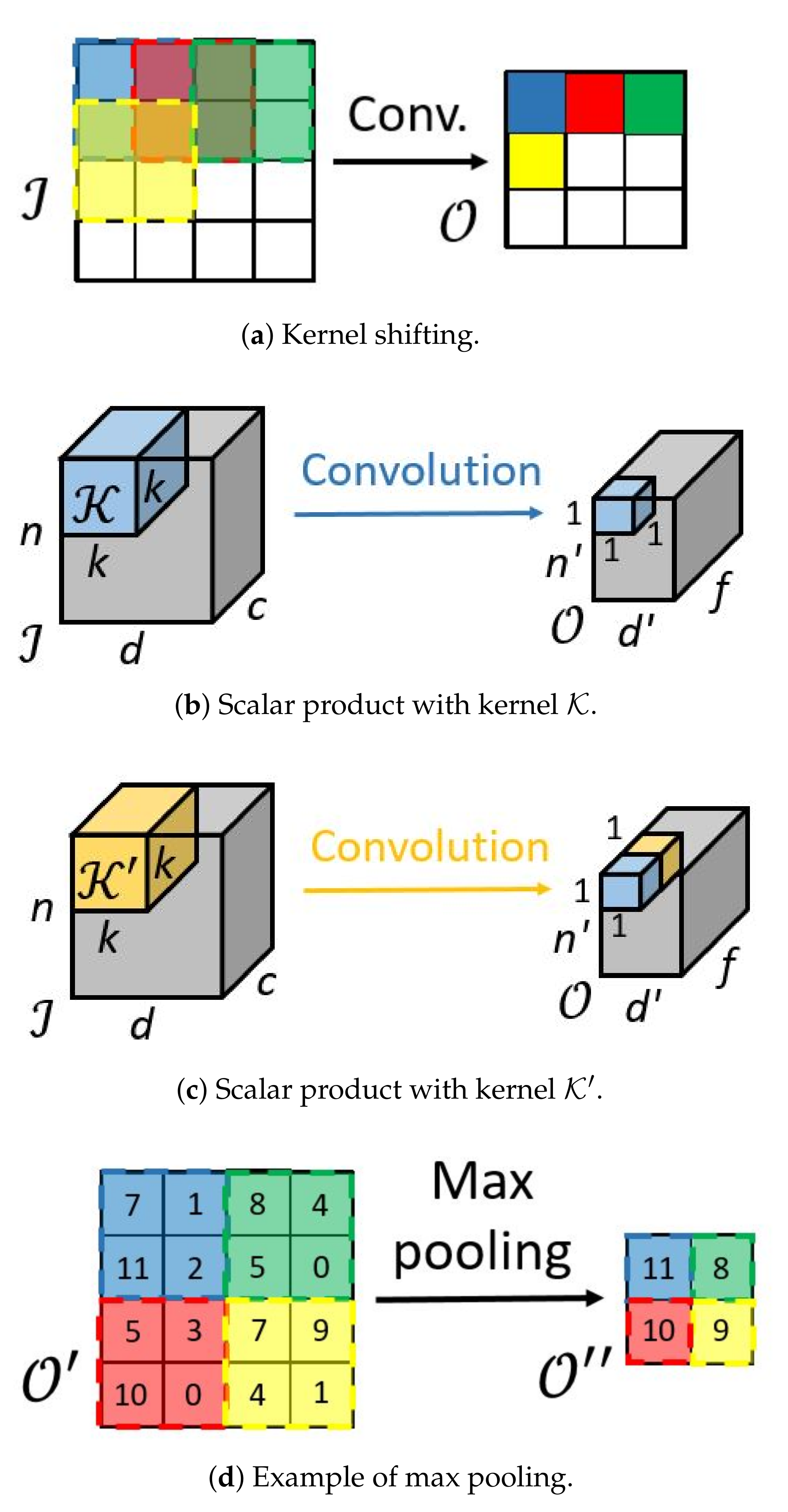
The present paper introduces a model for aging assessment based on CNNs, exploiting the ability of CNNs to deal with complex, non-linear problems when input data can be represented as tensors. A PD pattern represents partial discharges as a 2-dimensional array, that is, a second order tensor.
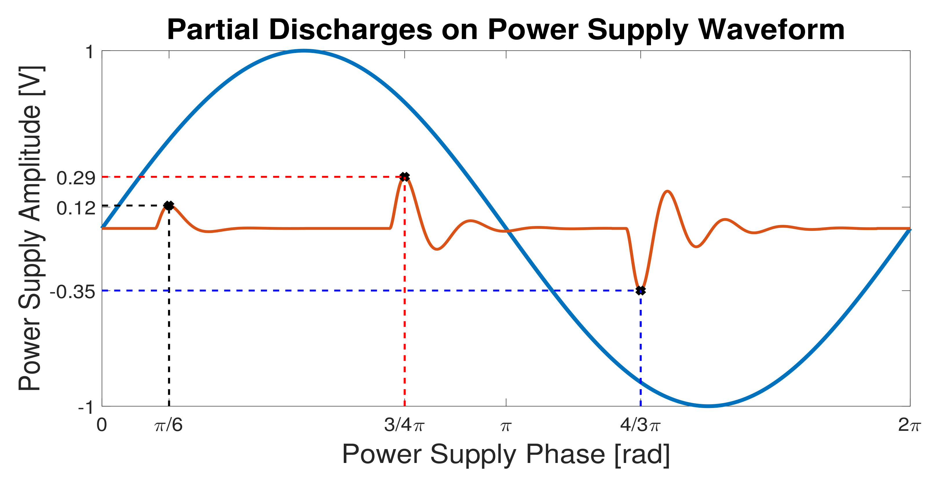
Figure 1 shows how the data collection mechanism is organized. In this plot, the blue line refers to the power supply voltage that sets the reference system for the apparatus under testing; the orange line refers to the partial discharges measured by a suitable sensor. In this example, three occurrences of PDs have been registered; each occurrence is characterized by a pair amplitude–phase. It is worth noting that this pair corresponds to the peak amplitude of a PD.
The corresponding PD pattern is organized as a matrix, the columns of which correspond to the power supply phases, and rows mark the maximum amplitudes of the discharges. Thus, each element in the matrix identifies an amplitude–phase pair; cell contents give the occurrences of discharges in a time window
.
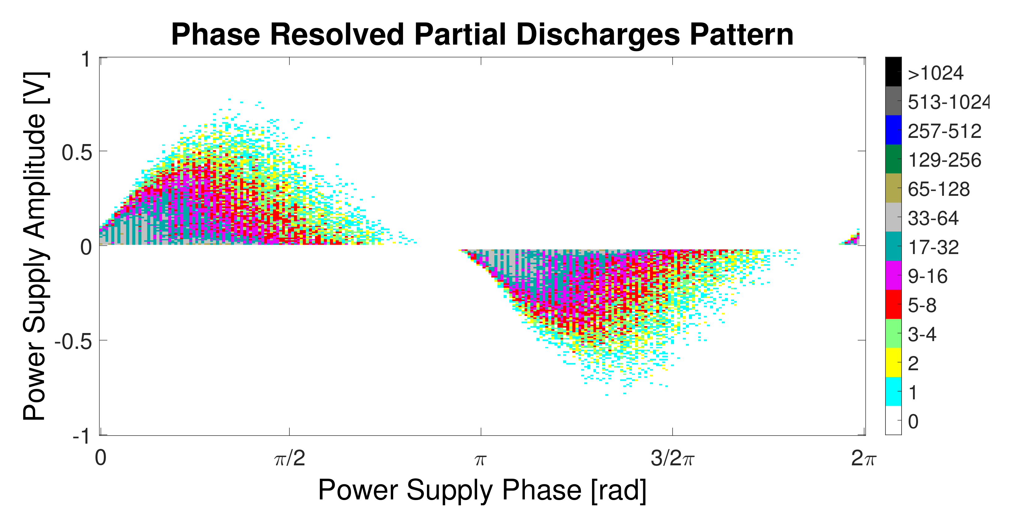
Figure 2 shows an example of a PD pattern.
Accordingly, PD patterns act as inputs for a 2-D CNN designed to infer the aging score of the monitored apparatus. Thus, the CNN supports a regression model that relies on the convolution operation. The regression model is trained by utilizing a proper dataset collected by monitoring a suitable number of apparatuses. Once trained, the model can assess the aging status of new, unseen apparatuses. The Appendix provides details about the general CNN architecture.
The first step in the design of the proposed framework is the definition of the aging score that characterizes the status of the monitored apparatus. The aging phenomena of electrical devices are expected to follow non-linear mechanisms. However, the output of the assessment framework should be analyzed by human users. Hence, a linear aging score seems more informative and easily understandable. Accordingly, an aging score of 0 is assigned to a specimen when the first PD phenomenon arises. An aging score of 0.5 characterizes a specimen at its half-life, while an aging score of 1 is reached when the breakdown is about to occur. This simple rule ensures that the network, when properly trained, will output a score that is user-friendly.
The collection of training data is another fundamental step. A dataset represents a specimen and it is collected from the inception of the first PD until the breakdown, capturing PD patterns at regular steps. Thus, a dataset is an ordered collection of PD patterns. The aging score assigned to the
ith PD pattern is:
where
is the starting acquisition time,
is the breakdown time, and
represents the acquisition time of
ith PD pattern in the dataset.
Eventually, the number of datasets matches the number of monitored specimens, and each dataset contains a variable number of PD patterns depending on the lifetime of the specimen, from the PD inception until the breakdown. The union of all the datasets makes the training set
, where
is a PD pattern and
the corresponding aging score. The cost function supporting the CNN training is the mean absolute error between the score inferred by the trained model,
, and the reference score
:
Thus, the loss function can be defined as the difference between the score inferred by the CNN and the score expected by assuming a linear behavior in the aging of the apparatus.
Summarizing the previous points, the proposed framework adopts a CNN to address a regression problem. At run-time, the CNN receives a PD pattern and infers the corresponding aging score of the monitored insulation system. To train this CNN, a set of specimens should be monitored until their breakdown to extract the PD patterns and the corresponding aging scores. These data make up the training set, that is, the ground truth supporting the learning process.
In addition, training involves model selection. In principle, the goal of model selection is to properly tune the parameters that characterize the CNN architecture; this process should lead to the final architecture of the CNN, that is, the architecture supporting aging assessment in the framework. On the one hand, the obvious target of model selection is to find the parameters setting that can lead to high accuracy in the prediction. Nonetheless, other constraints should be considered. As the number of layers grows, the number of parameters to be learned also grows. Moreover, the deeper the architecture, the larger the training set; in fact, one may face convergence problems in the training process if the size of the training set is not commensurate with the number of parameters to be learned. This aspect represents a crucial issue for the envisioned application because building a dataset is time consuming; as mentioned above, each specimen should be monitored from the PD inception until the breakdown. Hence, the admissible ranges for the parameters to be tuned should be set by also taking into account such constraints. In practice, one needs to balance the performance in terms of accuracy and the eventual complexity of the involved CNN.
Table 2 summarizes the quantities that were set via model selection, along with the admissible values:
The depth of the network, that is, the number of convolutional layers. The values ranged from 3 to 6;
The kernel size, which admitted two options: and ;
The number of neurons in the fully connected layer, which in the proposed framework involved a single hidden layer. The search space included three values: 16, 32 and 64.
The eventual architecture was also organized according to a few guidelines. First, each convolutional layer was followed by a non-linearity. Second, an average pooling was always stacked on top of two consecutive pairs (convolutional, non-linearity). Third, the number of kernels in the first convolutional layer was set to four. Indeed, starting from the second convolutional layer, the number of kernels always doubled. Doubling progressively the number of kernels is a common practice in deep learning; actually, each layer is designed to learn filters of increasing complexity. Accordingly, the level of abstraction of the features increases in the last layers of the CNNs. Thus, in an architecture with six convolutional layers one would see the following progression in the number of kernels: 4, 8, 16, 32, 64 and 128. Stride was always set to one.
4. Experimental Setup
The proposed framework has been tested on a specific scenario: the aging of twisted pair specimens. Low voltage stator windings of electrical machines are realized by means of wires insulated by enamels. Thus, the aging of twisted pair specimens can roughly simulate the turn-to-turn failures that can occur during the normal functioning of a winding motor. As a result, the development of predictive techniques for these specimens can be very useful to support the monitoring of low voltage motors insulated by enamels. Accordingly, all the twisted pair specimens involved in the present experimental session, insulated by conventional polyamide–imide enamel, were prepared according to the EIC 60851–5 standard. The following sections explain how training data were collected and how the training process was conducted.
4.1. Data Acquisition
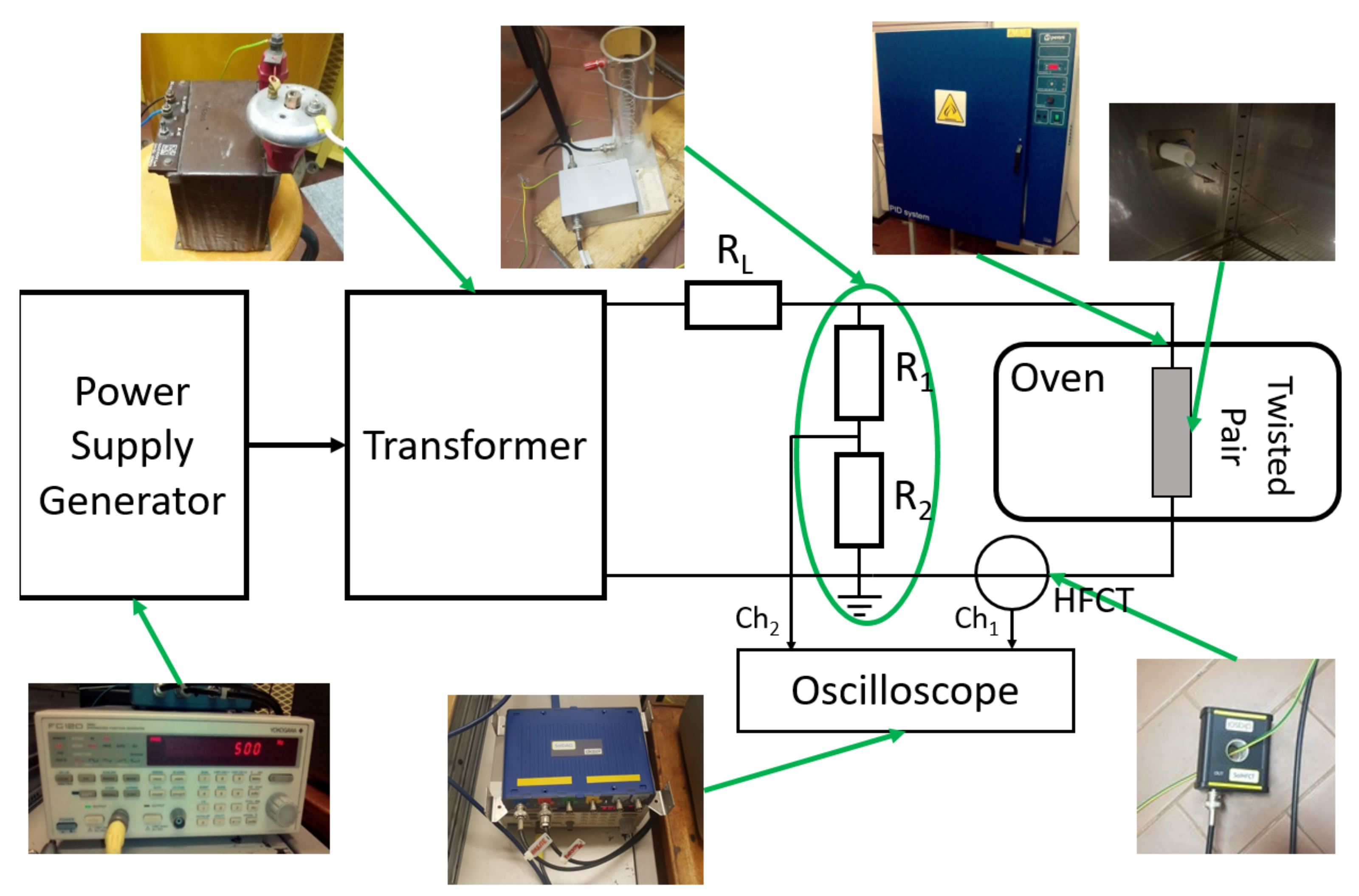
Figure 3 sketches the measurement system adopted to acquire data from a given specimen. A power supply generator provided a sinusoidal waveform with the frequency set to 500 Hz. PD signals affecting the specimen were measured via an HCFT sensor placed around the ground cable, with a band-pass behavior in the range [3 20] MHz. A Picoscope with a resolution of 8 bit, a maximum sampling frequency of 1 GSamples/s and a bandwidth of [0 200] MHz, sampled the PD signals and the power supply voltage. An oven sets the temperature to
, limiting the impact of environmental effects on the tests (i.e., humidity, non constant temperature, dust, etc.). For each specimen, the peak-to-peak voltage was kept constant. The experiment started at the inception of the first PD and ended at the breakdown of the specimen itself.
The experiments involved different settings for the voltage, as general aging phenomena depends on this parameter [
21,
27,
28,
29,
30]. In particular, aging is faster as the voltage increases. A total of 9 specimens were tested, with voltages ranging between 2000 V and 4000 V. In each experiment, the signals were sampled at regular steps
. The amplitude of the input voltage determined the value of
, which shortened as voltage increased.
Table 3 summarizes the acquisition features of the nine tests. The first column gives the supply voltage; for each row, the table provides the number of specimens tested, the number of PD patterns collected for each specimen, the value of
, and the acquisition time
utilized for extracting a PD pattern.
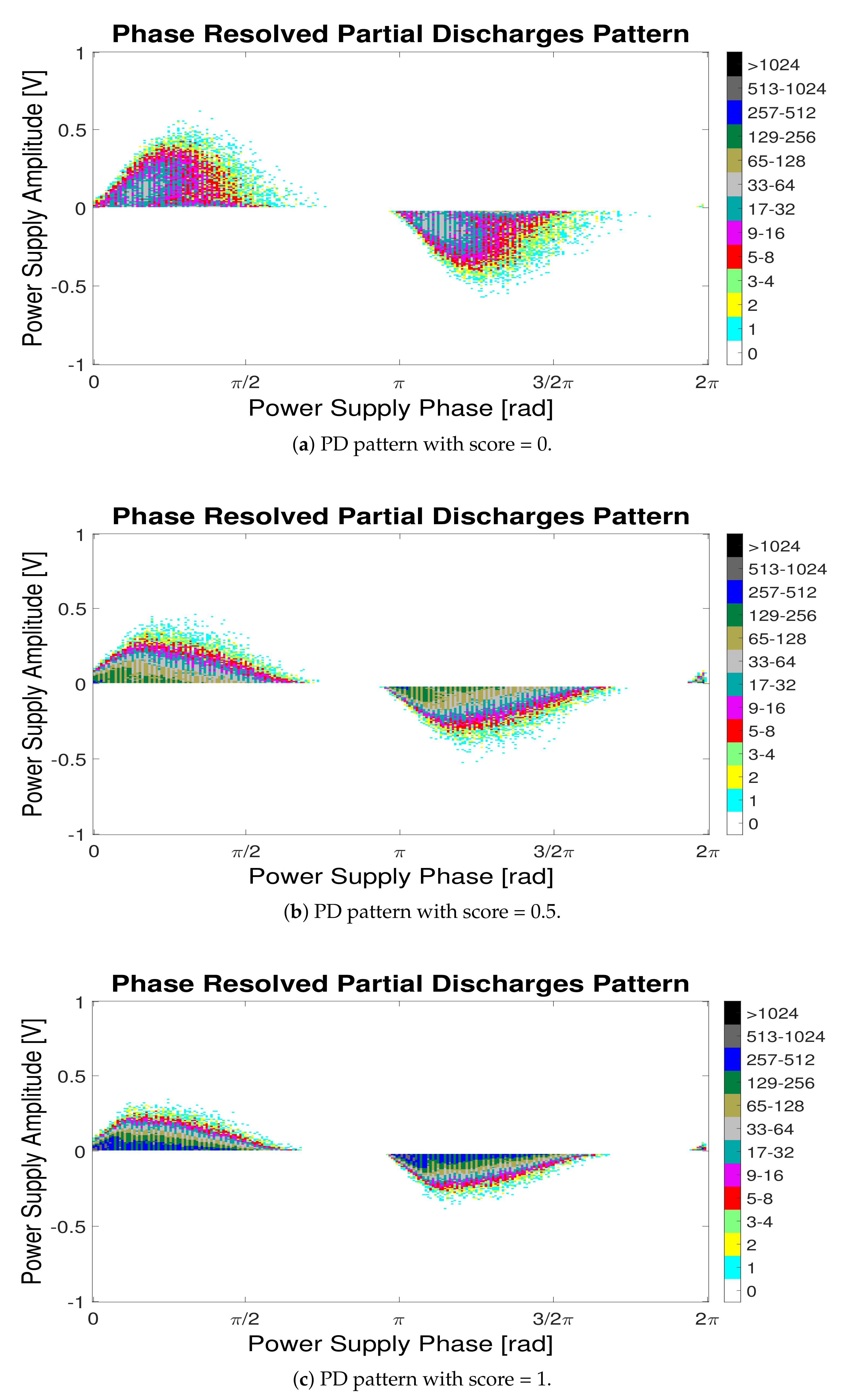
Figure 4 shows three PD patterns of a twisted pair specimen aged with a supply voltage of 2000 V. The PD patterns have been acquired in three different moments of the specimen lifespan: at the beginning of the PD activity (score = 0), at the half of the life (score = 0.5), and when the breakdown occurred (score = 1). During the aging of this kind of specimens, the partial discharges tend to increase their number, diminishing the amplitudes by taking into consideration the same acquisition time
. For each specimen, the whole PD pattern activity has been acquired from the beginning of the aging phenomenon until the disruptive discharge.
4.2. Training and Model Selection
The whole setup of the training and model selection took into consideration a major constraint: the limited availability of data acquired by monitoring the entire lifespan of a specimen. Such a process is usually expensive and time-consuming. Thus, it is reasonable to assume that one can only exploit a very small dataset. This constraint was indeed taken into account in the setup of the CNN architecture, as discussed in
Section 3. Actually, the present framework is designed to rely on a CNN characterized by a limited number of parameters just to avoid convergence issues in the training process.
In the present case, a total of nine specimens with as many experiments were available (as per
Table 3):
with
. The available dataset has been split into two non overlapping subsets, that is, a training set and a development set. The training set
included the data collected by seven out of the nine experiments. The development set
included the data collected by the remaining two experiments. This setup was adopted because consecutive PD patterns collected from the same specimen are expected to be strongly correlated.
Model selection was implemented according to the standard hold-out procedure. Thus, for each of the 24 admissible architectures resulting from the search space of
Table 2:
The architecture leading to the lowest mean absolute error was selected for the implementation of the eventual regression model. Algorithm 1 formalizes the steps.
| Algorithm 1 Model selection. |
Input Learning and selection for k = 1; k ; k++ do Train the k-th architecture with Test the k-th architecture with obtaining a loss score , according to ( 2) end for Output Return the best model configuration
|
5. Experimental Results
The experimental session aimed to evaluate the ability of the CNN-based model to infer the life status of a specimen. The implementation relied on Keras and Tensorflow.
Procedure 1 was adopted to set the configuration of the CNN architecture. The development set included data from one experiment at 2500 V and one experiment at 3500 V. The selected configuration corresponded to the following setup: 5 layers, kernel size = and 16 neurons in the fully connected layer.
The generalization performance of the model was evaluated by using a leave-one-out procedure. Thus, given the set
, six specimens out of seven were utilized in the learning process, while accuracy was assessed on the remaining specimen. This process was repeated seven times to cover all the possible configurations. Accordingly, in the following,
will refer to the vector of aging scores obtained when testing with specimen
j a CNN trained with the remaining six specimens.
is a vector as it collects the ordered sequence of predicted aging scores from
(first PD pattern extracted from the specimen under test) to
(last PD pattern extracted from the specimen under test). Algorithm 2 formalizes the evaluation process.
| Algorithm 2 Evaluation. |
Input Dataset Model configuration
Test the best model for
; ; do Train the model with , excluding the j-th specimen Test the trained model with the j-th specimen of Save the vector of aging scores in end for Output Return , with .
|
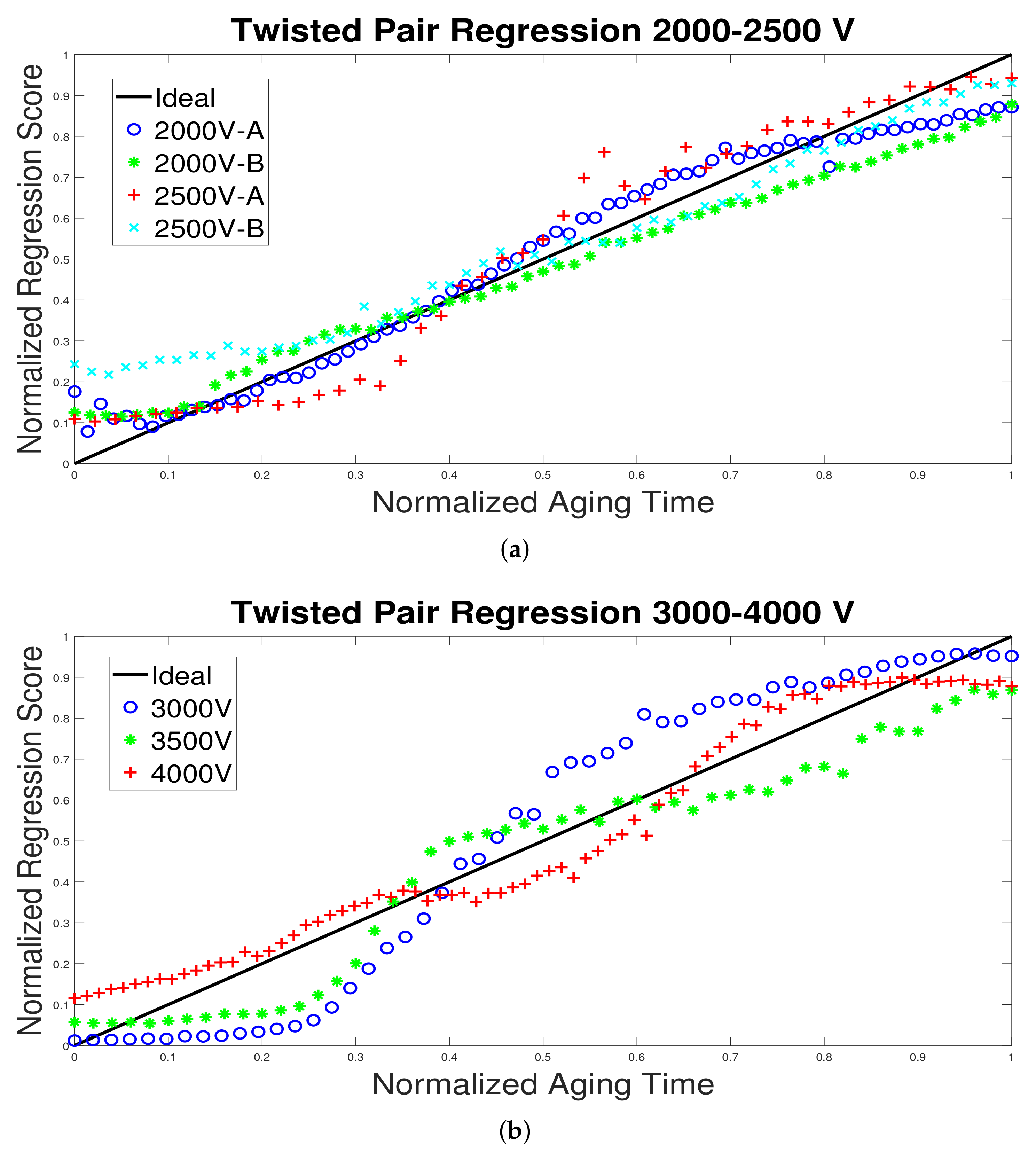
The outcomes of the seven experiments are grouped in two figures (
Figure 5a,b).
Figure 5a refers to the test involving the four specimens aged with a power supply voltage in the range
V. For each specimen, the figures show all the predicted scores
, that is, from the PD inception until the breakdown. It is worth stressing that during the online monitoring the CNN outputs only a score at a time, that is, when a PD pattern is collected. The figure shows the normalized aging time on the x-axis; that is, a value of 0.5 indicates that the specimen in that instant reached half of its lifetime. The y-axis shows the aging score inferred by the CNN after processing the PD pattern extracted at that instant: four different markers identify the outcomes of the four different experiments. The black line sets the ideal reference; in principle, at any instant the CNN should infer an aging score that corresponds to the normalized aging time. In general, the CNN proved able to estimate accurately the aging phenomena. Problems arise only in the very first part of the lifetime of the specimen. In fact, fast changes affect the insulation material when the PD inception occurs [
30,
31]. Hence, one may expect the model to be less accurate in that phase.
Figure 5b refers to the test involving the three specimens aged with a power supply voltage in the range
V. In this case, the level of accuracy reached by the CNN is lower. Actually, such an outcome confirms that aging phenomena significantly changes as voltage increases. Nevertheless, all the predictions show a similar trend, where the aging score increases almost monotonically. Thus, it is still possible to assess the aging status of the specimen. As, in practice, a predictive maintenance system aims to detect the insulation deterioration well before the breakdown, even a less accurate prediction can be useful.
6. Comparison with State-of-the-Art
This section compares the performance of the proposed CNN-based model with state-of-the-art approaches for aging assessment. The comparison involves (1) ML-based models and (2) explicit models that use empirical observation to set internal parameters.
The ML-based models rely on the approach utilized in designing the proposed framework: the features extracted from the PD pattern feed a regression model implemented by a standard machine learning paradigm. In this case, three different paradigms have been compared: multi-layer Neural Network (NN), linear Support Vector Machine (SVM), and kernel Support Vector Machine (K-SVM). The state-of-the-art provides works that proved the effectiveness of feature extraction techniques for PD pattern classification. In particular:
In [
42] the features are extracted using Local Binary Pattern (LBP) and Histogram of Oriented Gradient (HOG);
In [
43], the principal component analysis (PCA) of PD patterns sub-groups based on phase intervals is computed. Besides, the statistical moments (STAT) and the Weibull parameters (WB) from the PD pattern mean–pulse–height distribution and pulse–count distribution are extracted.
Such feature extraction methods can indeed support an aging assessment model. In addition, they proved effectiveness in other applications involving monitoring problems [
44,
45]. Actually, severity classification methods massively adopt PRPD statistical distributions and techniques based on the PCA to reduce the feature space [
14,
22,
23,
24].
The comparison with explicit models involved the approach presented in [
29,
30], which shares with the present work the experimental setup (i.e., only the voltage factor influenced the specimens under test, keeping the frequency and the temperature constant). In fact, several papers [
21,
27,
28] affirm that the most influencing factor on the aging condition is the power supply voltage. In the following,
Section 6.1 will present the outcomes of the experiments involving approaches based on the pair {feature extractor, ML}, while
Section 6.2 will present the outcomes of the experiments involving the model proposed in [
29,
30].
6.1. Comparison with Approaches Based on ML
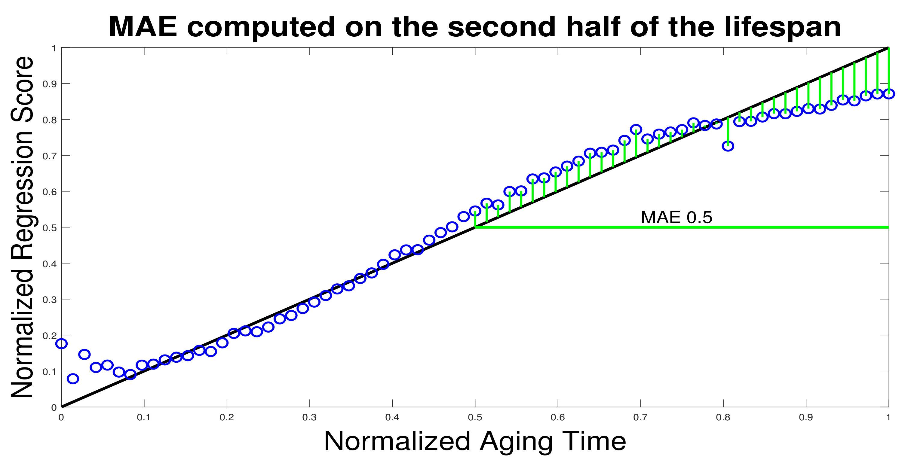
The performance of an aging assessment model can be characterized by measuring the absolute error between the predicted aging score at the instant i and the reference score set by the ideal behavior. In fact, one is interested in the distribution of the absolute error over a time window, since the goal is to evaluate the ability of the model to assess aging as the specimen progressively degrades. To the purpose of properly characterizing the performance of an aging assessment model in different conditions, the distribution of the absolute error over a given segment of the specimen lifetime was taken into account. Three segments were considered: the last 25% of the specimen lifespan, the last 50% of the specimen lifespan, and the entire specimen lifespan. Accordingly, the distribution of the absolute error over a given segment was characterized by computing the following quantities:
MAE: the mean absolute error over a segment
STD: the standard deviation of the absolute error over a segment
Here,
identifies the starting point of the segment taken into consideration. Thus, for example, to compute MAE and STD for the segment covering the last 50% of the specimen lifespan, one should set
. For the sake of clarity,
Figure 6 shows the corresponding configuration. The plot is structured as the plots in
Figure 5; thus, the x-axis gives the normalized aging time, while the y-axis gives the aging score inferred by the CNN after processing the PD pattern extracted at that instant. The blue markers identify the outcomes
of a predictor; the black line sets the ideal reference
. To compute the MAE for the segment involving the last 50% of the lifespan of a specimen, one relies only on the distribution of the absolute errors marked in green.
Table 4 reports the results of the experiments. The first column gives the feature extraction method. The second column identifies the segment of the lifespan utilized for computing MAE and STD. The third column presents the MAE scored by the best predictor over the three considered (NN, SVM, K-SVM). The fourth column displays the difference between the MAE reported in the third column and the corresponding MAE scored by the CNN-based model: a negative value means that the CNN-based model outperformed that predictor. The last column gives the ratio between the STD of the predictor and the STD obtained with the CNN-based model; a value larger than 1 means that the CNN-based model was characterized by a lower STD. Numerical outcomes show that, in general, the CNN-based framework always achieved better performances than the models based on predetermined feature spaces, both in terms of MAE and STD.
Figure 7 and
Figure 8 provide further details on the outcomes of these experiments.
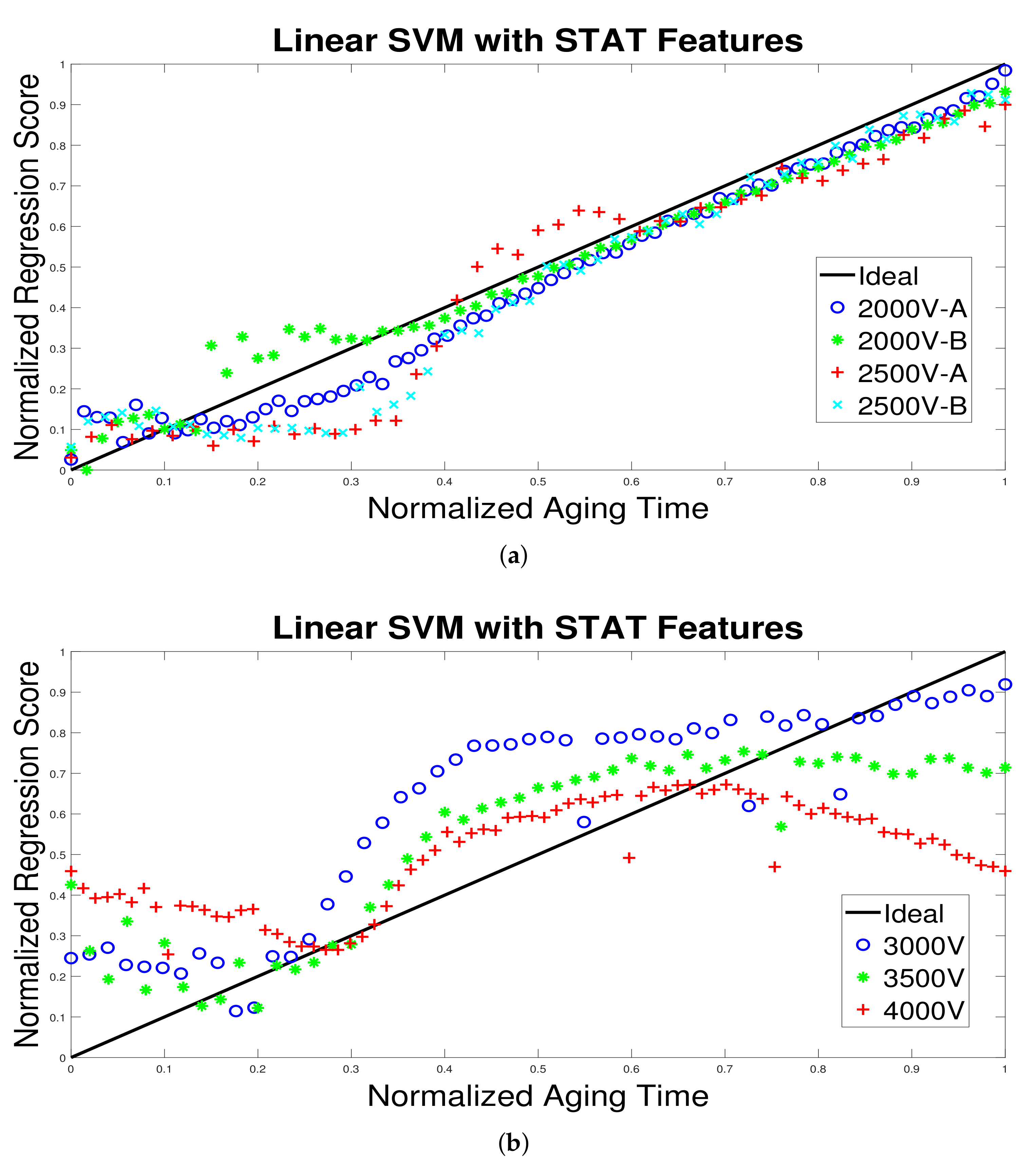
Figure 7 shows the results of the experiments involving a predictor based on linear SVM that processes STAT features; as per
Table 4, this predictor attained interesting performance in terms of MAE over the whole specimens lifespans. These plots are organized as the plots in
Figure 5, which showed the results of the experiments involving the CNN. Hence,
Figure 7a refers to the test involving the four specimens aged with a power supply voltage in the range
V, while
Figure 7b refers to the test involving the three specimens aged with a power supply voltage in the range
V.
Figure 7b proves that the predictor processing STAT features could not reliably predict the aging of the specimens under the configuration with a power supply voltage in the range
V. In particular, the unreliable predictions in the second half of the specimens life could be very dangerous, as the apparatus under monitoring is facing the risk of a sudden breakdown.
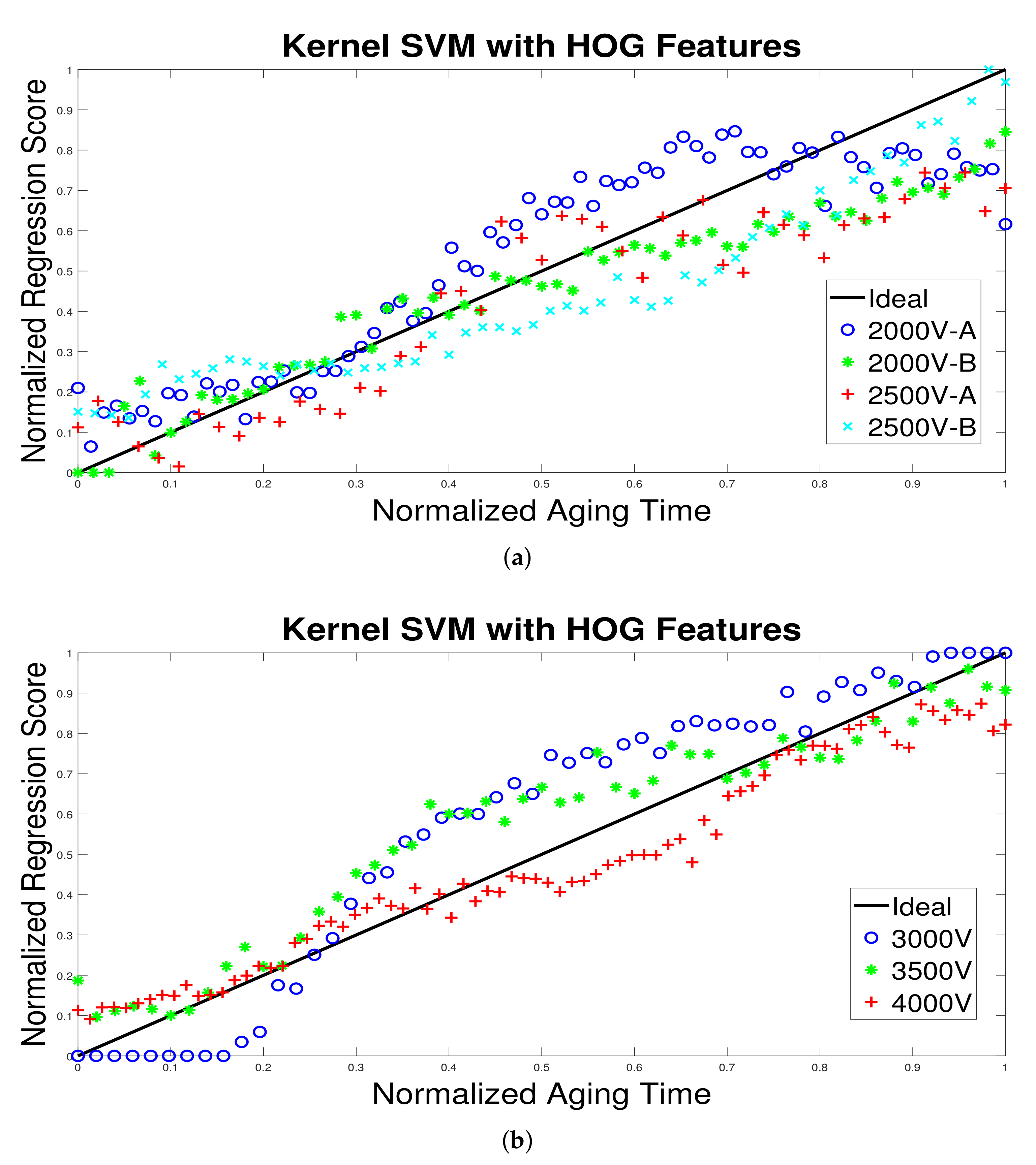
Figure 8 shows the results of the experiments involving a predictor based on kernel SVM that processes HOG features; as per
Table 4, such predictor also performed effectively in terms of MAE over the whole specimens lifespans. Again, the plots in
Figure 8 follow the same structure of the plots in
Figure 5. Both
Figure 8a,b show that this predictor lacked consistency over the different configurations of power supply voltage. In particular, three configurations proved critical:
,
, and
.
6.2. Comparison with the Explicit Empirical Model
The approach presented in [
29,
30] infers the breakdown time
D of an unseen specimen under the hypothesis that voltage is the only aging factor. It relies on two linear regression models. The first model is entitled to estimate the specimen parameters (
and
, Equation (
4) in [
29]); the second model computes the multi-linear regression coefficients characterizing the eventual prediction function (
K,
and
, Equation (6) in [
29]). Parameters
K,
and
are tuned by using a training set; however,
and
can be set only by monitoring the specimen itself for a certain amount of time.
According to the leave-one-out strategy (similarly to Procedure 2), six specimens out of the seven included in the training set were utilized to tune K, and . The remaining specimen played the role of the new, unseen apparatus. Thus, and were assessed by assuming that a given amount of time could be utilized only to monitor the specimen. In practice, given the specimen under test, D was obtained as follows:
Randomly set the starting point of the time window to be used to assess and ;
Set the length of the time window, collect data and compute and ;
Compute D.
The performance of the empirical model was again estimated by computing the absolute error between the predicted aging behavior (as per D) and the ideal behavior. Three different settings were adopted for the length of the time window: 10%, 25% and 50% of the specimen lifetime. Moreover, the MAE was averaged over 100 different runs, that is, 100 different random starting points.
Table 5 reports the outcomes of the experimental session. The organization of this table is similar to that of
Table 4. In the case of
Table 5, the first column refers to the length of the time window adopted in the experiments. The remaining columns give the same quantities of
Table 4 in the same order.
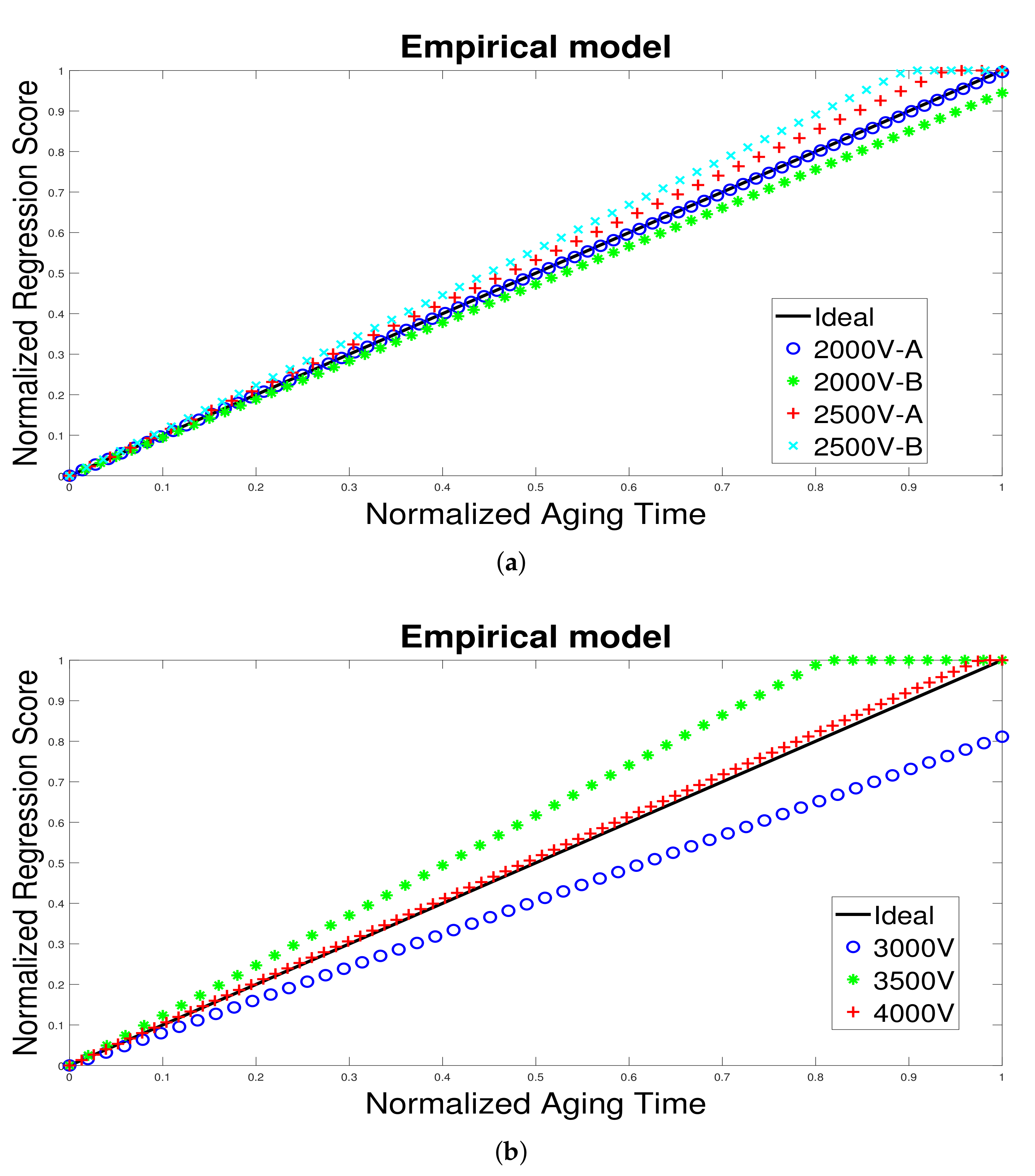
The table shows that the CNN-based framework was also able to outperform the empirical model. It is worth noting, though, that the empirical model attained its best performance when a longer time window was utilized to assess and , showing that this approach is not so effective for a real-time application. Such outcome emphasizes the advantages of the proposed architecture in giving a score with only one PD pattern.
Figure 9 shows the outcomes of the experiments involving the empirical model; as per
Table 5, the plots refer to the predictor that exploited 50% of time window to assess
and
, since that predictor scored the best MAE. The plots in
Figure 9 are structured as in
Figure 5. Hence,
Figure 9a refers to the test involving the four specimens aged with a power supply voltage in the range
V, while
Figure 9b refers to the test involving the three specimens aged with a power supply voltage in the range
V. As the empirical model relies on a prediction function built via linear regression, the seven predictors (four in
Figure 9a and three in
Figure 9b) only differ in the pair (
,
). The plots show that the empirical model failed to properly assess the aging process in particular with power supply voltages of 3000 V and 3500 V. In general, by adopting a linear model, one faces the risk of worsening the MAE in the last 25% of the specimen lifespan, which is actually the most critical segment.
7. Conclusions
This paper presented a novel strategy for the aging prediction of electrical insulation systems. Online aging monitoring is a crucial element for predictive maintenance. Indeed, the literature proves that this task is also very challenging. In several cases, aging prediction is approached as a severity technique, where the goal is to assign the monitored apparatus to a category that qualitatively characterizes the life conditions of the insulation system. The present research, conversely, introduced a framework that—in each instant—can assign an aging score to the insulation system.
The innovative content of the proposed method with respect to state-of-the-art approaches to aging monitoring lies in the ability of learning the feature set starting from a known dataset. In general, state-of-the-art approaches rely on the design of (1) hand-crafted features and (2) an explicit mathematical model that can properly map the feature set into aging scores. Both the tasks, though, involve time-consuming activities and require domain knowledge. In the proposed framework, the aging assessment model relies on PD patterns to obtain information about the partial discharge activity at a given instant. Then, a CNN architecture is demanded to complete feature extraction in the training process. Overall, one exploits the properties of CNNs to avoid issues such as (a) imposing strong assumptions on the relations between the life duration of the apparatus and factors such as power supply voltage, temperature, humidity, and so forth, and (b) modelling disruptive changes during aging.
The experimental activity focused on aging phenomena in twisted pair specimens, which actually can simulate the turn-to-turn failures that occur in winding motors. The CNN-based framework has been compared with two different state-of-the-art approaches:
ML-based model: ML is exploited to learn the mapping function between a set of hand-crafted features and the aging score;
Empirical model: the breakdown time of the apparatus is predicted via a multi-linear regression model.
In both cases, experimental outcomes showed the effectiveness of the CNN-based framework, which outperformed the other approaches. The most significant result is the ability of the CNN-based framework to attain consistent performances over different settings of the power supply voltage. This in turn confirmed that a CNN-based approach could better deal with the intricacies of the problem at-hand. The obtained results encourage the adoption of the same approach for more complex insulating systems with the aim of monitoring the related degradation by means of partial discharge measurements.


