Abstract
Hybridization of sources is spreading worldwide by utilizing renewable sources and storage units as standard parts of every grid. The conjunction of energy source and storage type open the door to reshaping the sustainability and robustness of the mains while improving system parameters such as efficiency and fuel consumption. The solution fits existing networks as well as new ones. The study proposes the creation of an accurate optimal sizing procedure for setting the required rating of each type of source. The first step is to model the storage and energy sources by using real experimental results for creating the generic database. Then, data on the mission profile, system constraints, and the minimization target function are inserted. The mission profile is then analyzed to determine the minimum and maximum energy source rating. Next, the real time energy management system controller is used to find the set of solutions for each available energy source and the optimal compatible storage in the revealed band to fulfil the mission task. A Pareto-curve is then plotted to present the optimal findings of the sizing procedure. Ultimately, the main research contribution is the far more accurate sizing results. A case study shows that relying on the standard method leads to noncompliance of sizing constraints, while the proposed procedure leads to fulfilling the mission successfully. First, by utilizing experimentally based energy and a storage unit. Second, by using the same real time energy management system controller in the sizing procedure.
1. Introduction
The reality of global warming and climate change caused by gas pollutants is no longer controversial [1]. However, the rise in energy demand has led to increased coal and oil production [2]. At the same time, governments across the world are encouraging the transition to renewable sources such as photo-voltaic (PV) [3], wind turbine (WT) [4,5], thermo-solar [6], fuel cell (FC) [7], hydropower [8], geothermal [9] and tidal & wave [10]. Some renewable sources (e.g., PV and WT) are stochastic and are not reliable. Moreover, from a grid stability point of view, when suppling energy from an electronic inverter and not from a synchronous machine, there is a lack of inertia and simple droop control is insufficient to stabilize the grid. Adding a grid-tied storage system solves the stochastic problem, and by adding a virtual inertia control loop [11] the stability issue is solved. The most common storage method worldwide is hydropower [12,13]. Today, the price of electrochemical storage is rapidly dropping, while the lithium-ion battery affords the highest energy density [14]. However, its lifetime and power density are limited. A super-capacitor contains the highest available power density and life cycle of 106 [15,16]. For improving the versatility of an energy storage system (ESS), it is common to connect both sources together in a single ESS [17,18]. When connecting two types of sources, there are some available topologies [14] of power converters [19]. Renewable sources with a varying maximum power point must be attached to a maximum power point controller [5] for increasing the harvested energy while integrating different types of sources is a common approach to benefit energy and power capabilities. Characterizing a source type can be easily done using a Ragone plot as presented in Figure 1. The chart presents a set of sources: as the source location is further to the right side, the source energy density is higher. As the source location is higher, then the power density is higher. For instance, FC is located on the far right and, therefore, contains very high energy density. However, the height of FC is low and, therefore, suffers from lack of power density. The outcome of this analyzation is that FC as a single source is sufficient to supply a very highly efficient energy source. Nonetheless, the FC is incapable of supporting an impulsive load. An alternative solution for long endurance load demand with a high-power burst is a combination of a high-energy source such as FC with a high-power density source such as a super-capacitor. The conjunction of source topology, whether it is passive or active, is set by the overall system requirement and the source operation range as elaborated in [14].
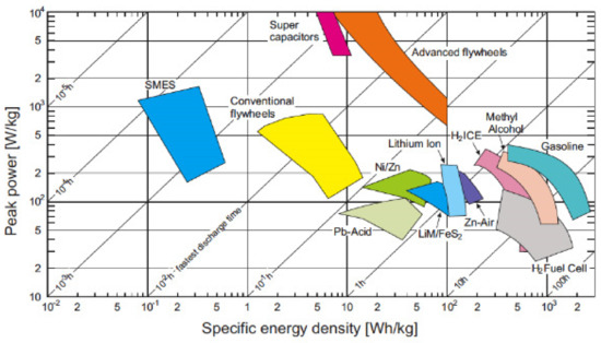
Figure 1.
Ragone chart [20].
The Tellegen theorem [21] forces a power equality of generating/sourcing on any operating grid. Until the late 20th century, the penetration rate of renewable sources was insignificant, and the grid stability was not dramatically affected by it. The constant increase of source mixture rate [22] along with stochastic energy production arose from the stability issue. Grid instability takes place when unfix frequency and/or voltage deviation occurs, therefore, nowadays an ESS is a mandatory element in any energy network. The big question that arises is how to determine the size of each source to face the load curve, as the size of any source decreases the device cost, fuel-consumption, maintenance, and operation prices. The design ambition is to set the minimum system according to the target minimization function. In systems where several requirements are applied, the weight of each one determines the overall target. The process for setting each source quantity is known as sizing [23,24,25,26]. The procedure’s methodologies [27,28] are well known and based on traditional methods such as the graphic construction method, iterative method, numerical method, probabilistic methods, and analytical method. More advanced methods are based on artificial intelligence such as genetic algorithms, particle swarm optimization, simulated annealing, ant colony optimization, artificial bee colonies, harmony searches, and cuckoo searches. Since any method/algorithm is imperfect, hybrid methods [29] are an effective combination of several different techniques, which utilize the positive influence of these techniques in obtaining optimal results for a specific design problem.
In a standard grid, the maximum load demand sets the rating of all summed possible available source loads plus system reserves. However, most of the points on the load curve are lower than the maximum power value. Therefore, some of the generation units operate far from the minimum fuel consumption point [30]. Moreover, the operation and maintenance cost increases in inefficient generation systems [30] along with the need to keep high-cost revolving reserves for an immediate response [31]. The analysis of a standard grid load curve in Figure 2 presents a decomposing of the power curve to an average power component and high-frequency harmonic components. The average load determines the minimum noncompulsory generator rated power where the ESS is at its highest rating. When selecting the minimum generation point (average power) together with a minimum required ESS, the source is obligated to engage in continuous operation, otherwise the load will fall. However, by increasing the ESS rating, the generation unit can operate at a minimum specific fuel consumption point with a start/stop mechanism. Hybridization of supply requires a real time control managing system for governing the operation of each unit and determines whether to run/idle the generators/sources and charge/discharge/idle the ESS. Stochastic sources complicate the management task. One of the approaches to stabilize the Tellegen equation is by transferring the stochastic source into the negative load [14], then all unknown parameters are summed into a single variable.
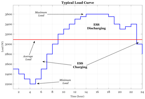
Figure 2.
Decomposing of typical load curve.
The sizing methods/algorithm is utilized for solving different kinds of problems; for instance, the hybrid vehicle energy system [32] and the hybridization of microgrids [33,34] and grids [35,36]. The sizing algorithm produces a set of minimal solutions that derive from the minimization target function known as the Pareto optimal curve [37]. Performing a sizing procedure for an energy system produces a two axis Pareto curve where the horizontal line presents an energy source’s nominal power rating and the perpendicular line represents the energy storage capacity in most cases, as presented in Figure 3. Every point in the sizing curve represents the minimum storage capacity required for a given generator rating. The curve divides the entire space into regions, a feasible and an infeasible region where the region above the curve represents the feasible region as any set of combinations for a generator power rating and battery capacity. The entire feasible region, including the sizing curve, is the design space for a given problem. It may be noted that the point where the sizing curve intersects with the horizontal axis represents the peak demand of the system where there is no need for an ESS and, therefore, the corresponding storage capacity is zero. On the other side, the curve ends at the average required power that reflects the minimum size of the generator, which guarantees to finish the power profile with the same state of charge (SoC) at the ESS. In a non-repetitive power system, the ESS could fulfill the load mission without any long endurance energy source (e.g., diesel generator). At the end of the process, the ESS is empty/near empty and cannot support another cycle. However, when performing a sizing procedure for a sustainable grid, the minimum generator size is mandatory.
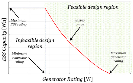
Figure 3.
Typical sizing Pareto curve.
Although the sizing procedure is a well-known technique, its results are insufficient and inaccurate since researchers [33,34,35,36] use the rated power of sources and rated capacity of ESS. However, the real power and efficiency of any source are a function of the operating point and include internal parasitic elements that affect their performance. For instance, when using the gross ESS data of capacity, the actual amount of energy is much lower. According to the manufacturer’s datasheet [38], the rated capacitance is stated at discharging of 0.2C-rate, while at 1C-rate the cell will lose all energy within less than one hour. Therefore, the planned task will go unfulfilled. Moreover, in standard sizing procedures, sources such as internal-combustion generators are utilized as a nominal rated source. However, the generator operating point sets the generator output impedance, which has a great impact on generator efficiency as well as on other operating sources on the same grid. Since the present sizing procedure is inexact and increases the probability to failure in fulfilling the mission task, a revised procedure is required. The objectives of this research are to create a generic tool for sizing and operating hybrid energy sources based on a statistical load profile while respecting a set of certain optimization constraints. This study will demonstrate an optimal mix of electrical sources while enabling a fuel-consumption minimizing energy management strategy. In contrast to the majority of methods aiming to tackle a similar problem, here the expected contribution is two-fold: (a) a realistic instantaneous performance of each source will be utilized in the design and (b) a sizing process exhibits an energy management strategy expected to be executed during real-time hybrid energy source exploitation. The former will be accomplished by investigating characteristics of the representative line of batteries and generators in order to link figures of merit provided in the datasheet to instantaneous performance of these devices under various operating conditions and derive the generic performance of each source. The most important characteristics are charge/discharge curves for different temperatures and discharge rates, allowing for the performance estimation for a wide range of operating conditions at various life cycle stages.
In this paper, a new method for a sizing procedure based on actual performance of modeled energy units is presented. First, a generic model for an ESS and for a high endurance energy source (diesel generator) is presented. Then, a sizing procedure is performed based on the proposed models and the results are verified in a system level simulation. Thus, experimental results are generated to validate the proposed theory versus the conventional one.
2. Energy Unit Modeling
By transferring the sources to a digital model, examination of possible lists of solutions for the sizing procedure is expedited. The first step is creating a trustworthy model of each simulated source. Researchers have developed several approaches for energy source modeling. Each method brings different levels of accuracy and complexity with pros and cons. These models can be generally divided into three groups: the electrochemical [39]/electromechanical [40] model, the equivalent electric circuit models [41,42], and the mathematical model (analytical or stochastic) [43,44]. Theoretical models that are solely based on manufacturer data are insufficient to accurately imitate an actual operation of any energy source at all operating points [16]. To improve model accuracy, a new combination of methods of the dominant electric models along with interpolation and extrapolation approximation are herein applied. The method utilizes actual energy unit performance with probabilistic analyzation and an equivalent electrical circuit.
2.1. ESS Modeling
The first step for ESS modeling for creating a generic ESS model is the algorithm procedure. The models that are founded on electrochemical equations or equivalent electrical circuits are inherently inaccurate within a production series. Thus, a lookup table based on average experimental results is more efficient in prognosticating ESS parameters and behavior. The high-level ESS model algorithm includes the following steps: It begins in block 1 (Figure 4), the model receives the load power demand and in the case of external sources the produced power by the source. This is shown by using the power balancing Equation (1) determining the ESS status for charging or discharging. Where is the discrete actual power value of ESS (supplied or accumulated), is the discrete present load power demand, and is the discrete generator power.
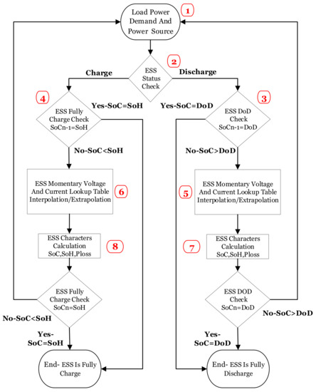
Figure 4.
Generic ESS model algorithm.
Then, the model processes the absolute value of power and divides it by the ESS presented internal voltage value () and verifies that the model operates within the allowed ESS current. With each cycle/start of operation, the SoC and depth of discharge (DoD) values can be modified to a specific value, otherwise the model inherits their values from the previous stage (n − 1). The ESS model can also receive any desired ambient temperature (within the allowed boundaries) or a varying temperature profile or a constant. In block 2, the model translates the power demand into an instruction for charging or discharging. The model inspects the instantaneous current by sensing the ESS internal voltage. Before starting a charge or discharge procedure, the model examines the following conditions (2a,b) in blocks 3, 4.
where is the discrete previous SoC value, is the ESS nominal capacity, is the minimal capacity, and is the discrete previous DoD value. The calculated ESS current () and internal voltage () are then processed in blocks 5, 6 (discharging and charging, respectively). The model shows the following parameters: instantaneous terminal voltage, battery power, energy, capacity, wasted power and energy, the remaining energy, and the updated capacity. If the ESS is fully loaded, the process ends. Otherwise, the linear interpolation/extrapolation begins in block 6. The charging process ends where the algorithm calculates the updates for the ESS parameters in block 8 and starts the next cycle. The second option is the discharge path: the model verifies that the status of the ESS is not beyond the DoD boundaries in block 3. If the ESS is fully discharged, the process ends. Otherwise, the linear interpolation/extrapolation begins in block 5. The discharging process ends where the algorithm calculates the updates for the ESS parameters in block 7 and starts the next cycle.
The internal voltage and ESS current are now processed and supply data on the momentary ESS capacity, ESS supply energy, energy loss, and energy remaining. The forward Euler method is a first-order method, which means that the error per step is proportional to the square of the step size, and the error at a given time (global error) is proportional to the step size. The momentary ESS capacity is estimated by the discrete forward Euler method [45] as presented in (3). The ESS current is accumulated and adds/subtracts from the present capacity in charge/discharge mode, respectively.
where is the discrete momentary capacity value, is the previous discrete momentary capacity value, is the ESS constant, and are the previous and actual time steps, and is the discrete previous ESS supplied current value. The ESS supplied/sourced (momentary) energy is also estimated by the forward Euler method. The ESS internal voltage is multiplied by the ESS current resulting in ESS power that has accumulated into ESS energy, as presented in (4). Where is the discrete internal momentary ESS energy, is the previous discrete internal momentary ESS energy value, is the ESS constant, and are the previous and actual time steps, is the discrete previous ESS external voltage value, and is the discrete previous ESS supplied current value.
The ESS energy loss is similarly defined by the forward Euler method. The ESS current is squared and multiplied by the interpolated ESS internal resistance resulting in ESS energy loss as presented in (5).
where is the ESS internal energy losses, is the previous ESS internal energy losses, is the ESS constant, and are the previous and actual time steps, is the discrete previous ESS supplied current value, and is the ESS internal resistance. Now, the remaining stored energy is revealed in (6):
where is the ESS energy, is the initial ESS energy, is the discrete internal momentary ESS energy, and is the ESS internal energy losses. The model receives the mentioned parameters and produces the ESS terminal voltage by the linear-point slope algorithm (). The approximation procedure output is the ESS terminal voltage. With the use of approximation of the internal resistance (), the internal ESS is revealed. The ESS internal voltage () is the keystone for showing the above parameters and, therefore, the heart of this model. The approximation of the ESS internal resistance is also based on the linear-point slope algorithm. The database contains rows, columns, and pages of measured values on impedance, current, temperature, and calculated SoC. The approximation procedure collects data on three mentioned parameters and supplies the present value of the ESS internal resistance (). The ESS SoC calculation is made by the discrete forward Euler method for the momentary capacity (3) and the initial capacity summation. In this method, the actual capacity value is set as the ESS SoC, with another option to present the SoC in percentage as shown in (7a,b). Where is the SoC value that is equal to the ESS actual capacity, the , is the initial ESS capacity, is the discrete momentary capacity value, is the SoC value in percentage, and is the ESS nominal capacity.
2.2. Generator Modeling
Generator modeling is a very complicated and non-trivial task; the model is constructed by two key elements: a synchronous generator (SG) and a diesel engine. As for the ESS, the generator model also utilized fuel consumption from experimental results into lookup table. Then, the actual fuel consumption is estimated by the discrete forward Euler method [45]. The SG model comprises a mechanical and an electrical part: the mechanical side receives the torque and the mechanical power. Then, analyzation is carried out exhibiting the electric power, electrical torque, electrical frequency, and the grid angle theta (). These parameters are processed in the electrical part by performing a park transformation [46] that expresses three-phase voltages and current in terms of the orthogonal basis in (). The results of the park transformation define the synchronous machine equations for the stator voltage and as
where and are the d-axis and q-axis voltages behind the subtransient reactances, and are the d-axis and q-axis currents, and and are the d-axis and q-axis subtransient reactances. The model requires data about SG rating (nominal voltage, current and frequency) and also parameters such as the synchronous reactances , the transient reactance , , the d-axis and q-axis subtransient open-circuit time constants and , and the d-axis transient open-circuit time constant . The SG model supplies the set of parameters: for instance, the mechanical rotor speed , stator terminal voltage , , and stator line current , . The rotor speed is fed into the diesel engine governor. Then, by referring it to the synchronous velocity and performing an analysis of the new engine, mechanical torque is revealed and, therefore, the required mechanical power for driving the SG. The SG line power is revealed by processing the mentioned stator voltages and currents. Using the forward Euler method, the fuel diesel engine consumption is:
where is the hourly fuel consumption, is the SG source power, and are parameters of the SG source power curve. The generator model algorithm is presented in Figure 5. The model receives the mechanical velocity () and the reference , then analyzes the error, adjusts the diesel engine velocity, and supplies the mechanical power to the SG. The SG produces line voltages and currents, then the excitation controller adjusts the field current to balance the power demand. By using the generator measurements, the generator’s electrical power is calculated, and the data is formulated with a linear point-slope method (interpolation and extrapolation). Based on the generator experimental results, the fuel consumption is then estimated.
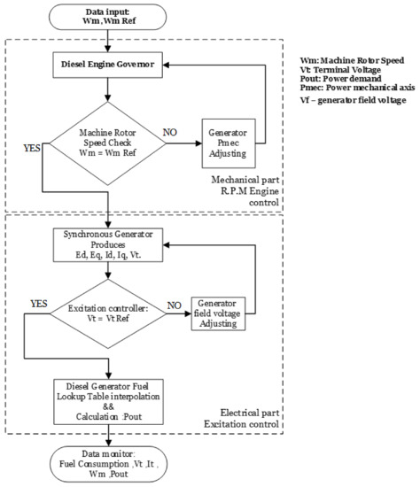
Figure 5.
Generic ESS model algorithm.
3. Sizing Procedure
For performing proper hybrid energy source sizing, the load profile is defined first. In contrast to most previous works [24,25,26,27], we will consider a statistical rather than analytical load profile to approach as close as possible a realistic situation. The minimization target function is defined next for one or more variables as minimum fuel, maintenance cost, operating cost, initial cost, volume, weight, etc. Then, the system constraints such as load voltage range, generator power, variation rate, or ESS charge/discharge rate, etc. are determined to prevent unrealistic solutions proposed by sizing procedures. The real device’s database is also presented to allow for inclusion of existing devices into the hybrid source and connecting these via realistic power converters. The sizing procedure is decoupled from the load profile into static and dynamic components. The energy source is utilized as the supply source of the static component while the power source requires the absorbing and releasing of the dynamic component. Every power system is governed by a real time energy management controller that behaves in a specific manner according to its design rules. A sizing algorithm from previous works [24,25,26,27] does not utilize the real time system management controller in the analysis procedures. Since the real time controller dramatically affects the operation of each source, it must take place as a system manager in the sizing procedure as well. The proposed sizing is presented in Figure 6 and operates as follows: The first step is establishing a database with units of energy sources and storage units as elaborated in the second paragraph. Then, a statistical power curve is applied as the referenced load profile. In contrast to traditional sizing approaches, the procedure is centered on a statistical rather than analytical load profile as close as possible to a realistic situation. The constraints are introduced preventing unrealistic solutions proposed by the sizing algorithm. The minimization target function is added into the algorithm with a specific weight for each target. The algorithm calls the modeled real devices from the introduced database. Gathering all system information and requirements leads to the data processing stage where the algorithm verifies all acceptable source solutions with the specific selected path for solution by running the system real time energy management algorithm. The energy management strategy is a real-time high-level supervising routine aimed at commanding the instantaneous operating power of each hybrid source component. Referring to a general fully controlled energy-storage source system, the energy management strategy calculates reference power commands for each component based on instantaneous load demand, operating mode, and feedback from each component, considering each component’s constraints in both time and frequency domains. The controller, executing the energy management strategy, must determine the amount of power instantaneously drawn from each component to minimize the target function (e.g., fuel consumption). To accomplish this, the procedure requires as much available data as possible such as a consumption map of the energy/storage source that is accurately determined for all the expected operating points and is included in the sizing database.
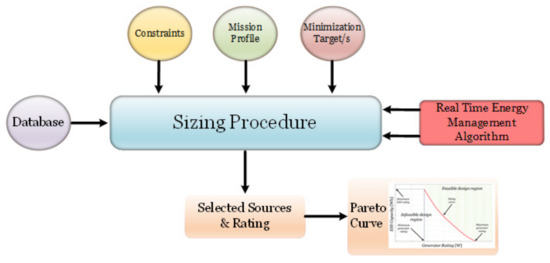
Figure 6.
Sizing process.
The proposed sizing methodology offers two types of sources, power, and energy. The analyzation of power curves reveals the average power and maximum required power. For sustainable and reliable energy supply, the energy source’s minimum rating is the average power, otherwise the cyclic mission criterion will not be completed. The minimum energy source (MES) is, therefore, set at the lower boundary for the sum of all energy sources. On the other hand, the peak power demand sets the upper boundary for the total energy source rating. Thus, the feasible solutions for utilization of energy source (ES) exist in this band as formulated in (10).
The rating of an energy storage is derived from the size of the energy source. The minimum energy storage (MEST) source is set at the maximum power demand and, therefore, the maximum size of storage at the minimum energy source. Performing the analysis on real modeled sources governed by a real time energy management system controller (EMSC) reveals the optimal fitness solution for all available rated energy sources specific to the MES point. Thus, the possible solutions for employing an energy storage system (ESS) source with a specific energy source exist in these borders as explicated in (11).
The proposed sizing algorithm presented in Figure 7 operates as follows: the operator inserts information regarding the mission profiles (e.g., power), the required constraints (e.g., DoD), and the minimization target functions (e.g., fuel). Then, the subprocess of sizing analyzation takes place where the search is based on existing modeled sources from the sizing database, beginning at the MES point and evaluating the optimal solution route managed by the EMSC for fulfilling the mission criterion. Then, the procedure continuously increases the energy source value for the next available modeled energy source. The cyclic calculating fitness for optimal sizing ends at the point where the routine incremental energy source reaches the maximum power demand value of the mission profile where the energy storage unit is useless. Then, the algorithm collects all minimal sets of solutions and plots the Pareto-curve as an aggregation of optimal energy storage units with energy source units (e.g., Figure 3).
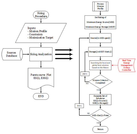
Figure 7.
Generic sizing algorithm.
4. Design Example
To validate the proposed theory, a case study was conducted. A synchronous fuel-based generator was utilized as an energy source and a lithium iron phosphate (LiFePO4) battery was employed as an energy storage system. First, the family of sources were modeled based on experimental results at different currents and power rates while varying the environmental temperature. The basic cell parameters are presented in Table 1. The ANR26650M1-B of the A123 cell was tested under different power and current levels for charging and discharging at different temperatures. The experimental results were assembled into a collected database as a base for predicting the battery’s exact terminal voltage and current.

Table 1.
The ANR26650M1-B of A123 cell parameters.
The battery model was designed using a MATLAB-SIMULINK simulation tool. The model receives the load power demand and the generator supply power, and using Equations (1)–(7) it produces the following parameters: the requested battery power, produced battery power, battery power, battery terminal voltage, battery internal voltage, battery capacity, battery instantaneous power, battery SoC, battery state of health (SoH) and battery power dissipation. All parameters are presented in the operator workspace and are available for use for sizing simulation tools. Since most loads source a specific power, when the battery voltage starts to drop, the battery current rises. Verification of the model’s behavior was made under a constant power demand and equates with the experimental results and other available models for charging at a constant power of 16.6 W and discharging for 16.6 W, as presented in Figure 8 and Figure 9. The model predicts the battery’s behavior very accurately and offers excellent performance as a reliable simulation tool for the sizing algorithm. The generator family was based on a family of HATZ diesel engines driving a three-phase generator () while using Equations (8) and (9). Then, a load power profile (Figure 10) was loaded into the sizing procedure that showed the load average power.
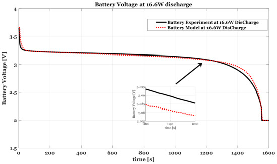
Figure 8.
Battery model versus experimental results: Battery discharge voltage at 16.6 W (black–experimental, and red–simulation).
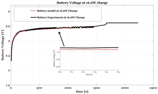
Figure 9.
Battery model versus experimental results: Battery charge voltage at 16.6 W (black–experimental, and red–simulation).
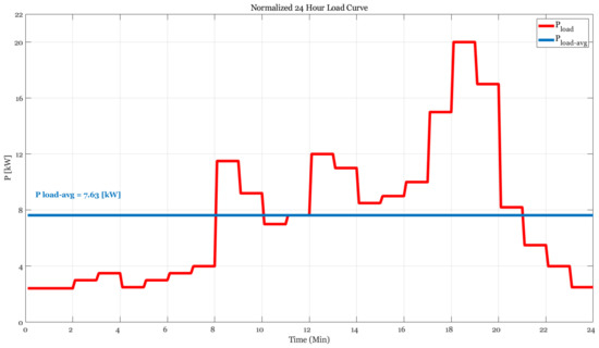
Figure 10.
Normalized load power profile.
The algorithm then allocates from the database the available suitable generator with a nominal operating power equal or near equal to the average load power 7.6 kW. Next, the algorithm searches for an optimal storage system to fulfil the required load curve based on the real time system EMSC. In the next step, the following (increase) available generator model in the database is utilized as the energy source. Again, the algorithm searches for optimal storage by using EMSC. The procedure continues until the energy source is equal to the maximum power load and a Pareto curve is then generated. The sizing result of the proposed new procedure is presented (red) in Figure 10 versus the conventional approach (blue). The traditional procedure results are a set of a particular generator along with the required ESS; however, in the new procedure, for a specific rated generator, the ESS is slightly higher than what is habitual. These results are reasonable since every device contains parasitic elements that create internal losses, requiring the increase of ESS to compensate for the missing energy. Since the load average power is 7.6 kW, the minimum generator rating is equal to this value. The peak load power is 20 kW, therefore, this is the value of the maximum rated generator. To validate the findings, a case study was conducted. By selecting a scenario of continuous generator operation with a constraint of minimum fuel consumption a selection of two sets of points is presented. A 9.6 kW generator point is selected and two ESS revealed from the Pareto curve are presented in Figure 11 (red). To validate the proposed theory, a standard sizing procedure was conducted, with the results presented in Figure 11 (blue).
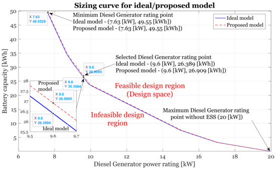
Figure 11.
Pareto curve results.
Based on the sizing results, the initial point of optimal fuel consumption was selected as well as the complementary storage unit, as shown in Figure 11. The setup includes a 12.6 kVA generator utilized as the energy source, a three phase Vienna rectifier, a three level DC bus (+400 V, 0 V, −400 V), two bi-directional isolated H-Bridge ZVS converters connecting the 23 Ah, LiFePO4 battery storage system to the DC bus, and a neutral clamp point three phase inverter that feeds the load. The system signals were captured by a four channel Rohde & Schwarz RTM3004 digital oscilloscope equipped with differential voltage probes and AC+DC current probes. Moreover, a Fluke n-daq data logger collected all required system data (voltages, currents and temperatures), as presented in Figure 12.
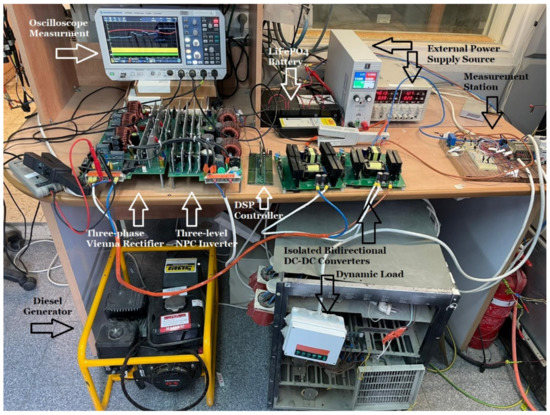
Figure 12.
System setup.
The experimental results of the sizing procedure based on real unit modeling show that the generator power is constant at the minimum fuel consumption point across the entire load curve. When the generated power is higher than the load demands, the energy storage unit absorbs the surplus power. In the case of lack of power generation, the ESS supplies the missing amount of power, as presented in Figure 13a,b. Battery SoC at the end of the load cycle is the same as at the beginning (Figure 14), therefore, the system can continuously run while keeping the load operation.
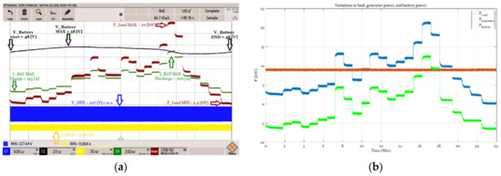
Figure 13.
Experimental results based on the new sizing procedure: (a) system voltage currents and power on oscilloscope. (b) MATLAB processed power system balancing (blue–load, green–battery, and red–generator).
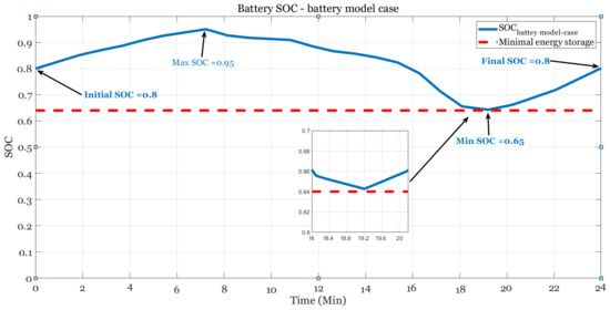
Figure 14.
Battery SoC during the load cycle based on the new sizing procedure.
However, when performing standard sizing based on manufacturer data while going through the load profile with a different EMSC, the sizing results show that the ESS has reached its minimum SoC point with the DoD attaining the lowest level. To avoid load shedding the EMSC increases the generator power (Figure 15b—circled in red) to compensate for the missing requirement power, EMSC also allow the ESS to get under the DoD. When the load demand is dropped, the EMSC returns to the minimum fuel consumption mode and recharges the ESS, as presented in Figure 15a,b and Figure 16.
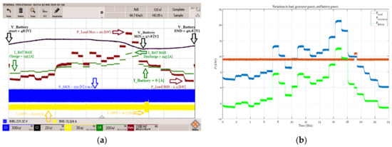
Figure 15.
Experimental results based on standard sizing procedure: (a) system voltage currents and power on oscilloscope. (b) MATLAB processed power system balancing (blue–load, green–battery, and red–generator).
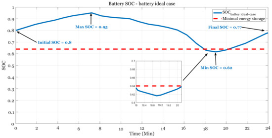
Figure 16.
Battery SoC during the load cycle based on standard sizing procedure.
5. Conclusions
A new sizing method was presented in this paper. The proposed procedure was examined with a case study of normalized residential load profile. A hybrid generator with a storage system was modeled and utilized as the sizing database source. Based on sizing algorithm results, a Pareto curve was plotted, presenting the optimal set of solutions for each source together with results of the standard sizing method. It was shown that the new procedure that includes unit modeling based on experimental results and an algorithm that utilized the original EMSC within the sizing procedure supplies accurate results with respect to the standard method. The real system experiment shows that the new procedure enables minimum fuel consumption while operating inside the SoC boundaries and finishes the load cycle at the same point of SoC as the initial value. Additionally, in the case of using a standard known sizing procedure that does not consider the real behavior of sources, the hybrid system cannot finish the load cycle while keeping the generator minimum fuel consumption point, as well as the initial ESS SoC. The proposed solution is optimal only for the specific load profile, target function, and system constraints. Presuming an additional target function of minimum volume with the same load profile could lead to a higher rating generator and smaller ESS. On the other hand, the same case with a modified DoD constraint equal to 0.5 would decrease the ESS capacity while keeping the generator at the same operating point. Moreover, additional sources such as PV, WT, super-capacitor, etc. that are not included in this research would have a major influence on sizing results and are left for future research.
Author Contributions
Conceptualization, I.A. and N.A.; methodology, I.A. and A.S.; software, I.A., M.C., N.A., and A.S.; validation, M.C., N.A., and A.S.; formal analysis, I.A. and N.A.; investigation, I.A. and N.A.; resources, N.A. and A.S.; data curation, I.A. and A.S.; writing—original draft preparation, I.A. and N.A.; writing—review and editing, I.A. and A.S.; visualization, I.A.; supervision, I.A.; project administration, I.A. All authors have read and agreed to the published version of the manuscript.
Funding
This research received no external funding.
Institutional Review Board Statement
Not applicable.
Informed Consent Statement
Not applicable.
Data Availability Statement
Not applicable.
Conflicts of Interest
The authors declare no conflict of interest.
Abbreviations
The following abbreviations and nomenclature are used in this manuscript:
| mechanical rotor speed | |
| mechanical velocity reference | |
| hourly fuel consumption | |
| DoD | depth of discharge |
| d-axis voltage | |
| d-axis voltage behind the subtransient reactances | |
| ESS internal voltage | |
| initial ESS energy | |
| ESS internal energy losses | |
| internal momentary ESS energy | |
| EMSC | energy management system controller |
| q-axis voltage | |
| q-axis voltage behind the subtransient reactances | |
| ES | energy source |
| ESS | energy storage system |
| FC | fuel-cell |
| d-axis stator line current | |
| ESS supplied current | |
| q-axis stator line current | |
| LiFePO4 | Lithium Iron Phosphate |
| MES | minimum energy source |
| MEST | minimum energy storage |
| power value of ESS | |
| generator power | |
| present load power | |
| power mechanical axis | |
| SG source power | |
| PV | photo-voltaic |
| actual capacity | |
| initial ESS capacity | |
| ESS minimal capacity | |
| momentary capacity value | |
| ESS nominal capacity | |
| SG | synchronous generator |
| SoC | state of charge |
| SoH | state of health |
| d-axis transient open-circuit time constant | |
| d-axis subtransient open-circuit time constant | |
| q-axis subtransient open-circuit time constant | |
| Battery internal voltage | |
| d-axis stator terminal voltage | |
| external voltage value | |
| Vf | generator field voltage |
| q-axis stator terminal voltage | |
| generator terminal voltage | |
| WT | wind-turbine |
| d-axis synchronous reactances | |
| d-axis transient reactancae | |
| q-axis synchronous reactances | |
| q-axis transient reactance | |
| ZVS | zero voltage switching |
References
- Manowska, A.; Nowrot, A. The Importance of Heat Emission Caused by Global Energy Production in Terms of Climate Impact. Energies 2019, 12, 3069. [Google Scholar] [CrossRef] [Green Version]
- Rokicki, T.; Perkowska, A. Diversity and Changes in the Energy Balance in EU Countries. Energies 2021, 14, 1098. [Google Scholar] [CrossRef]
- Sitbon, M.; Aharon, I.; Averbukh, M.; Baimel, D.; Sassonker, M. Disturbance observer based robust voltage control of photovoltaic generator interfaced by current mode buck converter. Energy Convers. Manag. 2020, 209, 112622. [Google Scholar] [CrossRef]
- Jung, C.; Schindler, D.; Laible, J. National and global wind resource assessment under six wind turbine installation scenarios. Energy Convers. Manag. 2018, 156, 059. [Google Scholar] [CrossRef]
- Gadelovits, S.; Kuperman, A.; Sitbon, M.; Aharon, I.; Singer, S. Interfacing renewable energy sources for maximum power transfer—Part I: Statics. Renew. Sustain. Energy Rev. 2014, 31, 501–508. [Google Scholar] [CrossRef]
- Ullah, I.; Rasul, M.G. Recent Developments in Solar Thermal Desalination Technologies: A Review. Energies 2019, 12, 119. [Google Scholar] [CrossRef] [Green Version]
- Aharon, I.; Shmilovitz, D.; Kuperman, A. Multimode power processing interface for fuel cell range extender in battery powered vehicle. Appl. Energy 2017, 204, 572–581. [Google Scholar] [CrossRef]
- Zhang, Z.; Wang, Z.; Chen, Z.; Wang, G.; Shen, N.; Guo, C. Study on Grid-Connected Strategy of Distribution Network with High Hydropower Penetration Rate in Isolated Operation. Processes 2019, 7, 328. [Google Scholar] [CrossRef] [Green Version]
- Zhang, L.X.; Pang, M.Y.; Han, J.; Li, Y.Y.; Wang, C.B. Geothermal power in China: Development and performance evaluation. Renew. Sustain. Energy Rev. 2019, 116, 9431. [Google Scholar] [CrossRef]
- Aderinto, T.; Li, H. Ocean Wave Energy Converters: Status and Challenges. Energies 2018, 11, 1250. [Google Scholar] [CrossRef] [Green Version]
- Kerdphol, T.; Rahman, F.S.; Mitani, Y. Virtual Inertia Control Application to Enhance Frequency Stability of Interconnected Power Systems with High Renewable Energy Penetration. Energies 2018, 11, 981. [Google Scholar] [CrossRef] [Green Version]
- Simla, T.; Stanek, W. Reducing the impact of wind farms on the electric power system by the use of energy storage. Renew. Energy 2020, 145, 772–782. [Google Scholar] [CrossRef]
- Bullich-Massagué, E.; Cifuentes-García, F.J.; Glenny-Crende, I.; Cheah-Mañé, M.; Aragüés-Peñalba, M.; Díaz-González, F.; Gomis-Bellmunt, O. A review of energy storage technologies for large scale photovoltaic power plants. Appl. Energy 2020, 274, 5213. [Google Scholar] [CrossRef]
- Aharon, I.; Kuperman, A. Topological Overview of Powertrains for Battery-Powered Vehicles With Range Extenders. IEEE Trans. Power Electron. 2011, 26, 868–876. [Google Scholar] [CrossRef]
- Mellincovsky, M.; Kuperman, A.; Lerman, C.; Aharon, I.; Reichbach, N.; Geula, G.; Nakash, R. Performance assessment of a power loaded supercapacitor based on manufacturer data. Energy Convers. Manag. 2013, 76, 137–144. [Google Scholar] [CrossRef]
- Mellincovsky, M. Performance and Limitations of a Constant Power-Fed Supercapacitor. IEEE Trans. Energy Convers. 2014, 29, 6792. [Google Scholar] [CrossRef]
- Aharon, I.; Kuperman, A. Design of semi-active battery-ultracapacitor hybrids. In 2010 IEEE 26th Convention of Electrical and Electronics Engineers in Israel; IEEE: Piscataway Township, NJ, USA, 2010; p. 2148. [Google Scholar]
- Kuperman, A.; Aharon, I. Battery–ultracapacitor hybrids for pulsed current loads: A review. Renew. Sustain. Energy Rev. 2011, 15, 981–992. [Google Scholar] [CrossRef]
- Aharon, I.; Kuperman, A.; Shmilovitz, D. Robust UDE controller for energy storage application. In 2015 International Conference on Renewable Energy Research and Applications (ICRERA); IEEE: Piscataway Township, NJ, USA, 2015; pp. 1269–1274. [Google Scholar]
- Christen, T.; Carlen, M.W. Theory of Ragone plots. J. Power Sources 2000, 91, 210–216. [Google Scholar] [CrossRef]
- Soonee, S.K.; Baba, K.V.S.; Narasimhan, S.R.; Porwal, R.K.; Jain, S.; Reddy, P. An Indian case study of Power System Network Planning proposed on Tellegen’s theorem. In 2018 20th National Power Systems Conference (NPSC); IEEE: Piscataway Township, NJ, USA, 1868. [Google Scholar]
- Loureiro, M.V.; Schell, K.R.; Claro, J.; Fischbeck, P. Renewable integration through transmission network expansion planning under uncertainty. Electr. Power Syst. Res. 2018, 165, 45–52. [Google Scholar] [CrossRef]
- Ali, A.; Padmanaban, S.; Twala, B.; Marwala, T. Electric Power Grids Distribution Generation System for Optimal Location and Sizing—A Case Study Investigation by Various Optimization Algorithms. Energies 2017, 10, 960. [Google Scholar] [CrossRef] [Green Version]
- Müller, N.; Kouro, S.; Zanchetta, P.; Wheeler, P.; Bittner, G.; Girardi, F. Energy Storage Sizing Strategy for Grid-Tied PV Plants under Power Clipping Limitations. Energies 2019, 12, 1812. [Google Scholar] [CrossRef] [Green Version]
- Kuperman, A. Supercapacitor Sizing Based on Desired Power and Energy Performance. IEEE Trans. Power Electron. 2014, 29, 2674. [Google Scholar] [CrossRef]
- Grisales-Noreña, L.F.; Gonzalez Montoya, D.; Ramos-Paja, C.A. Optimal Sizing and Location of Distributed Generators Based on PBIL and PSO Techniques. Energies 2018, 11, 1018. [Google Scholar] [CrossRef] [Green Version]
- Lian, J.; Zhang, Y.; Ma, C.; Yang, Y.; Chaima, E. A review on recent sizing methodologies of hybrid renewable energy systems. Energy Convers. Manag. 2019, 199, 2027. [Google Scholar] [CrossRef]
- Huang, Y.; Wang, H.; Khajepour, A.; Li, B.; Ji, J.; Zhao, K.; Hu, C. A review of power management strategies and component sizing methods for hybrid vehicles. Renew. Sustain. Energy Rev. 2018, 96, 132–144. [Google Scholar] [CrossRef]
- Upadhyay, S.; Sharma, M.P. A review on configurations, control and sizing methodologies of hybrid energy systems. Renew. Sustain. Energy Rev. 2014, 38, 47–63. [Google Scholar] [CrossRef]
- Miceli, R. Energy Management and Smart Grids. Energies 2013, 6, 2262–2290. [Google Scholar] [CrossRef] [Green Version]
- Ribó-Pérez, D.; Larrosa-López, L.; Pecondón-Tricas, D.; Alcázar-Ortega, M. A Critical Review of Demand Response Products as Resource for Ancillary Services: International Experience and Policy Recommendations. Energies 2021, 14, 846. [Google Scholar] [CrossRef]
- Zou, Y.; Sun, F.; Hu, X.; Guzzella, L.; Peng, H. Combined Optimal Sizing and Control for a Hybrid Tracked Vehicle. Energies 2012, 5, 4697–4710. [Google Scholar] [CrossRef] [Green Version]
- Li, J.; Wei, W.; Xiang, J. A Simple Sizing Algorithm for Stand-Alone PV/Wind/Battery Hybrid Microgrids. Energies 2012, 5, 5307–5323. [Google Scholar] [CrossRef] [Green Version]
- Quintero Pulido, D.F.; Hoogsteen, G.; Ten Kortenaar, M.V.; Hurink, J.L.; Hebner, R.E.; Smit, G.J.M. Characterization of Storage Sizing for an Off-Grid House in the US and the Netherlands. Energies 2018, 11, 265. [Google Scholar] [CrossRef] [Green Version]
- Nimma, K.S.; Al-Falahi, M.D.A.; Nguyen, H.D.; Jayasinghe, S.D.G.; Mahmoud, T.S.; Negnevitsky, M. Grey Wolf Optimization-Based Optimum Energy-Management and Battery-Sizing Method for Grid-Connected Microgrids. Energies 2018, 11, 847. [Google Scholar] [CrossRef] [Green Version]
- Martins, R.; Hesse, H.C.; Jungbauer, J.; Vorbuchner, T.; Musilek, P. Optimal Component Sizing for Peak Shaving in Battery Energy Storage System for Industrial Applications. Energies 2018, 11, 2048. [Google Scholar] [CrossRef] [Green Version]
- Arun, P.; Banerjee, R.; Bandyopadhyay, S. Optimum sizing of battery-integrated diesel generator for remote electrification through design-space approach. Energy 2008, 33, 1155–1168. [Google Scholar] [CrossRef]
- Soto, A.; Berrueta, A.; Sanchis, P.; Ursúa, A. Analysis of the main battery characterization techniques and experimental comparison of commercial 18650 Li-ion cells. In Proceedings-2019 IEEE International Conference on Environment and Electrical Engineering and 2019 IEEE Industrial and Commercial Power Systems Europe; IEEE: Piscataway Township, NJ, USA, 2019. [Google Scholar]
- Mousavi, G.S.M.; Nikdel, M. Various battery models for various simulation studies and applications. Renew. Sustain. Energy Rev. 2014, 32, 477–485. [Google Scholar] [CrossRef]
- Xiong, L. Static Synchronous Generator Model: A New Perspective to Investigate Dynamic Characteristics and Stability Issues of Grid-Tied PWM Inverter. IEEE Trans. Power Electron. 2016, 31, 8933. [Google Scholar] [CrossRef]
- He, H.; Xiong, R.; Fan, J. Evaluation of Lithium-Ion Battery Equivalent Circuit Models for State of Charge Estimation by an Experimental Approach. Energies 2011, 4, 582–598. [Google Scholar] [CrossRef]
- Mouni, E.; Tnani, S.; Champenois, G. Synchronous generator modelling and parameters estimation using least squares method. Simul. Model. Pract. Theory 2008, 16, 678–689. [Google Scholar] [CrossRef]
- Barcellona, S.; Piegari, L. Lithium Ion Battery Models and Parameter Identification Techniques. Energies 2017, 10, 2007. [Google Scholar] [CrossRef] [Green Version]
- Varganova, A.V.; Panova, E.A.; Kurilova, N.A.; Nasibullin, A.T. Mathematical modeling of synchronous generators in out-of-balance conditions in the task of electric power supply systems optimization. In International Conference on Mechanical Engineering, Automation and Control Systems; IEEE: Piscataway Township, NJ, USA, 2015. [Google Scholar]
- Pak, L.; Dinavahi, V. Real-Time Simulation of a Wind Energy System Based on the Doubly-Fed Induction Generator. IEEE Trans. Power Syst. 2009, 24, 1200. [Google Scholar] [CrossRef]
- Liu, X.Z.; Verghese, G.C.; Lang, J.H.; Onder, M.K. Generalizing the Blondel-Park transformation of electrical machines: Necessary and sufficient conditions. IEEE Trans. Circuits Syst. 1989, 36, 2414. [Google Scholar] [CrossRef]
Publisher’s Note: MDPI stays neutral with regard to jurisdictional claims in published maps and institutional affiliations. |
© 2021 by the authors. Licensee MDPI, Basel, Switzerland. This article is an open access article distributed under the terms and conditions of the Creative Commons Attribution (CC BY) license (https://creativecommons.org/licenses/by/4.0/).