Torque Analysis for Rotational Devices with Nonmagnetic Rotor Driven by Magnetic Fluid Filled in Air Gap

Abstract

In magnetomechanical applications, it is necessary to calculate the magnetic force or torque of specific objects. If the magnetic fluid is involved, the force and torque also include the effect of pressure caused by the fluid. The standard method is to solve the Navier–Stokes equation. However, obtaining magnetic body force density is still under controversy. To resolve this problem, this paper shows that the calculation of the torque of these applications should not only use the magnetic force calculation method, but also consider the mechanical pressure using an indirect approach, such as the virtual work principle. To illustrate this, we use an experimental motor made of a nonmagnetic rotor immersed in a magnetic fluid. Then, we show that the virtual work principle in appropriate approach can calculate the output torque of the nonmagnetic rotor due to pressure of the magnetic fluid. Numerical analysis and experimental results show the validity of this approach. In addition, we also explain how the magnetic fluid transmits its magnetic force to the stator and rotor, respectively.

1. Introduction

There have been steady attempts to implement certain functions or improve performance using magnetic fluids in electric devices. Magnetic fluid is made by combining nanometer-sized magnetic particles in water or colloidal solution. Magnetic fluid has various mechanical, magnetic, and other properties and can be used in various devices and applications [1,2,3,4,5]. There are two main application categories: one is that it can move similar to a liquid by receiving magnetic force from a magnetic field. This is the basic principle of numerous magnetic fluid application microdevices, such as drug transport [6,7], micropumps [8], sensors [9], and actuators [10]. The other application is using a higher permeability than that of the air. If the magnetic fluid is filled in an appropriate space, the magnetic field is more concentrated there. Several researchers are using this phenomenon to improve the efficiency and torque of various rotating machines, for example, induction machines [11,12], a linear motor [13], and an interior permanent magnet synchronous motor [14].

To analyze the aforementioned devices accurately, it is necessary to calculate the correct force and torque of specific object by pressure of the magnetic fluid. Solving the Naiver–Stokes equation with magnetic body force density distribution provides the best information: pressure and velocity distribution in all space. However, there have been controversies about magnetic body force density within the magnetic materials, and there is no generally accepted conclusion yet [15,16,17,18,19,20,21,22,23,24,25,26,27]. On the other hand, the virtual work principle, with appropriate approach, gives up distributive information. Instead, some total physical quantities can be obtained with certainty. Using this approach properly, it can find the total force and total torque caused by outside pressure of the desired object.

Our purpose is to show that if the virtual work principle is appropriately used, the force and torque, by pressure of the magnetic fluid, can be calculated without obtaining the magnetic force density distribution. The virtual work principle here is to calculate the force and torque of a specific object by the change of energy, and this change is generated by rearrangement of the object and the magnetic fluid. Then, as we show in Section 4 and Section 5, the calculated force and torque is the sum of the contribution of magnetic force of the object itself and the pressure applied to the object surface caused by the magnetic fluid.

For verifying this, we devise an experimental motor, as shown in Figure 1. In this motor, a rotor consists of a nonmagnetic material, and the gap space between the rotor and stator is filled with a magnetic fluid. Since there is no magnetic force of the nonmagnetic rotor, the experimental motor is driven only by the pressure that the magnetic fluid pushes against the rotor. Then, we can show that the virtual work principle can calculate this torque, taking into account the magnetic co-energy. We discuss in Section 6.2 when the rotor is magnetic material.

Figure 1. The experimental motor model; (a) top, (b) side view. Here: (1) bearing, (2) nonmagnetic rotor, (3) air, (4) coil set, (5) iron cores, (6) magnetic fluid, (7) clay.

Throughout the paper, we assume that this experimental motor is static due to its very slow rotation. Otherwise, the hydrodynamic phenomena of the magnetic fluid must be predicted, and to do this, the full Navier–Stokes equation should be solved. In this study, only the hydrostatic is considered, and the full Navier–Stokes equation is not dealt with, because it is beyond the scope of our research. Nevertheless, we expect that our study will be helpful with force or torque analyses of magnetic fluid devices research.

This paper consists of seven sections. Section 2 introduces the experimental motors used in our paper. Section 3 shows the existence of ongoing controversies to this day of the magnetic force density formula, showing the Navier–Stokes and hydrostatics equations. Section 4 summarizes the virtual work principle and shows the process of applying it to the experimental motor. Section 5 shows a numerical analysis and an experiment for the validation. Section 6 is divided into two parts; one analyzes the results of Section 5, and the other shows the derivation of two additional results: calculation of torques of the stator and effect of torque by the magnetic fluid’s magnetic force on the stator and rotor. Section 7 is the conclusion of the paper.

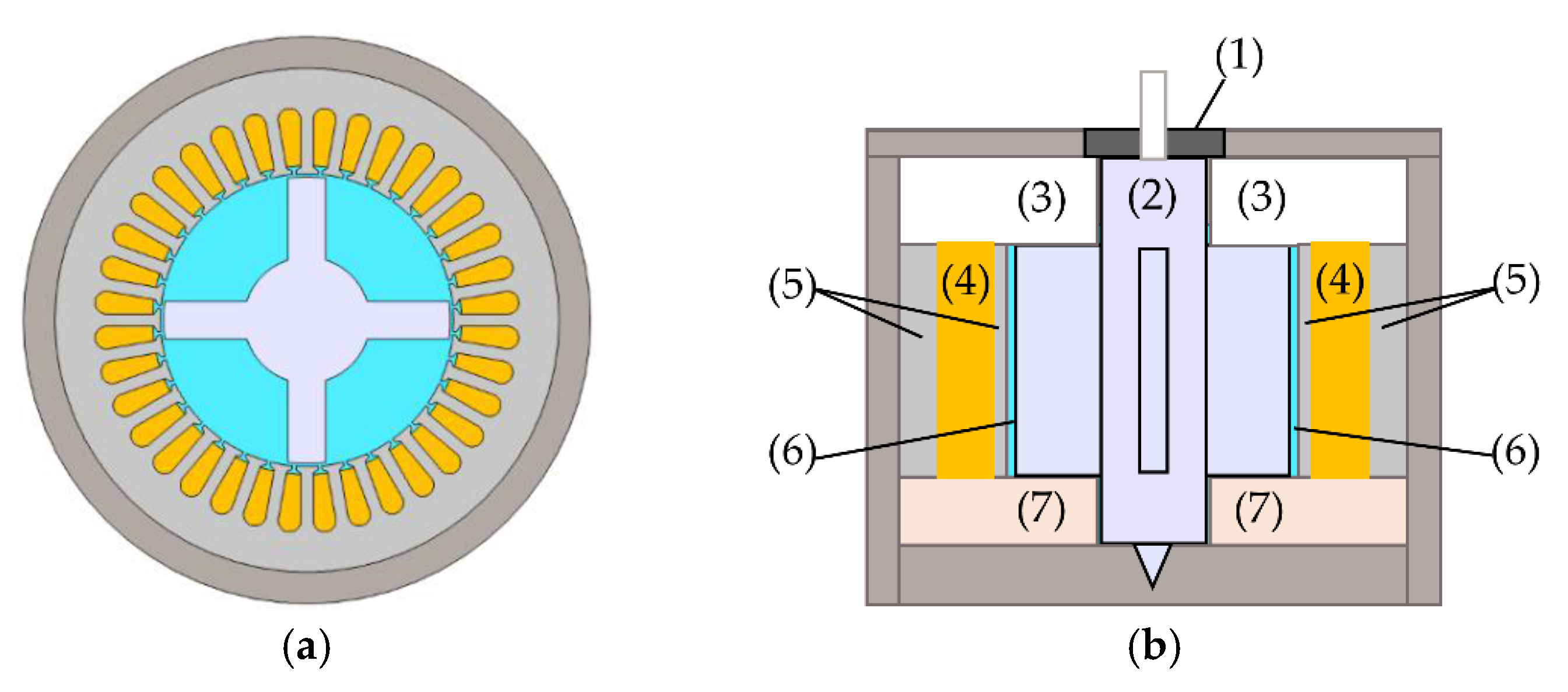
2. Structure of the Experimental Motor for Analysis

Figure 1 shows the structure of the experimental motor. As shown in Figure 1a, the stator and the coil are the same as the reluctance motor, except that the rotor is nonmagnetic. Magnetic fluid fills all the space between the stator and the rotor. The coil area is also slightly filled with the magnetic fluid, but this does not affect the characteristics and safety of the motor. To minimize the amount of magnetic fluid and flux leakage, we placed a nonmagnetic clay under the stator and rotor. The bearing supports the shaft of the rotor. At the bottom, a conical hole is drilled, and some of the magnetic fluid seeps into this hole. Since the magnetic fluid is oil-based, it acts as a lubricant.

3. Controversies of Magnetic Force Density Formula in Magnetic Fluid

Among the magnetic fluid analysis methods, the Navier–Stokes equation method provides the best distributive information. The Navier–Stokes equation (in the incompressible flow) is [1] (pp. 119–122):

$$\rho \left(\frac{\partial v}{\partial t}+v·\nabla v\right)=-\nabla P+f_{\mathrm{mag}}+\eta {\nabla }^{2}v+\rho g$$

(1)

• where $\rho$ is the density.
• $v$ is the fluid velocity vector.
• $P$ is the pressure of fluid.
• $f_{\mathrm{mag}}$ is the magnetic force density vector.
• $\eta$ is the first coefficient of viscosity.
• $g$ is the local acceleration vector due to gravity.

For hydrostatics, let $v=0$ and ignore the gravity. Then, Equation (1) is reduced to

$$0=-\nabla P+f_{\mathrm{mag}}.$$

(2)

Note that $f_{\mathrm{mag}}$ has magnetic fields as variables. When the very-low-frequency electric current flows through the coil set, the magnetostatic equations have the following relations [28] (pp. 139–140):

$$\nabla ·B=0$$

(3–1)

$$\nabla \times H=J_{\mathrm{f}}$$

(3–2)

and its constitutive relation:

$$B={\mu }_{0}H+M$$

(4)

• where $B$ is the magnetic induction field vector.
• $H$ is the magnetic field intensity vector.
• $J_{\mathrm{f}}$ is the free current density vector.
• ${\mu }_0$ is the permeability of vacuum.
• $M$ is the magnetization vector.

The magnetic property of the magnetic fluid is contained in $M$.

Given the $f_{\mathrm{mag}}$ formula, the mechanical pressure distribution in magnetic fluid can be calculated by solving Equation (2). The surface integral of the pressure on the desired object becomes the force or torque due to the pressure. However, it should be noted that the magnetic force density formula is still under controversy. Looking at magnetic density studies historically, several formulas for the magnetic force density have been proposed: Kelvin force density [15], Korteweg–Helmholtz force density [16], and others based on them [17,18,19,20]. Substituting different force density formulas into Equation (1) gives different hydrodynamic phenomena. However, since the magnetic force density is intertwined with numerous physics, it is very difficult to determine the correct solution from it [21,22]. We include the discussions on this issue in the references [23,24,25,26,27].

Conventional electromagnetic force calculation methods are used to obtain the total magnetic force and torque generated by the magnetic material itself. Such methods include the Maxwell stress tensor [29], equivalent magnetic source [30], equivalent magnetizing current [31], and virtual work principle [32]. Among the methods, the virtual work principle can also consider the total outside pressure of the desired objects by differentiating the whole magnetic co-energy.

4. Virtual Work Principle for Torque Analysis

The nonmagnetic rotor has no magnetic force and torque. This rotor generates the torque only from the pressure of the magnetic fluid. This is the output torque of the experimental motor. The magnetic fluid, however, does not transmit all the magnetic force exerted in the fluid to the rotor. It transmits the magnetic force partially to the stator, as well.

The virtual work principle derives a physical quantity through a change of energy in an equilibrium state, through virtual change of some variable. The meaning of virtual is that it is different from the actual change. During the virtual change, we can fix some parameters, such as current density. If the variable is displacement, it derives a force. If it is rotation, it derives a torque. The type of force or torque to be obtained differs depending on what objects are rearranged by virtual displacement or rotation [33]. It should be noted that the application of the virtual work principle to the whole energy includes both the force generated by an object and the force acting outside the object. The outside pressure can also be seen as the result of intertwined physics between magnetic field and hydrostatics.

We first show the process of applying the virtual work principle to the experimental motor. In Figure 2b,c, the rotor is rotating virtually, $\partial \theta$, with respect to ${\theta }_0$. When rotating virtually, not only the rotor but also the magnetic fluid is rearranged together. If the current density in the coil set is fixed, this rearrangement causes a change in B and H, thus also magnetic co-energy. The rotor torque by pressure of the magnetic fluid is as follows:

$${\tau }_{\mathrm{R}}^{\mathrm{pre}}\left({\theta }_0\right)={\frac{\partial W_{\mathrm{m}}^{\mathrm{c}}}{\partial {\theta }_0}\left({\theta }_0\right)|}_{J_{\mathrm{f}}=\mathrm{const}.}$$

(5)

• where, when the rotor angle is ${\theta }_0$,
• ${\tau }_{\mathrm{R}}^{\mathrm{pre}}\left({\theta }_0\right)$ is the rotor torque by pressure of the magnetic fluid at ${\theta }_0$.
• the subscript $J_{\mathrm{f}}=\mathrm{const}.$ means to fix the free current density on all spaces.
• $W_{\mathrm{m}}^{\mathrm{c}}$ is the total magnetic co-energy:

$$W_{\mathrm{m}}^{\mathrm{c}}\left({\theta }_0\right)={{\displaystyle \int }}_{V_{all}}^{}\left({{\displaystyle \int }}_0^{B}H·dB\right)dV$$

(6)

where $V_{all}$ refers to all spaces, including the experimental motor.

Figure 2. Virtual rotation of rotor of the experimental motor for Equation (5), with changes of magnetic flux; (a) the rotor is aligned at ${\theta }_0=0$; (b) before virtual rotation, the rotor is at ${\theta }_0$; (c) after virtual rotation, the rotor is $\partial \theta$ away from ${\theta }_0$ in the CCW direction. The magnetic fluid, B, H, and co-energy also change accordingly. In this process, the current distribution $J_{\mathrm{f},0}$ is fixed. We use these figures in the Section 5 numerical analysis and experiment. Then, $J_{\mathrm{f},0}$ matched input current is used for Section 5, and specifications of the experimental motor are presented in Table A1.

We explain this process in comparison with the case of calculating the total force of an object immersed in water in a gravitational field. An object in water receives two forces: one is its gravity, and the other is the buoyancy, the total object force by pressure in water. Note that the pressure is created by gravity in the water. If the force of the object is derived by using the virtual work principle, it is the sum of its gravity and the buoyancy.

The mathematical structure of the virtual work principle of the magnetic field is similar to the case of the gravitational field. Here, the gravity of the object corresponds to the rotor torque by its magnetic force (if the rotor is made of magnetic material), and the buoyancy corresponds to the rotor torque by pressure of the magnetic fluid. In addition, the gravity density of water corresponds to the magnetic torque density of the magnetic fluid, $f_{\mathrm{mag}}$, but they are not taken into account here. Instead, unlike $f_{\mathrm{mag}}$, the total gravitational energy, $W_{\mathrm{g}}=\left(1/2\right){{\displaystyle \int }}_{V_{\rho }}^{}\rho {\psi }_g dV$ (where $V_{\rho }$ refers to space occupied by $\rho$, $\rho$ is mass density, and ${\psi }_g$ is gravitational potential), and the total magnetic co-energy from Equation (6) are indisputably well known, respectively. Using these total energies, force or torque can be acquired.

Torque calculation using the virtual work principle is not just for the gravity or magnetic force. It yields the sum of all forces that maintain equilibrium for the virtual displacement or rotation [33]. Thus, this method derives, in the gravitational field, the gravity of the object plus the buoyancy, and in the magnetic field, the rotor torque by its magnetic force plus by pressure of the magnetic fluid. If the rotor is nonmagnetic, the rotor receives only pressure from the magnetic fluid. Here, it is unnecessary to know the magnetic force distribution of the magnetic fluid, only the total magnetic co-energy.

5. Numerical Analysis and Experiment

We analyzed numerically and experimented with the experimental motor in Figure 1, made with the specifications shown in Appendix A. Here, we applied a direct current to only one of the three phases. This is to simplify the experiment as much as possible because our purpose is to verify that the virtual work principle in Equation (5) can calculate the output torque of the experimental motor.

In numerical analysis, we used the finite element method to calculate B, H, and the total magnetic co-energy. The magnetic saturation of the iron core and the magnetic fluid was considered [34].

We derived the output torque by approximating Equation (1) as forward difference:

$${\tau }_{\mathrm{R}}^{\mathrm{pre}}\left({\theta }_0\right)\cong {\frac{W_{\mathrm{m}}^{\mathrm{c}}\left({\theta }_0+\Delta \theta \right)-W_{\mathrm{m}}^{\mathrm{c}}\left({\theta }_0\right)}{\Delta \theta }|}_{J_{\mathrm{f}}=\mathrm{const}.}$$

(7)

where $\Delta \theta$ is the approximation value of $\partial \theta$. To do this, we first calculated $W_{\mathrm{m}}^{\mathrm{c}}\left({\theta }_0\right)$ at 1-degree intervals from ${\theta }_0=0$ to 180. In addition, by setting $\Delta \theta =0.1$ degrees, we also calculated $W_{\mathrm{m}}^{\mathrm{c}}\left({\theta }_0+\Delta \theta \right)$. There is almost no difference in torque value in the case of backward and central difference approximation. The solid lines in Figure 3 show these numerical analysis results.

Figure 3. The rotor torque by pressure of the magnetic fluid, that is, the output torque of the experimental motor graph, when the input current is (a) 0.32 A, (b) 0.65 A, (c) 0.97 A. In numerical analysis, the interval is 1 degree. In the experiment, the interval is 3 degrees.

In the experiment, we manufactured the experimental motor as shown in Figure 4, and set up experimental equipment as shown in Figure 5. The iron rod was inserted perpendicularly through the shaft of the motor. This was in contact with the pressure sensor 6.5 cm from the axis. We measured forces applied to the pressure sensor when the rotor was at rest, and repeated it at 3-degree intervals until 180 degrees. Then, we converted forces into torques by multiplying the radius of the rod. The triangular marks in Figure 3 represent the experimental results. Compared to the numerical analysis results, both are well matched. The difference between the two is estimated to be caused by numerical errors, experimental equipment and measurement errors, and the deterioration state of the magnetic fluid in the experiment. This result shows that the output torque calculation for a magnetic fluid-applied motor using the virtual work principle is valid.

Figure 4. Experimental motor: (a) stator; (b) nonmagnetic rotor; (c) experimental motor without magnetic fluid; (d) filled with magnetic fluid.

Figure 5. Equipment setup for measuring the output torque of the experimental motor: (a) overall view; (b) torque measurement iron rod and pressure sensor attached to it.

6. Discussion

6.1. The Significance of Results

In Figure 3, when the input current rises from 0.32 A to 0.65 A, the maximum output torque of the experimental motor is increased by four times. This is the same as the solid reluctance motor when not in saturation. However, when it rises from 0.65 A to 0.97 A, the increase in the maximum output torque is not proportional to the square of the current. This is because as the input current increases, the magnetic fluid is saturated. Relatively, the core is far from the saturation region.

Minimum and maximum output torque occurs when the rotor is positioned at just before 30 and after 60 degrees, respectively. This is because the magnetic fluxes flow more in the 30- and 60-degree teeth than in the others (note that the number of teeth is 36). This means that the change in magnetic fluxes, that is, change of B and H, are greatest just before 30 degrees and after 60 degrees. Thus, by Equation (6), the change of the total magnetic co-energy is also extremized at these angles. As the rotor enters 30 degrees, the output torque is minimized because the nonmagnetic rotor rapidly absorbs a large number of magnetic fluxes and converts them to smaller H. Then, by Equation (6), the total co-energy also decreases most rapidly. The situation is reversed when the rotor escapes from 60 degrees.

Each angle–torque curve in Figure 3 includes an oscillating component. Referring to Figure 2, when the rotor moves near 30 degrees, it moves closer to the current source. From here, up to about 60 degrees, magnetic fluxes are distributions that oscillate as it moves back and forth between teeth and teeth. Then, when the rotor locates this angle domain, the output torque contains an oscillating component. When the rotor exceeds 60 degrees, the magnetic field does not exist in the form of oscillation, and therefore the output torque also becomes a gradual curve.

6.2. Additional Derivations for Stator and Magnetic Fluid

In this subsection, we derive two additional results. For generalization, the rotor is assumed to be a magnetic material. The total rotor torque is

$${\tau }_{\mathrm{R}}^{\mathrm{tot}}\left({\theta }_0\right)={\tau }_{\mathrm{R}}^{\mathrm{mag}}\left({\theta }_0\right)+{\tau }_{\mathrm{R}}^{\mathrm{pre}}\left({\theta }_0\right)$$

(8)

• where, when the rotor angle is ${\theta }_0$,
• ${\tau }_{\mathrm{R}}^{\mathrm{tot}}\left({\theta }_0\right)$ is the total rotor torque.
• ${\tau }_{\mathrm{R}}^{\mathrm{mag}}\left({\theta }_0\right)$ is the rotor torque by its magnetic force.
• ${\tau }_{\mathrm{R}}^{\mathrm{pre}}\left({\theta }_0\right)$ is the rotor torque by pressure of the magnetic fluid.

In this case, the virtual work principle is to calculate ${\tau }_{\mathrm{R}}^{\mathrm{tot}}\left({\theta }_0\right)$. This is because when the rotor is a magnetic material, torques concerned in its virtual rotation are ${\tau }_{\mathrm{R}}^{\mathrm{mag}}\left({\theta }_0\right)$ and ${\tau }_{\mathrm{R}}^{\mathrm{pre}}\left({\theta }_0\right)$. Thus, ${\tau }_{\mathrm{R}}^{\mathrm{tot}}\left({\theta }_0\right)$ is the output torque of the motor that is composed of the magnetic rotor and the magnetic fluid.

The magnetic fluid also applies pressure to the stator. The total stator torque, as in the case of the rotor, is the sum of the contributions of its magnetic force and pressure:

$${\tau }_{\mathrm{S}}^{\mathrm{tot}}\left({\theta }_0\right)={\tau }_{\mathrm{S}}^{\mathrm{mag}}\left({\theta }_0\right)+{\tau }_{\mathrm{S}}^{\mathrm{pre}}\left({\theta }_0\right)$$

(9)

• where, when the rotor angle is ${\theta }_0$,
• ${\tau }_{\mathrm{S}}^{\mathrm{tot}}\left({\theta }_0\right)$ is the total stator torque.
• ${\tau }_{\mathrm{S}}^{\mathrm{mag}}\left({\theta }_0\right)$ is the stator torque by its magnetic force.
• ${\tau }_{\mathrm{S}}^{\mathrm{pre}}\left({\theta }_0\right)$ is the stator torque by pressure of the magnetic fluid.
• ${\tau }_{\mathrm{S}}^{\mathrm{tot}}\left({\theta }_0\right)$ can also be obtained by the virtual work principle, which applies the virtual rotation to the stator; however, if the coordinate system is fixed to the stator, it turns out that the virtual rotation of the stator is the same operation that differs only toward the virtual rotation of the rotor. So,

$${\tau }_{\mathrm{S}}^{\mathrm{tot}}\left({\theta }_0\right)=-{\tau }_{\mathrm{R}}^{\mathrm{tot}}\left({\theta }_0\right).$$

(10)

Equation (10) means that the total stator torque can be directly calculated from Equation (5).

The magnetic fluid torque by its magnetic force is the negative value of the total magnetic force of the remaining parts, according to the law of action–reaction of Lorentz force:

$${\tau }_{\mathrm{F}}^{\mathrm{mag}}\left({\theta }_0\right)=-{\tau }_{\mathrm{S}}^{\mathrm{mag}}\left({\theta }_0\right)-{\tau }_{\mathrm{R}}^{\mathrm{mag}}\left({\theta }_0\right)$$

(11)

where ${\tau }_{\mathrm{F}}^{\mathrm{mag}}\left({\theta }_0\right)$ is the magnetic fluid torque by its magnetic force. Applying Equations (8–10) into (11) gives the following result:

$${\tau }_{\mathrm{F}}^{\mathrm{mag}}\left({\theta }_0\right)={\tau }_{\mathrm{S}}^{\mathrm{pre}}\left({\theta }_0\right)+{\tau }_{\mathrm{R}}^{\mathrm{pre}}\left({\theta }_0\right).$$

(12)

Equation (12) states that when the magnetic fluid receives torque by its magnetic force, it transmits in the form of pressure to the stator and rotor, respectively. Figure 6 shows a plot of ${\tau }_{\mathrm{F}}^{\mathrm{mag}}\left({\theta }_0\right)$, ${\tau }_{\mathrm{S}}^{\mathrm{pre}}\left({\theta }_0\right)$, and ${\tau }_{\mathrm{R}}^{\mathrm{pre}}\left({\theta }_0\right)$, respectively. Note that, using a virtual air gap method [35], it becomes possible to extract the torque by the magnetic force of each part, ${\tau }_{\mathrm{R}}^{\mathrm{mag}}\left({\theta }_0\right)$, ${\tau }_{\mathrm{S}}^{\mathrm{mag}}\left({\theta }_0\right)$, and ${\tau }_{\mathrm{F}}^{\mathrm{mag}}\left({\theta }_0\right)$, separately [36]. Appendix B explains how to calculate the magnetic force by a virtual air gap method.

Figure 6. Magnetic fluid torque by its magnetic force ${\tau }_{\mathrm{F}}^{\mathrm{mag}}\left({\theta }_0\right)$, stator torque by pressure of the magnetic fluid ${\tau }_{\mathrm{S}}^{\mathrm{pre}}\left({\theta }_0\right)$, and rotor torque by pressure of the magnetic fluid ${\tau }_{\mathrm{R}}^{\mathrm{pre}}\left({\theta }_0\right)$ of the experimental motor, according to rotor angle. Input current is 0.97 A.

7. Conclusions

The purpose of our paper was to find an approach to calculate the force and torque of a desired object immersed in the magnetic fluid. When the magnetic force density is used as a forcing term, solving the Navier–Stokes equation directly raises a problem of reliability because the most important forcing term, the magnetic force density, is still under controversy. To resolve this problem, this paper showed that the calculation of the torque of these applications should not only use the magnetic force calculation method, but also consider the mechanical pressure using an indirect approach, such as the virtual work principle. To illustrate this, we devised and created an experimental motor composed of a nonmagnetic rotor immersed in a magnetic fluid. If the virtual work principle is applied by differentiating the whole magnetic co-energy, it can calculate the nonmagnetic rotor torque received by pressure of the magnetic fluid. The comparison between numerical and experimental analysis shows its validity. Further discussion also shows the case of the stator, and reveals the origin of stator and rotor torque by pressure. Our future work is to apply this approach to the motors having the rotor of magnetic materials.

References

- Rosensweig, R.E. Ferrohydrodynamics; Dover Publications, Inc.: Mineola, NY, USA, 1997. [Google Scholar]
- Raj, K.; Moskowitz, B.; Casciari, R. Advances in ferrofluid technology. J. Magn. Magn. Mater. 1995, 149, 174–180. [Google Scholar] [CrossRef]
- Scherer, C.; Neto, A.M.F. Ferrofluids: Properties and applications. Braz. J. Phys. 2005, 35, 718–727. [Google Scholar] [CrossRef]
- Torres-Diaz, I.; Rinaldi, C. Recent progress in ferrofluids research: Novel applications of magnetically controllable and tunable fluids. Soft Matter 2014, 10, 8584–8602. [Google Scholar] [CrossRef] [PubMed]
- Zhang, X.; Sun, L.; Yu, Y.; Zhao, Y. Flexible Ferrofluids: Design and Applications. Adv. Mater. 2019, 31, e1903497. [Google Scholar] [CrossRef] [PubMed]
- Sohail, A.; Fatima, M.; Ellahi, R.; Akram, K.B. A videographic assessment of ferrofluid during magnetic drug targeting: An application of artificial intelligence in nanomedicine. J. Mol. Liq. 2019, 285, 47–57. [Google Scholar] [CrossRef]
- Mody, V.V.; Cox, A.G.; Shah, S.; Singh, A.; Bevins, W.; Parihar, H. Magnetic nanoparticle drug delivery systems for targeting tumor. Appl. Nanosci. 2013, 4, 385–392. [Google Scholar] [CrossRef]
- Hatch, A.; Kamholz, A.; Holman, G.; Yager, P.; Bohringer, K. A ferrofluidic magnetic micropump. J. Microelectromech. Syst. 2001, 10, 215–221. [Google Scholar] [CrossRef]
- Chitnis, G.; Ziaie, B. A ferrofluid-based wireless pressure sensor. J. Micromech. Microeng. 2013, 23. [Google Scholar] [CrossRef]
- Kurtoğlu, E.; Bilgin, A.; Şeşen, M.; Mısırlıoğlu, B.; Yıldız, M.; Acar, H.F.Y.; Koşar, A. Ferrofluids actuation with varying magnetic fluids for micropumping applications. Microfluid. Nanofluid. 2012, 13, 683–694. [Google Scholar] [CrossRef]
- Engelmann, S.; Nethe, A.; Scholz, T.h.; Stahlmann, H.-D. Concept of a new type of electric machines using ferrofluids. J. Magn. Magn. Mater. 2005, 293, 685–689. [Google Scholar] [CrossRef]
- Zeng, G.; Xiang-Yu, Y.; Yin, H.; Pei, Y.; Zhao, S.; Cao, J.; Qiu, L. Asynchronous Machine with Ferrofluid in Gap: Modeling, Simulation, and Analysis. IEEE Trans. Magn. 2019, 56, 1–4. [Google Scholar] [CrossRef]
- Engelmann, S.; Nethe, A.; Scholz, T.; Stahlmann, H.-D. Experiments with a ferrofluid-supported linear electric motor. Appl. Organomet. Chem. 2004, 18, 529–531. [Google Scholar] [CrossRef]
- Yang, I.-J.; Song, S.-W.; Kim, D.-H.; Kim, K.-S.; Kim, W.-H. Improvement in Torque Density by Ferrofluid Injection into Magnet Tolerance of Interior Permanent Magnet Synchronous Motor. Energies 2021, 14, 1736. [Google Scholar] [CrossRef]
- Livens, G.H. The Theory of Electricity; Cambridge University Press: Cambridge, UK, 1918; pp. 212–220. [Google Scholar]
- Stratton, J.A. Electromagnetic Theory; McGraw-Hill: New York, NY, USA, 2015. [Google Scholar] [CrossRef]
- Chu, L.; Haus, H.; Penfield, P. The force density in polarizable and magnetizable fluids. Proc. IEEE 1966, 54, 920–935. [Google Scholar] [CrossRef]
- Landau, L.D.; Pitaevskii, L.P.; Lifshitz, E.M. Electrodynamics of Continuous Media, 2nd ed.; Butterworth-Heinemann: Oxford, UK, 1984; p. 127. [Google Scholar]
- Mansuripur, M. Electromagnetic stress tensor in ponderable media. Opt. Express 2008, 16, 5193–5198. [Google Scholar] [CrossRef]
- Shevchenko, A.; Hoenders, B.J. Microscopic derivation of electromagnetic force density in magnetic dielectric media. New J. Phys. 2010, 12. [Google Scholar] [CrossRef]
- Penfield, P.; Haus, H.A. Electrodynamics of Moving Media; The MIT Press: Cambridge, MA, USA, 1968; pp. 75–77. [Google Scholar] [CrossRef]
- Bobbio, S. Electrodynamics of Materials; Academic Press: San Diego, CA, USA, 2000. [Google Scholar]
- Odenbach, S.; Liu, M. Invalidation of the Kelvin Force in Ferrofluids. Phys. Rev. Lett. 2001, 86, 328–331. [Google Scholar] [CrossRef]
- Rinaldi, C.; Brenner, H. Body versus surface forces in continuum mechanics: Is the Maxwell stress tensor a physically objective Cauchy stress? Phys. Rev. E 2003, 65, 036615. [Google Scholar] [CrossRef]
- Bethune-Waddell, M.; Chau, K.J. Simulations of radiation pressure experiments narrow down the energy and momentum of light in matter. Rep. Prog. Phys. 2015, 78, 122401. [Google Scholar] [CrossRef]
- Mansuripur, M. Force, torque, linear momentum, and angular momentum in classical electrodynamics. Appl. Phys. A 2017, 123, 653. [Google Scholar] [CrossRef]
- Reich, F.A.; Rickert, W.; Müller, W.H. An investigation into electromagnetic force models: Differences in global and local effects demonstrated by selected problems. Contin. Mech. Thermodyn. 2017, 30, 233–266. [Google Scholar] [CrossRef]
- Panofsky, W.K.H.; Phillips, M.; Morse, P.M. Classical Electricity and Magnetism; Dover Publications, Inc.: Mineola, NY, USA, 1956; pp. 22–24. [Google Scholar] [CrossRef]
- Reichet, K.; Freundl, H.; Vogt, W. The calculation of forces and torques within numerical magnetic field calculation methods. Proc. Compumag. 1976, 76, 64–74. [Google Scholar]
- Bobbio, S.; Girdinio, P.; Molfino, P.; Delfino, F. Equivalent sources methods for the numerical evaluation of magnetic force with extension to nonlinear materials. IEEE Trans. Magn. 2000, 36, 663–666. [Google Scholar] [CrossRef]
- Kabashima, T.; Kawahara, A.; Goto, T. Force calculation using magnetizing currents. IEEE Trans. Magn. 1988, 24, 451–454. [Google Scholar] [CrossRef]
- Coulomb, J.C.; Meunier, G.; Sabonnadiere, J.C. An original stationary method using local jacobian derivative for direct finite element computation of electromechanical force, torque and siftness. J. Magn. Magn. Mater. 1982, 26, 337–339. [Google Scholar] [CrossRef]
- Reddy, J.N. Energy Principles and Variational Methods in Applied Mechanics, 3rd ed.; John Wiley & Sons, Inc.: Hoboken, NJ, USA, 2017; p. 131. [Google Scholar]
- Jiles, D. Introduction to Magnetism and Magnetic Materials, 3rd ed.; CRC Press: Boca Raton, FL, USA, 2015; pp. 99–102. [Google Scholar]
- Choi, H.-S.; Park, I.-H.; Lee, S.-H. Electromagnetic body force calculation based on virtual air gap. J. Appl. Phys. 2006, 99, 08H903. [Google Scholar] [CrossRef]
- Choi, H.S.; Kim, Y.S.; Lee, J.H.; Park, I.H. An Observation of Body Force Distributions in Electric Machines. IEEE Trans. Magn. 2007, 43, 1861–1864. [Google Scholar] [CrossRef]
- Choi, H.S.; Park, I.H.; Lee, S.H. Concept of virtual air gap and its applications for force calculation. IEEE Trans. Magn. 2006, 42, 663–666. [Google Scholar] [CrossRef]
- Choi, H.S.; Park, I.H.; Lee, S.H. Force Calculation of Magnetized Bodies in Contact Using Kelvin’s Formula and Virtual Air-Gap. IEEE Trans. Appl. Supercond. 2006, 16, 1832–1835. [Google Scholar] [CrossRef]
- Choi, H.S.; Lee, S.H.; Kim, Y.S.; Kim, K.T.; Park, I.H. Implementation of Virtual Work Principle in Virtual Air Gap. IEEE Trans. Magn. 2008, 44, 1286–1289. [Google Scholar] [CrossRef]
- Park, B.S.; Choi, H.S.; Park, J.O.; Wang, J.H.; Park, I.H. Equality of the Kelvin and Korteweg–Helmholtz Force Densities Inside Dielectric Materials. IEEE Trans. Magn. 2020, 56, 4. [Google Scholar] [CrossRef]
- Kemp, B.A. Resolution of the Abraham-Minkowski debate: Implications for the electromagnetic wave theory of light in matter. J. Appl. Phys. 2011, 109, 111101. [Google Scholar] [CrossRef]
- Frias, W.; Smolyakov, A.I. Electromagnetic forces and internal stresses in dielectric media. Phys. Rev. E 2012, 85, 046606. [Google Scholar] [CrossRef] [PubMed]
- Mahdy, M.R.C.; Gao, D.; Ding, W.; Mehmood, M.Q.; Nieto-Vesperinas, M.; Qui, C.-W. A unified theory correcting Einstein-Laub electrodynamics solves dilemmas in the photon momenta and electromagnetic stress tensors. arXiv 2015, arXiv:1509.06971. [Google Scholar]
- Kemp, B.A.; Sheppard, C.J. Electromagnetic and material contributions to stress, energy, and momentum in metamaterials. Adv. Electromagn. 2017, 6, 11–19. [Google Scholar] [CrossRef][Green Version]
Publisher’s Note: MDPI stays neutral with regard to jurisdictional claims in published maps and institutional affiliations. |
© 2021 by the authors. Licensee MDPI, Basel, Switzerland. This article is an open access article distributed under the terms and conditions of the Creative Commons Attribution (CC BY) license (https://creativecommons.org/licenses/by/4.0/).