Closed-Form Expressions to Estimate the Mean and Variance of the Total Vector Error

Abstract

The need for accurate measurements and for estimating the uncertainties associated with measures are two pillars for researchers and metrologists. This is particularly true in distribution networks due to a mass deployment of new intelligent electronic devices. Among such devices, phasor measurement units are key enablers for obtaining the full observability of the grid. The phasor measurement unit performance is mostly evaluated by means of the total vector error, which combines the error on amplitude, phase, and time. However, the total vector error is typically provided merely as a number, that could vary within an unknown interval. This may result into the phasor measurement unit incompliance with the final user expectancies. To this purpose, and with the aim of answering practical needs from the industrial world, this paper presents a closed-form expression that allows us to quantify, in a simple way, the confidence interval associated with the total vector error. The input required by the expression is the set of errors that typically affects the analog to digital converter of a phasor measurement unit. The obtained expression has been validated by means of the Monte Carlo method in a variety of realistic conditions. The results confirm the applicability and effectiveness of the proposed expression. It can be then easily implemented in all monitoring device algorithms, or directly by the manufacturer to characterize their devices, to solve the lack of knowledge that affects the total vector error computation.

1. Introduction

The digitalization of the power network is becoming a priority for electric utilities and system operators (SOs). Of course, the transmission and distribution portions of the network (TN and DN) have different rates of digitalization due to their different topology and due to the available investments per node of the grid. The two actors that are leading this innovation process are as follows: the new generation of instrument transformers (ITs), also referred to as low-power instrument transformers (LPITs) or non-conventional instrument transformers (NCITs), and the intelligent electronic devices (IEDs).

Starting with the LPITs, they have brought a lot of benefits and new features to the measurement of voltages and currents [1,2,3]. For example, they are smaller and lighter compared to the bulky legacy ITs. Furthermore, they feature higher immunity towards external influence factors, and they are easier to install in those sites where there is limited space for additional equipment. As their name implies, their output never exceeds a few voltampere, which make them suitable for being directly connected to the analog-to-digital converters (ADC) of the typical acquisition systems. Finally, considering the increasing interest of power quality (PQ) evaluation, LPITs typically have wider bandwidth compared to the older technologies.

Turning to the standard perspective, LPITs can be found inside the IEC 61869 series. In particular IEC 61869-6 [4] describes general aspects on their operation and limits, whereas documents −10 and −11 [5,6] specifically treat the current and voltage versions of the LPITs, referred to as low-power current transformers (LPCTs) and low-power voltage transformers (LPVTs), respectively.

The second main actor of the digitalization, as mentioned before, is the IED. In fact, a variety of measurement instruments are being deployed in the DNs to collect the quantities and the information necessary to improve the control and the management of the grid. Among the IEDs there are: energy meters, smart protection devices, merging units (MUs) and waveform recorders like the well-known phasor measurement units (PMUs).

PMUs are the core of this work. As a matter of fact, their spread among the DN started slowly a couple of decades ago [7] and is increasing daily as it has been documented in [8,9]. The added value of a PMU, as detailed in Section 2, is the possibility to associate a time stamp, hence to synchronize the voltage and current measurements at each node of the network with a reference time signal (typically the GPS). In fact, in case of loss of synchronization [10,11,12,13,14], the PMU downgrades to an instrument with the same capabilities of a legacy meter, without any added value (de facto, a PMU consists of an ADC plus a GPS plus an intelligent device that performs the required operations on the samples).

PMUs, like all instruments and sensors, are affected by an uncertainty. This can be distinguished between the contribution due to the intrinsic components inside the PMU, and the contribution due to the sensors adopted to measure voltages and currents that propagates up to the PMU’s output. Therefore, the PMU’s uncertainty affects all the parameters computed from its measured data. Among these, the total vector error (TVE) is a significant parameter that is used to assess the performance of a PMU in both static and dynamic conditions. However, it is really difficult to find (i) any PMU manufacturer giving the range of variation of the TVE. In fact, each PMU, despite having all the hardware with the same nominal characteristics, features a specific TVE value, different from the others, and (ii) any document within the literature estimating the range of variation of TVE (except for the standard deviation obtained from the repeated measurements of the parameter).

In light of the above, authors in this paper formulate a closed-form expression that associates a mean value and a variance to the TVE, considered as a random variable (RV). The expressions are obtained starting from the typical factors affecting the collected waveforms and due to the PMU’s hardware (non-linearity, offset, gain, delay, etc.).

Of course, literature does treat the uncertainties affecting the PMU and its parameters. For example, [15] adopts the Monte Carlo method (MCM) and the TVE to assess an algorithm for the phasor extraction. The role of disturbances, affecting the analog input of a PMU, on the frequency and rate of change of frequency (ROCOF) computation is discussed in [16]. How noise influences the power frequency extraction is detailed in [17]. In [18] a simulator of PMU has been developed to model its uncertainties by means of the MCM. An interesting study on the limits of using TVE in the PMU’s performance assessment is presented in [19]. The accuracy of the PMU’s measurements, focusing on the phase and time synchronization requirements is treated in [20,21], respectively. Finally, the uncertainty evaluation in case of state estimation or in case of loss of synchronization is treated in [22,23], respectively.

However, despite the amount of literature on the topic, to the authors’ knowledge, there is a lack of material on how to estimate the range of variation of the TVE. The importance of filling this gap consists of the fact that the TVE is used to accept or deny the measures performed by a PMU. Therefore, it is critical to know how well the actual TVE matches the rated one. Furthermore, considering that the intrinsic uncertainty contributions adopted here are provided by the manufacturer, the outcome of this work may be used by them to increase the information given to the final user.

Consequently, authors started from their previous experience on evaluating the uncertainty of typical parameters (THD [24] and residual voltage [25]) to obtain the TVE mean and variance.

It can be concluded that the added value of this work is to provide a simple expression that allows the quantification of the TVE mean and variance. The two expressions will help (i) PMUs producers to better quantify the goodness of the TVE that has been measured during the PMU testing, (ii) final users for better assessing the TVE results when the PMU measurements are involved, (iii) SOs to better assess the PMUs that are going to be installed in their networks. Furthermore, the found expressions may then be included in all PMUs (or their calibrators).

The remainder of this work is structured as follows. Section 2 contains a brief overview of the PMU technology and on the TVE. The mathematic development necessary to obtain the closed-form expression of the mean and standard deviation of the TVE is described in Section 3. The validation of what is obtained, through the MCM, is described in Section 4. Finally, the main achievements and conclusion are contained in Section 5.

2. PMU and Total Vector Error

The concept of phasor, on which the PMU is based, was firstly introduced by Proteus Steinmetz in 1916 [26]. Nowadays, the PMU is standardized in the document IEC 60255-118-1 [27], where it is defined as a “device or function in a multifunction device that produces synchronized phasor, frequency, and rate of change of frequency estimates from voltage and/or current signals and a time synchronizing signal”. In [27] the phasor is defined as “complex equivalent of a sinusoidal wave quantity such that the complex modulus is the cosine wave amplitude, and the complex angle (in polar form) is the cosine wave phase angle”. The meaning of phasor is then enhanced when the concept of synchronization is introduced to explain the functionalities of a PMU. Therefore, a synchrophasor is a “phasor representing the fundamental of an AC signal whose magnitude is the RMS value of the fundamental amplitude and angle is the difference between the signal fundamental angle and the phase angle of a cosine at the nominal signal frequency that is synchronized to UTC time” [27]. Furthermore, the generic synchrophasor X can be written as:

$$X\left(t\right)=\left(\frac{X_m\left(t\right)}{\sqrt{2}},\varphi \left(t\right)\right)$$

(1)

where $X_m$(t) is the peak magnitude of the sinusoidal signal and $\varphi$(t) is the phase difference between the angular position and the phase due to the nominal frequency of the signal.

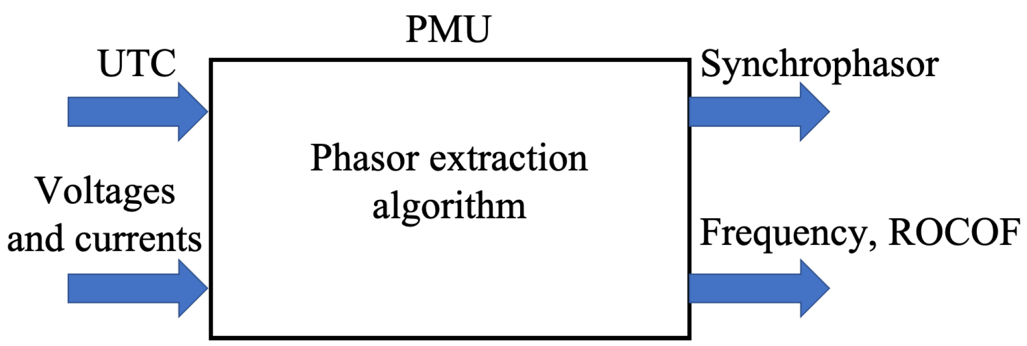
Overall, Figure 1 summarizes the working principle of a PMU. As it is clear from the figure, the PMU receives the current and voltage waveforms as inputs, plus the UTC time. This allows a time stamp to be associated with each synchrophasor produced by the PMU.

The reporting rate of a PMU defines how many times in a second the synchrophasor, the frequency, and the ROCOF are provided to the data concentrator. In [27] the minimum is defined, as well as the suggested reporting rates that a PMU shall comply with (from 10 to 100 frames per second in the case of a 50 Hz system). The synchrophasor is then evaluated through the TVE, which is defined as:

$$TVE\left(m\right)=\sqrt{\frac{{\left({\widehat{X}}_r\left(m\right)-X_r\left(m\right)\right)}^2+{\left({\widehat{X}}_i\left(m\right)-X_i\left(m\right)\right)}^2}{{\left(X_r\left(m\right)\right)}^2+{\left(X_i\left(m\right)\right)}^2}}$$

(2)

where $m$ indicates the report number, $X_r\left(m\right)$ and $X_i\left(m\right)$ are the real and imaginary parts of the reference value, whereas ${\widehat{X}}_r\left(m\right)$ and ${\widehat{X}}_i\left(m\right)$ are the real and imaginary parts of the PMU estimates.

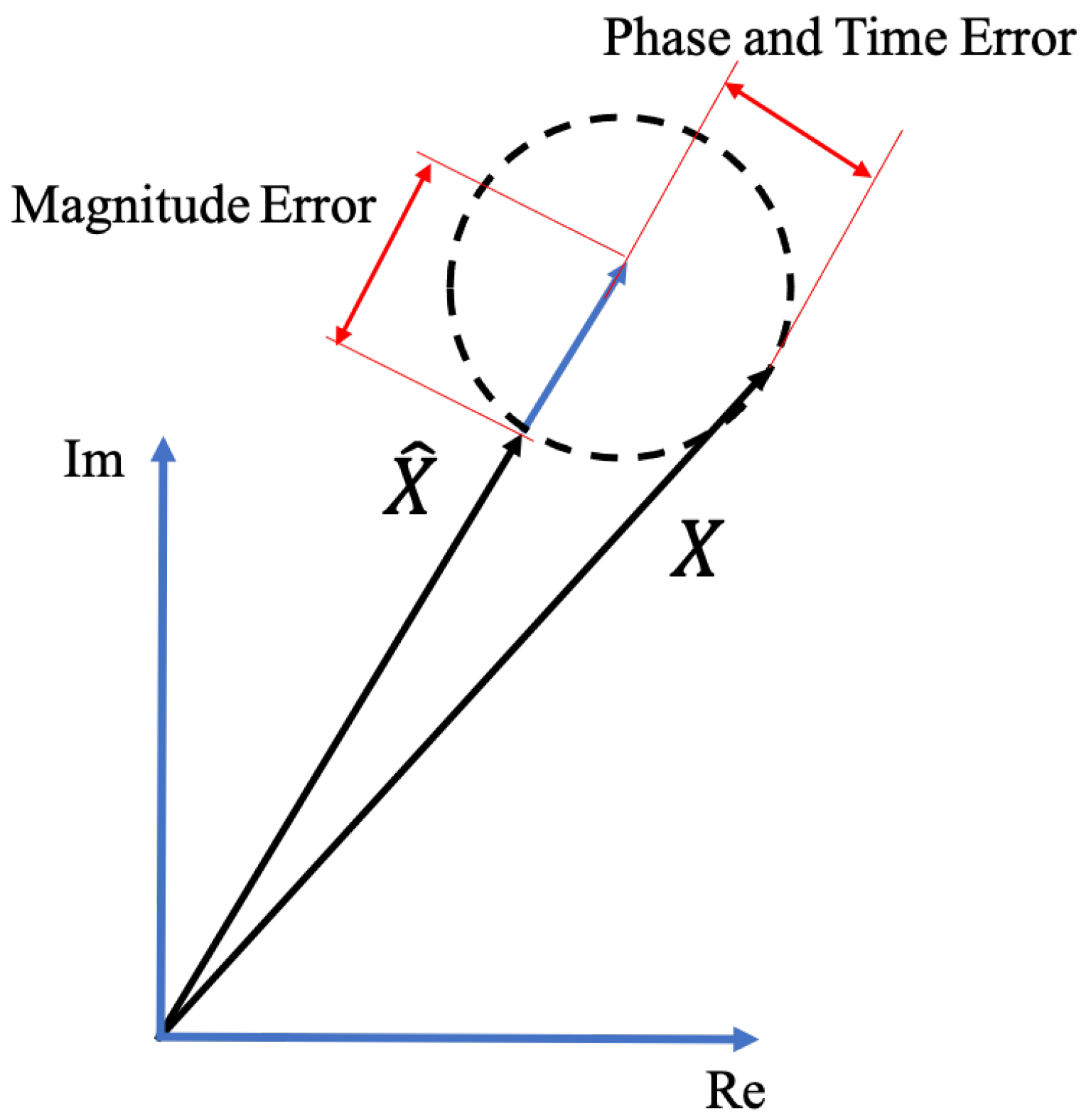
It is worth highlighting that the TVE is a parameter that blends the three sources of error that affect the PMU measurements. As it is clarified in Figure 2, the three sources of error are magnitude, phase, and the time synchronization error.

The fact of combining all the error sources might be seen either positively or negatively, depending on the perspective. It could be positive if the interest is on the overall performance of the PMU (accept or deny the measurements). On the contrary, using the TVE becomes less significant when the PMU must be characterized, and the single sources of error must be quantified.

3. Mean and Variance Estimation

After the brief introduction on the PMUs and TVE given in the previous section, this section details the mathematic steps necessary to formulate the problem under investigation and its resolution. Section 3.1 presents the idea underlying the work, whereas Section 3.2 contains the process that allows the finding of the mean value and variance of the TVE.

3.1. Problem Definition

The starting point of this study is (2), the definition of TVE. Such an expression uses the real and imaginary part of the power system frequency component extracted from an analog signal. Therefore, it is important to begin the analysis from the inputs that a PMU receives. Note that, in this study, no distinguish between the steady-state and the dynamic nature of the input signal is considered. This is because the analysis of the TVE is based on assumptions independent of the input signal, which of course might be ideal or distorted, static or dynamic.

Let’s define $x$ a generic sequence of $N$ elements, measured either with a current or a voltage sensor, which is the input of the ADC of the PMU. Afterwards, $x$ is corrupted by the errors introduced by the ADC, namely: the gain error $G$, the offset $O$, the nonlinearity error $L$, the noise $R$, and the phase delay $\mathsf{\Delta }\psi$, which can be considered the overall term that includes all time and phase delays (e.g., the UTC). Such error contributes can be considered uniformly distributed, as detailed in Section 3.2. This choice is motivated by the fact that the manufacturers of ADC almost never provide the probability density function (pdf) associated to the accuracy parameters of their products (it is rare, but if it is provided the following method can be easily adapted). Therefore, according to the Guide to the Expression of Uncertainty in Measurements (GUM) [28] the worst case must be used: the random variable must be considered as uniformly distributed when no other information is available. However, the study presented here might be customized by the final user depending on the information available. Therefore, the obtained results can be considered the output of the worst and most general case.

The generic element of the corrupted sequence $\widehat{x}$, output of the ADC, can then be written as:

$$\widehat{x}\left(n\right)=\left(x\left(n\right)+gx\left(n\right)+o+l\left(n\right)x_{FS}+r\left(n\right)\right)e^{-i\mathsf{\Delta }\psi }$$

(3)

where $n$ is the element counter, $x$ is the ideal sample, and $g$, $o$, $l$, $r$, and $\psi$ are the generic elements of the distributions of which $G$, $O$, $L$, $R$, and $\mathsf{\Delta }\psi$ represent the extremes, respectively. Finally, $x_{FS}$ is the ADC full scale and $i$ is the complex operator.

To obtain the desired phasor, the next step is the application of the discrete Fourier transform (DFT) (which is the most common among several filters that can be applied to the signal to extract the phasor) to $\widehat{x}$:

$$\widehat{X}\left(k\right)=\frac{1}{N}{\displaystyle {\displaystyle \sum }_{n=0}^{N-1}}\left(x\left(n\right)+gx\left(n\right)+o+l\left(n\right)x_{FS}+r\left(n\right)\right)e^{-i2\pi nk/N}{e}^{-i\mathsf{\Delta }\psi }$$

(4)

which in the case of considering one period ($k=1$), for the sake of simplicity but without loss of generality, becomes:

$$\widehat{X}=\left(X+gX+\frac{x_{FS}}{N}{\displaystyle {\displaystyle \sum }_{n=0}^{N-1}}\left(l\left(n\right)\right)e^{-i2\pi n/N}+\frac{1}{N}{\displaystyle {\displaystyle \sum }_{n=0}^{N-1}}\left(r\left(n\right)\right)e^{-i2\pi n/N}\right)e^{-i\mathsf{\Delta }\psi }$$

(5)

Two simple comments arise from (5): (i) after the application of the DFT the offset term disappears; (ii) moving from (4) to (5) it becomes clear which sources of error remain constant for the entire sequence ($g$ and $\mathsf{\Delta }\psi$), and which vary from sample to sample ($l$ and $r$). A small note on this comment: the assumptions used to write (5) are based on the datasheets of common ADC adopted in the measurement field. Therefore, our aim is not to confute or to verify if the behavior of the given parameters differs from what is specified.

Equation (5) can be rewritten explicating the sine and cosine terms by means of the Euler expression:

$$\widehat{X}=\left(X+gX+\frac{x_{FS}}{N}{\displaystyle {\displaystyle \sum }_{n=0}^{N-1}}\left(l\left(n\right)\right)e^{-i2\pi n/N}+\frac{1}{N}{\displaystyle {\displaystyle \sum }_{n=0}^{N-1}}\left(r\left(n\right)\right)e^{-i2\pi n/N}\right)\left(\cos \mathsf{\Delta }\psi +i\sin \mathsf{\Delta }\psi \right)$$

(6)

By considering that the error contributes are very small, let us assume that the product of two of them is negligible (e.g., $gXsin\mathsf{\Delta }\psi$) when the sine is involved. In the case of the cosines, they are approximated with 1. The result is:

$$\widehat{X}=X\cos \mathsf{\Delta }\psi +iX\sin \mathsf{\Delta }\psi +gX+\frac{x_{FS}}{N}{\displaystyle {\displaystyle \sum }_{n=0}^{N-1}}\left(l\left(n\right)\right)e^{-i2\pi nk/N}+\frac{1}{N}{\displaystyle {\displaystyle \sum }_{n=0}^{N-1}}\left(r\left(n\right)\right)e^{-i2\pi nk/N}$$

(7)

Considering the numerator of the TVE in (2), the measured $\widehat{X}$ must be subtracted by the ideal or reference phasor $X$, obtaining:

$$\mathsf{\Delta }\widehat{X}=X\left(\cos \mathsf{\Delta }\psi +i\sin \mathsf{\Delta }\psi +g-1\right)+\frac{x_{FS}}{N}{\displaystyle {\displaystyle \sum }_{n=0}^{N-1}}\left(l\left(n\right)\right)e^{-i2\pi n/N}+\frac{1}{N}{\displaystyle {\displaystyle \sum }_{n=0}^{N-1}}\left(r\left(n\right)\right)e^{-i2\pi n/N}$$

(8)

The second hypothesis that is introduced consists of considering the ideal phasor constituted only by a real component $X=X+i0$. Such a choice does not affect the computation, but it simplifies the study. Furthermore, the ideal phasor is selected by the algorithm developer; hence, the choice of a real phasor is completely reasonable.

From (8) it is possible to separate the real and imaginary parts as:

$$\begin{array}{c}Re\left\{\mathsf{\Delta }\widehat{X}\right\}={\widehat{X}}_r-X_r={\widehat{X}}_r-X=X\left(\cos \mathsf{\Delta }\psi +g-1\right)+\hfill \\ \frac{x_{FS}}{N}{\displaystyle {\displaystyle \sum }_{n=0}^{N-1}}\left(l\left(n\right)\right)\cos \left(2\pi n/N\right)+\frac{1}{N}{\displaystyle {\displaystyle \sum }_{n=0}^{N-1}}\left(r\left(n\right)\right)\cos \left(2\pi n/N\right)\hfill \end{array}$$

(9)

$$\begin{array}{c}Im\left\{\mathsf{\Delta }\widehat{X}\right\}={\widehat{X}}_i-X_i={\widehat{X}}_i=X\sin \mathsf{\Delta }\psi +\hfill \\ \frac{x_{FS}}{N}{\displaystyle {\displaystyle \sum }_{n=0}^{N-1}}\left(l\left(n\right)\right)\sin \left(2\pi n/N\right)+\frac{1}{N}{\displaystyle {\displaystyle \sum }_{n=0}^{N-1}}\left(r\left(n\right)\right)\sin \left(2\pi n/N\right)\hfill \end{array}$$

(10)

By squaring (9) and (10) one obtains the addends of the numerator of (2).

$$\begin{array}{c}Re{\left\{\mathsf{\Delta }\widehat{X}\right\}}^2=X^2{\left(\cos \mathsf{\Delta }\psi +g-1\right)}^2+{\left(\frac{x_{FS}}{N}{\displaystyle {\displaystyle \sum }_{n=0}^{N-1}}\left(l\left(n\right)\right)\cos \left(\frac{2\pi n}{N}\right)\right)}^2\hfill \\ +{\left(\frac{1}{N}{\displaystyle {\displaystyle \sum }_{n=0}^{N-1}}\left(r\left(n\right)\right)\cos \left(\frac{2\pi n}{N}\right)\right)}^2+2X\left(\cos \mathsf{\Delta }\psi +g-1\right)\hfill \\ \frac{x_{FS}}{N}{\displaystyle {\displaystyle \sum }_{n=0}^{N-1}}\left(l\left(n\right)\right)\cos \left(\frac{2\pi n}{N}\right)+2X\left(\cos \mathsf{\Delta }\psi +g-1\right)\frac{1}{N}{\displaystyle {\displaystyle \sum }_{n=0}^{N-1}}\left(r\left(n\right)\right)\cos \left(\frac{2\pi n}{N}\right)\hfill \\ +2\frac{x_{FS}}{N}{\displaystyle {\displaystyle \sum }_{n=0}^{N-1}}\left(l\left(n\right)\right)\cos \left(2\pi n/N\right)\frac{1}{N}{\displaystyle {\displaystyle \sum }_{n=0}^{N-1}}\left(r\left(n\right)\right)\cos \left(2\pi n/N\right)\hfill \end{array}$$

(11)

$$\begin{array}{c}Im{\left\{\mathsf{\Delta }\widehat{X}\right\}}^2=X^2{\left(\sin \mathsf{\Delta }\psi \right)}^2+{\left(\frac{x_{FS}}{N}{\displaystyle {\displaystyle \sum }_{n=0}^{N-1}}\left(l\left(n\right)\right)\sin \left(\frac{2\pi n}{N}\right)\right)}^2\hfill \\ +{\left(\frac{1}{N}{\displaystyle {\displaystyle \sum }_{n=0}^{N-1}}\left(r\left(n\right)\right)\sin \left(\frac{2\pi n}{N}\right)\right)}^2+2X\frac{x_{FS}}{N}\sin \mathsf{\Delta }\psi {\displaystyle {\displaystyle \sum }_{n=0}^{N-1}}\left(l\left(n\right)\right)\sin \left(\frac{2\pi n}{N}\right)\hfill \\ +\frac{2X\sin \mathsf{\Delta }\psi }{N}{\displaystyle {\displaystyle \sum }_{n=0}^{N-1}}\left(r\left(n\right)\right)\cos \left(\frac{2\pi n}{N}\right)+\hfill \\ 2\frac{x_{FS}}{N}{\displaystyle {\displaystyle \sum }_{n=0}^{N-1}}\left(l\left(n\right)\right)\sin \left(2\pi n/N\right)\frac{1}{N}{\displaystyle {\displaystyle \sum }_{n=0}^{N-1}}\left(r\left(n\right)\right)\sin \left(2\pi n/N\right)\hfill \end{array}$$

(12)

As a final hypothesis let us assume to approximate all terms with $sin\mathsf{\Delta }\psi$ with the angle $\mathsf{\Delta }\psi$ and the terms with $cos\mathsf{\Delta }\psi$ with 1. This way, (11) and (12) are simplified as:

$$\begin{array}{c}Re{\left\{\mathsf{\Delta }\widehat{X}\right\}}^2={\left(Xg\right)}^2+{\left(\frac{x_{FS}}{N}{\displaystyle {\displaystyle \sum }_{n=0}^{N-1}}\left(l\left(n\right)\right)\cos \left(\frac{2\pi n}{N}\right)\right)}^2\hfill \\ +{\left(\frac{1}{N}{\displaystyle {\displaystyle \sum }_{n=0}^{N-1}}\left(r\left(n\right)\right)\cos \left(\frac{2\pi n}{N}\right)\right)}^2+\frac{2Xg{x}_{FS}}{N}{\displaystyle {\displaystyle \sum }_{n=0}^{N-1}}\left(l\left(n\right)\right)\cos \left(\frac{2\pi n}{N}\right)\hfill \\ +\frac{2Xg}{N}{\displaystyle {\displaystyle \sum }_{n=0}^{N-1}}\left(r\left(n\right)\right)\cos \left(\frac{2\pi n}{N}\right)+\hfill \\ \frac{2x_{FS}}{N^2}{\displaystyle {\displaystyle \sum }_{n=0}^{N-1}}\left(l\left(n\right)\right)\cos \left(2\pi n/N\right){\displaystyle {\displaystyle \sum }_{n=0}^{N-1}}\left(r\left(n\right)\right)\cos \left(2\pi n/N\right)\hfill \end{array}$$

(13)

$$\begin{array}{c}Im{\left\{\mathsf{\Delta }\widehat{X}\right\}}^2={\left(X\mathsf{\Delta }\psi \right)}^2+{\left(\frac{x_{FS}}{N}{\displaystyle {\displaystyle \sum }_{n=0}^{N-1}}\left(l\left(n\right)\right)\sin \left(\frac{2\pi n}{N}\right)\right)}^2\hfill \\ +{\left(\frac{1}{N}{\displaystyle {\displaystyle \sum }_{n=0}^{N-1}}\left(r\left(n\right)\right)\sin \left(\frac{2\pi n}{N}\right)\right)}^2+\frac{2X{x}_{FS}\mathsf{\Delta }\psi }{N}{\displaystyle {\displaystyle \sum }_{n=0}^{N-1}}\left(l\left(n\right)\right)\sin \left(\frac{2\pi n}{N}\right)\hfill \\ +\frac{2X\mathsf{\Delta }\psi }{N}{\displaystyle {\displaystyle \sum }_{n=0}^{N-1}}\left(r\left(n\right)\right)\cos \left(2\pi n/N\right)+\frac{2x_{FS}}{N^2}{\displaystyle {\displaystyle \sum }_{n=0}^{N-1}}\left(l\left(n\right)\right)\sin \left(2\pi n/N\right){\displaystyle {\displaystyle \sum }_{n=0}^{N-1}}\left(r\left(n\right)\right)\sin \left(2\pi n/N\right)\hfill \end{array}$$

(14)

Overall, the real and imaginary parts inside (13) and (14) consist of six elements each. Now, (2) can be rewritten, for the sake of the analysis, as:

$$\widehat{TVE}=\sqrt{\frac{Re{\left(\mathsf{\Delta }\widehat{X}\right)}^2+Im{\left(\mathsf{\Delta }\widehat{X}\right)}^2}{{\left(X\right)}^2}}$$

(15)

where the symbol $\widehat{TVE}$ has been used to distinguish the definition given in (2) from the expression obtained in (13) after the assumptions.

In the following Section 3.2, each term of (13) and (14) is individually studied to find an associated pdf, hence a mean value and a variance.

3.2. Mean and Variance Expression

The goal of this section is to find a closed-form expression for the mean value and the variance of the TVE. Therefore, this implies knowledge of the pdf associated with the TVE. To obtain it, the pdfs of each term, (13) and (14), must be found and propagated till the pdf of the TVE is achieved.

For the sake of clarity, the analysis is distinguished between (13) and (14), hence between the real and imaginary parts.

Before detailing each term, the first step is to describe the RVs representing the previously described error sources of the ADC. As already introduced in Section 3.1, $G$, $O$, $L$, and $R$ are the extremes of uniformly distributed RVs with zero mean and variance according to the definition (e.g., $L^2/3$). The same holds for $\mathsf{\Delta }\psi$ with the exception that the mean is not zero but $\mathsf{\Delta }\psi /2$. The reason is that the delay contribution cannot be negative, otherwise it becomes an anticipation.

Table 1. Summary of the characteristics of the RVs.

RV	Distribution	$\mathit{\mu }$	${\mathit{\sigma }}^2$
$\mathit{g}$	Uniform	0	$G^2/3$
$\mathit{o}$	Uniform	0	$O^2/3$
$\mathit{l}$	Uniform	0	$L^2/3$
$\mathit{r}$	Uniform	0	$R^2/3$
$\mathsf{\Delta }\mathit{\psi }$	Uniform	$\mathsf{\Delta }\psi /2$	$\mathsf{\Delta }{\psi }^2/12$

summarizes the mean values $\mu$ and variances ${\sigma }^2$ of the described RVs.

In what follows the twelves terms are indicated with a number from 1 to 12. Such numbers are used as subscripts for the relevant mean and variance symbols.

3.2.1. Real Part $\mathrm{Re}{\{\mathsf{\Delta }\widehat{X}\}}^2$

The first term to consider, term 1, is ${\left(Xg\right)}^2$. It consists of a constant term $X^2$ and of the square of a RV uniformly distributed $g^2$. The mean value of the term $g^2$ is easily obtained from the definition of variance of a generic RV $y$:

$$Var\left(y\right)=E\left[y^2\right]-{\left(E\left[y\right]\right)}^2$$

(16)

Hence, according to Table 1, the mean of $g^2$ is $G^2/3$. As for the variance of $g^2$, there is no closed expression to calculate it; therefore, the approximation of considering the product of two RVs has been adopted. The mean value and variance of the product of two independent RVs $y$ and $z$ are:

$$E\left[zy\right]=E\left[z\right]E\left[y\right]$$

(17)

$$Var\left(zy\right)=\left(Var\left(z\right)+{\left(E\left[z\right]\right)}^2\right)\left(Var\left(y\right)+{\left(E\left[y\right]\right)}^2\right)-{\left(E\left[z\right]\right)}^2{\left(E\left[y\right]\right)}^2$$

(18)

Of course, the considered RV is not independent of itself. However, it can be numerically proven that the approximation of considering two independent RVs does not affect the results.

In light of the above, the mean and variance of the first term ${\left(Xg\right)}^2$ are:

$${\mu }_1={\left(XG\right)}^2/3$$

(19)

$${\sigma }_1^2={\left(XG\right)}^4/9$$

(20)

The second term to consider, term 2, is: ${\left(\frac{x_{FS}}{N}{{\displaystyle \sum }}_{n=0}^{N-1}\left(l\left(n\right)\right)\cos \left(2\pi n/N\right)\right)}^2$. It consists of a constant term ${\left(\frac{x_{FS}}{N}\right)}^2$ and of a squared sum. It can be demonstrated that the summation is normally distributed with zero mean and variance $N{L}^2/6$. Consequently, the square of a normal distribution is a chi-distribution with one degree of freedom [29] with mean value and variance equal to:

$$E\left[chi\right]=Var\left(nor\right)+{\left(E\left[nor\right]\right)}^2$$

(21)

$$Var\left(chi\right)=2\left\{1+2\left[{\left(E\left[nor\right]\right)}^2/Var\left(nor\right)\right]\right\}{\left(Var\left(nor\right)\right)}^2$$

(22)

where chi and nor are RVs referring to the chi and normal distributions, respectively. Starting from (21) and (22), the mean and variance of the second term become:

$${\mu }_2={\left(x_{FS}L\right)}^2/\left(6N\right)$$

(23)

$${\sigma }_2^2={\left(x_{FS}L\right)}^4/\left(18N^2\right)$$

(24)

The third term, term 3, is: ${\left(\frac{1}{N}{\sum }_{n=0}^{N-1}\left(r\left(n\right)\right)\cos \left(2\pi n/N\right)\right)}^2$, which has the same structure of the second term. Therefore, it is straightforward to obtain the mean value and the variance as:

$${\mu }_3={\left(R\right)}^2/\left(6N\right)$$

(25)

$${\sigma }_3^2={\left(R\right)}^4/\left(18N^2\right)$$

(26)

The fourth term of the real part, term 4, is: $\frac{2Xg{x}_{FS}}{N}{\sum }_{n=0}^{N-1}\left(l\left(n\right)\right)\cos \left(2\pi n/N\right)$. It consists of a constant term $\frac{2X{x}_{FS}}{N}$, a uniformly distributed, and a normally distributed RV. By implementing the product of RVs, described in (17) and (18), the mean value and variance of the fourth term become:

$${\mu }_4=0$$

(27)

$${\sigma }_4^2=2{\left(X{x}_{FS}GL\right)}^2/\left(9N\right)$$

(28)

The fifth term, term 5, is: $\frac{2Xg}{N}{\sum }_{n=0}^{N-1}\left(r\left(n\right)\right)\cos \left(2\pi n/N\right)$, which is analog to the fourth. Hence, under the same hypothesis, its mean value and variance are:

$${\mu }_5=0$$

(29)

$${\sigma }_5^2=2{\left(XGR\right)}^2/\left(9N\right)$$

(30)

The last term of the real part, term 6, is: $\frac{2x_{FS}}{N^2}{\sum }_{n=0}^{N-1}\left(l\left(n\right)\right)\cos \left(2\pi n/N\right){\sum }_{n=0}^{N-1}\left(r\left(n\right)\right)\cos \left(2\pi n/N\right)$. It consists of the product between two normally distributed RVs. Therefore, the product distribution still applies, and the mean value and variance of this term become:

$${\mu }_6=0$$

(31)

$${\sigma }_6^2={\left(x_{FS}LR\right)}^2/\left(9N^2\right)$$

(32)

3.2.2. Imaginary Part $\mathrm{Im}{\{\mathsf{\Delta }\widehat{X}\}}^2$

Now that the approximations and the mathematic tools have been introduced for the real part of ${\left\{\mathsf{\Delta }\widehat{X}\right\}}^2$, the imaginary part analysis becomes straightforward.

The seventh term to be studied, the first in (14) and term 7, is: ${\left(X\mathsf{\Delta }\psi \right)}^2$. Analogously to the first term, it consists of the square of a uniform distribution. Therefore, its mean value and variance are:

$${\mu }_7={\left(X\mathsf{\Delta }\psi \right)}^2/3$$

(33)

$${\sigma }_7^2=7{\left(X\mathsf{\Delta }\psi \right)}^4/144$$

(34)

The eighth and nine terms, 8 and 9, are: ${\left(\frac{x_{FS}}{N}{{\displaystyle \sum }}_{n=0}^{N-1}\left(l\left(n\right)\right)\sin \left(2\pi n/N\right)\right)}^2$ and: ${\left(\frac{1}{N}{{\displaystyle \sum }}_{n=0}^{N-1}\left(r\left(n\right)\right)\sin \left(2\pi n/N\right)\right)}^2$, respectively. Both are squares of normally distributed RVs; therefore, their mean values and variances are:

$${\mu }_8={\left(x_{FS}L\right)}^2/\left(6N\right)$$

(35)

$${\sigma }_8^2={\left(x_{FS}L\right)}^4/\left(18N^2\right)$$

(36)

$${\mu }_9={\left(R\right)}^2/\left(6N\right)$$

(37)

$${\sigma }_9^2={\left(R\right)}^4/\left(18N^2\right)$$

(38)

Terms tenth and eleventh, 10 and 11, are both the multiplication between a normal and a uniformly distributed RV. Therefore, analogously to what written for the real part, the mean value and variance of these two terms are:

$${\mu }_{10}=0$$

(39)

$${\sigma }_{10}^2=2{\left(X{x}_{FS}\mathsf{\Delta }\psi L\right)}^2/\left(9\mathrm{N}\right)$$

(40)

$${\mu }_{11}=0$$

(41)

$${\sigma }_{11}^2=2{\left(X\mathsf{\Delta }\psi R\right)}^2/\left(9\mathrm{N}\right)$$

(42)

The last term, number 12, is: $2\frac{x_{FS}}{N}{\sum }_{n=0}^{N-1}\left(l\left(n\right)\right)\sin \left(2\pi n/N\right)\frac{1}{N}{\sum }_{n=0}^{N-1}\left(r\left(n\right)\right)\sin \left(2\pi n/N\right)$. It is a product between normally distributed RVs; hence:

$${\mu }_{12}=0$$

(43)

$${\sigma }_{12}^2={\left(x_{FS}LR\right)}^2/\left(9N^2\right)$$

(44)

A final comment before proceeding is that another approximate method like the central limit theorem for the randomly indexed m-dependent RVs could be used [30]. However, it is not as accurate as needed for the expression development.

3.2.3. Radicand

Now all terms under the square root of (15) are known in terms of mean value and variance.

To obtain the mean value and variance of the numerator, which is the sum of several RVs is sufficient to implement the linear combination of RV formulas. If $w=az+by$, where $w$ is a RV and $a$ and $b$ two coefficients, then:

$$E\left[w\right]=aE\left[z\right]+bE\left[y\right],$$

(45)

$$Var\left(w\right)=a^{2}Var\left(z\right)+b^{2}Var\left(y\right)$$

(46)

Consequently, combining the 12 terms introduced in Section 3.2.1 and Section 3.2.2, the mean value and variance of the numerator inside (15) becomes:

$${\mu }_{\mathrm{num}}=\left(X^2{G}^2+{\mathrm{X}}^2\mathsf{\Delta }{\psi }^2+L^2{x}_{FS}{}^2/N+R^2/N\right)/3$$

(47)

$$\begin{array}{c}{\sigma }_{\mathrm{num}}^2=X^4\left(\frac{G^4}{9}+\frac{7\mathsf{\Delta }{\psi }^4}{144}\right)+\frac{L^4{x}_{FS}^4}{9N^2}+\frac{R^4}{9N^2}+\frac{2R^2{L}^2{x}_{FS}^2}{9N^2}+\frac{2X^2}{9N}(L^2{G}^2{x}_{FS}^2+G^2{R}^2\\ +x_{FS}^2\mathsf{\Delta }{\psi }^2{L}^2+\mathsf{\Delta }{\psi }^2{R}^2)\end{array}$$

(48)

3.2.4. Final Expressions

To achieve the initial goal of finding the expressions of mean and variance of TVE, two last steps are needed. In particular, the numerator of (15) studied in (3) must be divided by the constant term $X$. Then the square root provides the desired TVE.

The linear combination of the terms studied in (2) may result into a normal distribution. However, focusing on the single terms, they are either the square of a RV or strictly positive. Therefore, the sum term (the radicand) is biased by the predominant RVs, hence not normally distributed. To better understand the radicand distribution, a chi-test has been performed: the result confirmed that the radicand distribution is not normal. Consequently, the square root of the radicand can be treated with the Nakagami distribution [31]. Such a distribution can be applied on a RV following $\sqrt{Z^2}$ and it is characterized by two parameters:

$$m=\frac{E{\left[Z^2\right]}^2}{Var\left(Z^2\right)}$$

(49)

$$\mathsf{\Omega }=E\left[Z^2\right]$$

(50)

Then, the mean value and variance of $\sqrt{Z^2}$ are calculated as:

$${\mu }_{{\mathrm{Z}}^2}=\frac{\mathsf{\Gamma }\left(m+\frac{1}{2}\right)}{\mathsf{\Gamma }\left(m\right)}{\left(\frac{\mathsf{\Omega }}{m}\right)}^{1/2}$$

(51)

$${\sigma }_{{\mathrm{Z}}^2}^2=\mathsf{\Omega }\left\{1-\frac{1}{m}{\left[\frac{\mathsf{\Gamma }\left(m+\frac{1}{2}\right)}{\mathsf{\Gamma }\left(m\right)}\right]}^2\right\}$$

(52)

The application of the Nakagami distribution to the radicand of the TVE provides:

$${\widehat{\mu }}_{\mathrm{TVE}}=\frac{1}{X}\frac{\mathsf{\Gamma }\left(\frac{{\mu }_{\mathrm{num}}^2}{{\sigma }_{\mathrm{num}}^2}+\frac{1}{2}\right)}{\mathsf{\Gamma }\left(\frac{{\mu }_{\mathrm{num}}^2}{{\sigma }_{\mathrm{num}}^2}\right)}{\left(\frac{{\sigma }_{\mathrm{num}}^2}{{\mu }_{\mathrm{num}}}\right)}^{1/2}$$

(53)

$${\widehat{\sigma }}_{\mathrm{TVE}}^2={\mu }_{\mathrm{num}}\left\{1-\frac{{\sigma }_{\mathrm{num}}^2}{{\mu }_{\mathrm{num}}^2}{\left[\frac{\mathsf{\Gamma }\left(\frac{{\mu }_{\mathrm{num}}^2}{{\sigma }_{\mathrm{num}}^2}+\frac{1}{2}\right)}{\mathsf{\Gamma }\left(\frac{{\mu }_{\mathrm{num}}^2}{{\sigma }_{\mathrm{num}}^2}\right)}\right]}^2\right\}$$

(54)

The two expressions are closed-form relations that allow, at a glance, the parameters of the TVE pdf to be quantified.

The added value of the obtained expressions is that they can be implemented in any algorithm of a PMU to enhance its capabilities by providing a range of variation for the TVE.

In the following Section 4, the two expressions are assessed and tested with realistic data and by using the MCM as suggested by the GUM [28] and its supplement [32].

4. Numerical Validation

The validation of the obtained expressions is performed by using the MCM. In particular, the TVE expression in (2) is reproduced inside the Matlab environment. Afterwards, the mean value and variance are computed with both the Matlab tools (taken as reference) and the expressions (54) and (55). A set of realistic tests is designed, and, for each test, 100,000 iterations are performed.

4.1. Definition of the Tests

The idea underlying the testing of the obtained expressions is to simulate realistic conditions to assess their performance. Therefore,

Table 2. List of the tests performed with the MCM.

Test	$\mathsf{\Delta }\mathit{\psi }\left(\mathbf{Rad}\right)$	$\mathit{G}(–)$	$\mathit{L}\left(\mathbf{V}\right)$	$\mathit{R}\left(\mathbf{V}\right)$	$\mathit{X}\left(\mathbf{V}\right)$
# 1	$6\times {10}^{-4}$	$2\times {10}^{-4}$	$1.22\times {10}^{-3}$	$3.66\times {10}^{-4}$	7
# 2	$6\times {10}^{-4}$	$2\times {10}^{-4}$	$1.22\times {10}^{-3}$	$3.66\times {10}^{-4}$	3
# 3	$6\times {10}^{-4}$	$2\times {10}^{-4}$	$1.22\times {10}^{-3}$	$3.66\times {10}^{-4}$	1
# 4	$6\times {10}^{-4}$	$2\times {10}^{-4}$	$1.22\times {10}^{-3}$	$3.66\times {10}^{-4}$	0.1
# 5	$6\times {10}^{-3}$	$2\times {10}^{-4}$	$1.22\times {10}^{-3}$	$3.66\times {10}^{-4}$	7
# 6	$6\times {10}^{-4}$	$2\times {10}^{-3}$	$1.22\times {10}^{-3}$	$3.66\times {10}^{-4}$	7
# 7	$6\times {10}^{-4}$	$2\times {10}^{-4}$	$1.22\times {10}^{-2}$	$3.66\times {10}^{-4}$	7
# 8	$6\times {10}^{-4}$	$2\times {10}^{-4}$	$1.22\times {10}^{-3}$	$3.66\times {10}^{-3}$	7
# 9	$6\times {10}^{-3}$	$2\times {10}^{-3}$	$1.22\times {10}^{-2}$	$3.66\times {10}^{-3}$	7
# 10	$1.2\times {10}^{-2}$	$2\times {10}^{-4}$	$1.22\times {10}^{-3}$	$3.66\times {10}^{-4}$	7
# 11	$6\times {10}^{-4}$	$4\times {10}^{-3}$	$1.22\times {10}^{-3}$	$3.66\times {10}^{-4}$	7
# 12	$6\times {10}^{-4}$	$2\times {10}^{-4}$	$2.44\times {10}^{-2}$	$3.66\times {10}^{-4}$	7
# 13	$6\times {10}^{-4}$	$2\times {10}^{-4}$	$1.22\times {10}^{-3}$	$7.32\times {10}^{-3}$	7
# 14	$1.2\times {10}^{-2}$	$4\times {10}^{-3}$	$2.44\times {10}^{-2}$	$7.32\times {10}^{-3}$	7

# is used to numerate the tests.

contains all the performed tests, from #1 to #14.

The variables of the tests are the error sources introduced in Section 3 ($\mathsf{\Delta }\psi$, $G$, $L$, and $R$) and the ideal phasor value. The full scale of the ADC is taken as fixed ($\pm$10 V) for the sake of simplicity and because it is a typical value.

Test #1 can be considered as the reference. In fact, it contains values taken from a typical off-the-shelf ADC with 16-bit resolution and $\pm$10 V full scale. In addition, the ideal phasor $X$ is set close to the selected full scale (7 V RMS).

Then, tests #2 to #4 aim to verify the performance of the expressions when one works far from the full scale. Therefore, these tests are identical to #1 except for the value of $X$. Turning to tests #5 to #8, in each of them one of the sources of error at the time is increased 10 times compared to its initial value (test #1). Test #9, instead, consists of all the sources of error 10 times greater than their initial values. Note, the value of $X$ for the tests #5 to #9 is always fixed at 7 V RMS.

Finally, tests #10 to #14 are analog to tests #5 to #9 but with the error sources 20 times higher. Again, the ideal phasor is fixed at 7 V RMS.

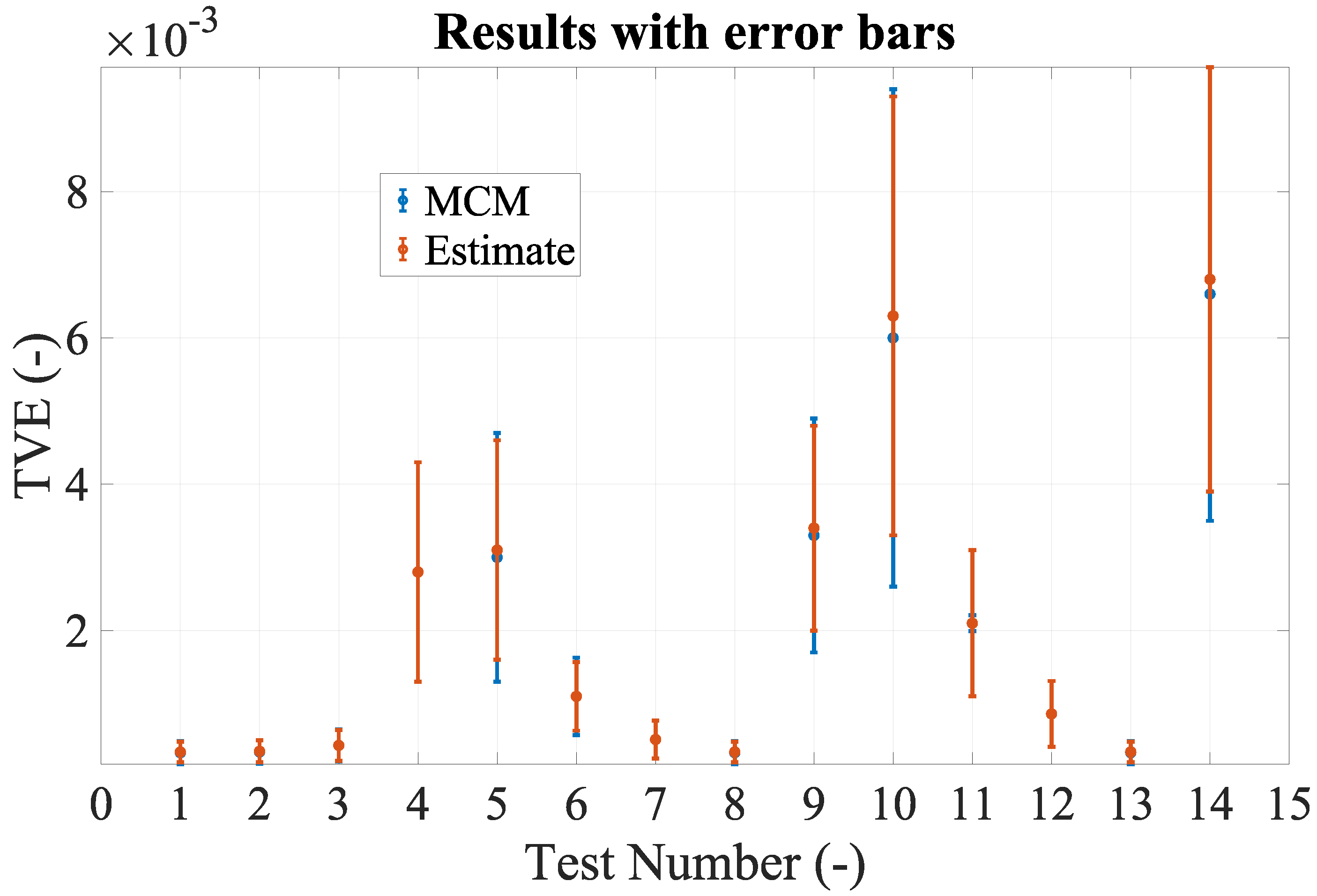
4.2. Results

Table 3. List of the results from the MCM testing.

Test	${\mathit{\mu }}_{TVE}$(−)	${\mathit{\sigma }}_{TVE}$(−)	${\widehat{\mathit{\mu }}}_{TVE}$(−)	${\widehat{\mathit{\sigma }}}_{TVE}$(−)
# 1	$3.3\times {10}^{-4}$	$1.6\times {10}^{-4}$	$3.4\times {10}^{-4}$	$1.4\times {10}^{-4}$
# 2	$3.4\times {10}^{-4}$	$1.6\times {10}^{-4}$	$3.5\times {10}^{-4}$	$1.5\times {10}^{-4}$
# 3	$4.3\times {10}^{-4}$	$2.2\times {10}^{-4}$	$4.3\times {10}^{-4}$	$2.1\times {10}^{-4}$
# 4	$2.8\times {10}^{-3}$	$1.5\times {10}^{-3}$	$2.8\times {10}^{-3}$	$1.5\times {10}^{-3}$
# 5	$3.0\times {10}^{-3}$	$1.7\times {10}^{-3}$	$3.1\times {10}^{-3}$	$1.5\times {10}^{-3}$
# 6	$1.1\times {10}^{-3}$	$5.3\times {10}^{-4}$	$1.1\times {10}^{-3}$	$4.7\times {10}^{-4}$
# 7	$5.1\times {10}^{-4}$	$2.6\times {10}^{-4}$	$5.1\times {10}^{-4}$	$2.6\times {10}^{-4}$
# 8	$3.3\times {10}^{-4}$	$1.6\times {10}^{-4}$	$3.4\times {10}^{-4}$	$1.4\times {10}^{-4}$
# 9	$3.3\times {10}^{-3}$	$1.6\times {10}^{-3}$	$3.4\times {10}^{-3}$	$1.4\times {10}^{-3}$
# 10	$6.0\times {10}^{-3}$	$3.4\times {10}^{-3}$	$6.3\times {10}^{-3}$	$3.0\times {10}^{-3}$
# 11	$2.1\times {10}^{-3}$	$1.1\times {10}^{-3}$	$2.1\times {10}^{-3}$	$1.0\times {10}^{-3}$
# 12	$8.6\times {10}^{-4}$	$4.5\times {10}^{-4}$	$8.6\times {10}^{-4}$	$4.5\times {10}^{-4}$
# 13	$3.3\times {10}^{-4}$	$1.6\times {10}^{-4}$	$3.4\times {10}^{-4}$	$1.4\times {10}^{-4}$
# 14	$6.6\times {10}^{-3}$	$3.1\times {10}^{-3}$	$6.8\times {10}^{-3}$	$2.9\times {10}^{-3}$

# is used to numerate the tests.

lists the results from the 14 tests performed by using the MCM. The table contains (i) the test number, (ii) the mean value and standard deviation obtained with the Matlab tools, ${\mu }_{\mathrm{TVE}}$ and ${\sigma }_{\mathrm{TVE}}$, respectively, and (iii) the mean value and standard deviation obtained with the developed expressions (54) and (55), ${\widehat{\mu }}_{\mathrm{TVE}}$ and ${\widehat{\sigma }}_{\mathrm{TVE}}$, respectively. Both standard deviations values have been written with two significant digits for the sake of comparison. With the same logic, and for increasing the readability, both mean values have been written with two significant digits. The choice of presenting the standard deviation in place of the variance is due to its higher significance in the confidence interval computation.

To increase the readability and comprehension of the results, they have been graphed with their error bar in Figure 3.

Starting from an overall look at the results, it is possible to confirm the efficacy and accuracy of the obtained expressions.

In detail, the tests vs phasor amplitude (#1 to #4) provide accurate results for both the estimates of mean and standard variation. A slight variation of the standard deviation ($0.2\times {10}^{-4}$), compared to the reference, can be noted for high values of the phasor $X$. This is due to its weight in all the expressions that led to (54) and (55) and to the Nakagami distribution, as explained in the following.

Analyzing tests #5 to #14, specific comments arise. First, in all tests the mean value is accurately estimated. Second, the error introduced by the delay and the gain are the most significant among all contributes. This is verified looking at tests #6, #10, and #11, in which the errors are 10, 10, and 20 times higher, respectively, than those selected as reference in test #1.

Third, the nonlinearity and noise errors are almost negligible in the TVE computation. This is highlighted from the results of tests #12 and #13 in which $L$ and $R$ are 20 times higher than the starting values but the TVE is comparable to it.

Finally, a potential reason for the found slight discrepancies in the standard deviation is the following. The numerator of (15) consists of the sum of 12 terms. Therefore, according to the central limit theorem, the distribution of the sum should tend to a normal distribution. However, it has been verified that it is not normally distributed, but it is something in-between a normal and a chi-square distribution. Hence, it is not a proper gamma distribution as required by the Nakagami distribution.

Overall, it can be concluded that:

• The obtained expressions to estimate the mean value and variance of the TVE have been confirmed to be applicable and effective in all the realistic conditions tested.
• The phase delay and the gain error are the most critical sources of error that increase the TVE. Therefore, when the ADC of a PMU must be selected, those two values should be as low as possible.
• Due to its expression, the TVE always has a mean value different from zero and positive in all nonideal conditions (hence, in all practical applications). Furthermore, the TVE distribution is not normal (and, in particular, it lays in-between a normal and a chi-square distribution), hence the information of the variance should be completed with the desired confidence interval. To this purpose, the cumulative distribution function of the Nakagami distribution must be used:

  $$F\left(x\right)=\frac{\gamma \left(m,\frac{m}{\mathsf{\Omega }}{x}^2\right)}{\mathsf{\Gamma }\left(m\right)}$$

  (55)

  where $\gamma ()$ is the lower incomplete gamma function.

5. Conclusions

The concept of achieving very accurate measurements can be extended to those parameters computed starting from such measurements. Therefore, this paper aimed at associating a confidence interval to the parameter used to assess the performance of a PMU; the TVE. To this purpose, the mathematic steps to obtain the closed-form expressions for the mean value and variance of TVE were described and then assessed by means of the MCM. The results from the realistic tests confirmed the validity and effectiveness of the developed expressions. Furthermore, such results aim at (i) highlighting which are the main sources that contribute to the TVE uncertainty (hence on the PMU uncertainty); (ii) providing to the manufacturer a simple tool to quantify the intrinsic uncertainty of his products and (iii) consequently the user will be given more details on the accuracy performance of the purchased PMU.

Another way of highlighting the findings of the work is to demonstrate the implications. In fact, the method that leads to find the expressions of mean and variance of the TVE can be customized according to the available information of the user. For example, the input parameters can be known as having specific probability distributions or values. In addition, the method can be replicated (not always) for other accuracy parameters as well. Overall, the study conclusions vary depending on the performed measurements and the parameters computed in the field.