A Data-Trait-Driven Rolling Decomposition-Ensemble Model for Gasoline Consumption Forecasting

Abstract

In order to predict the gasoline consumption in China, this paper propose a novel data-trait-driven rolling decomposition-ensemble model. This model consists of five steps: the data trait test, data decomposition, component trait analysis, component prediction and ensemble output. In the data trait test and component trait analysis, the original time series and each decomposed component are thoroughly analyzed to explore hidden data traits. According to these results, decomposition models and prediction models are selected to complete the original time series data decomposition and decomposed component prediction. In the ensemble output, the ensemble method corresponding to the decomposition method is used for final aggregation. In particular, this methodology introduces the rolling mechanism to solve the misuse of future information problem. In order to verify the effectiveness of the model, the quarterly gasoline consumption data from four provinces in China are used. The experimental results show that the proposed model is significantly better than the single prediction models and decomposition-ensemble models without the rolling mechanism. It can be seen that the decomposition-ensemble model with data-trait-driven modeling ideas and rolling decomposition and prediction mechanism possesses the superiority and robustness in terms of the evaluation criteria of horizontal and directional prediction.

1. Introduction

With the development of the economy and people’s living standards [1], car ownership has been increasing substantially [2]. As the main energy product of the transportation industry [3], gasoline also shows a trend of gradual increase. According to the related data from the National Bureau of Statistics of China, the number of private cars in China in 2018 was 205.74 million, a year-on-year increase of 11.13%. At the same time, China’s gasoline consumption in 2018 was 130.55 million tons with a year-on-year increase of 5.14%. It can be seen that the gasoline demand will continue to grow rapidly in the future; hence, effective forecasting of gasoline consumption can provide important measurement standards for the country, related industries, sales companies and individuals, which is of great significance.

For gasoline consumption forecasting, there have been many studies in the past few decades. According to the current research, there are four kinds of gasoline consumption forecasting models. They are the traditional statistical model, the artificial intelligence (AI) model, the hybrid model and the ensemble model.

In the traditional statistical model, it mainly includes the autoregressive integrated moving average model (ARIMA) [4,5], random walk (RW) model [6], grey forecast model [7], error correction model (ECM), Bayesian model average (BMA) [8], the panel data regression [9], and so on. The above models are often used to predict time series. For example, Bhutto et al. [10] used ARIMA to predict the gasoline consumption in the transportation sector. The empirical results showed the high prediction accuracy. Chen et al. [11] used the grey wave forecasting model for multi-step-ahead crude oil price forecasting. The empirical results showed that grey wave forecasting model had superior performance for multi-step-ahead crude oil price forecasting. Kapoguzov et al. [12] used a Bayesian approach to forecast the gasoline volume and price till 2026. Although this kind of model performed well in forecasting, it still has problems in analyzing complex and non-linear gasoline consumption data. Therefore, AI models were subsequently proposed for time series forecasting.

In the second category, AI methods mainly include heuristics, metaheuristics, and nature-inspired algorithms, etc. These methods are applied in many different domains, such as online learning [13], scheduling [14], medicine [15], multi-objective optimization, vehicle routing, and data classification, etc. Additionally, many AI models, such as back propagation neural network (BPNN) [16,17], random vector functional link (RVFL) [18], support vector regression (SVR) [19,20], extreme learning machine (ELM) [21], and wavelet neural network (WNN) [22], are widely used for energy forecasting. For example, Kazemi et al. [23] presented a hierarchical artificial neural network (ANN) method, which was based on supervised multilayer perceptron (MLP). Then the backpropagation (BP) algorithm was used for training to predict gasoline demand. The empirical results illustrated the prediction capability. Xie et al. [24] proposed a new model to predict crude oil price, which is based on support vector machine (SVM). The results showed that SVM was a good model to predict the crude oil price. Kulkarni et al. [25] proposed a model to forecast crude oil spot price direction in the short-term, which is based on the multilayer feedforward neural network (FNN). The results proved the forecasting effectiveness of the proposed model. Although the AI models can solve the nonlinear problems that traditional statistical models fail to solve, the AI models sometimes have the problem of overfitting, local optimization and parameter sensitivity. Therefore, hybrid models and ensemble models are adopted for these issues.

In the third category, different single prediction methods are used to formulate the hybrid model. The hybrid model includes the combination of different econometric models [26], the combination of AI models and econometric models [27,28], and the combination of different AI models [29,30]. For example, Xu et al. [31] presented an integrated model based on pattern modeling, recognition system (PMRS), error correction model (ECM) and artificial neural network (ANN) to forecast crude oil prices. Babazadeh et al. [32] presented a hybrid model for gasoline consumption forecasting, which was based on ANN and ARIMA approach. The results showed the prediction capability of the hybrid ARIMA-ANN method. Li et al. [33] integrated a firefly algorithm (FA) with least squares support vector regression (LSSVR) for forecasting. The results showed that the proposed model had better prediction performance than other benchmark models. Accordingly, these existing studies showed that the hybrid models can improve the prediction accuracy effectively.

In the fourth category, because the ensemble model is the integrated prediction of multiple same-type models, it can solve the issues that caused by the single model. It mainly include Bagging [34,35], Boosting [36], AdaBoost [37], and XGBoost [38,39], etc. At present, the ensemble model is widely used in various domains. For example, ensemble methods were employed for the classification problem for power systems security assessment in [40]. The decision tree based ensemble method was proposed for the case of concept drift in datasets in [41]. Besides, the ensemble model is also adopted to predict the energy. Specifically, Zhao et al. [42] utilized stacked denoising autoencoders (SDAE) and bootstrap aggregation (bagging) to deal with the problem of crude oil forecasting. The approach showed superior prediction ability in three statistical tests. Qu et al. [43] used empirical mode decomposition (EMD) and BPNN adaptive boosting (BP_AdaBoost) to model the oil price. The empirical results showed that it effectively improved the short-term price forecasting accuracy compared with other listed models. Su et al. [44] proposed the least squares regression boosting (LSBoost) algorithm to forecast the natural gas spot prices. The empirical results revealed that this method had a superior prediction performance.

Next, Yu et al. [45] first proposed the decomposition-ensemble model, which belongs to a new type of the ensemble model. The decomposition-ensemble learning paradigm is based on the idea of “divide-and-conquer”. First, multi-scale decomposition of the original data is performed. Then, each component is predicted separately. Finally, the prediction results of these components are aggregated to output the final prediction result. Decomposition-ensemble models can reduce the complexity of modeling and improve the prediction performance, especially for nonlinear time series data [46]. For example, He et al. [47] proposed a wavelet decomposed ensemble model to forecast the oil price. The empirical results showed that the prediction performance of the proposed algorithm was better than that of the benchmark models. Tang et al. [48] proposed a CEEMD-EELM model, i.e., complementary ensemble empirical mode decomposition (CEEMD) and extended extreme learning machine (EELM) to predict the oil price. The results revealed that the proposed model had better performance than all listed benchmark models. Tang et al. [49] proposed randomized-algorithm-based decomposition-ensemble learning models for forecasting. The proposed models were proved to be efficient and fast. Although the “divide-and-conquer” strategy was used by the decomposition-ensemble model to reduce the complexity of modeling and improve prediction performance, the data traits of the original data didn’t be considered by the many existing models. Therefore, in response to this problem, data-trait-driven modeling idea was proposed by some scholars to select suitable models in terms of the traits hidden in the data [50].

In the novel “data-trait-driven modeling” method, data analysis and forecast modeling, are mainly involved [48]. Starting from the traits of the data, the model that matches its traits can be built, so as to better analyze and improve the prediction accuracy. In fact, “data-trait-driven modeling” has been adopted to build some effective predictive learning paradigms and improve prediction performance. For example, Wang et al. [51] proposed a seasonal decomposition (SD)-based least squares support vector regression (LSSVR) ensemble learning paradigm for hydropower consumption forecasting. The results showed that the proposed model was a superior approach for seasonal time series prediction. Tang et al. [52] proposed a mode-trait-based decomposition ensemble model to predict nuclear energy consumption. The results demonstrated that the data-trait-driven model strikingly improved prediction performance. Yu et al. [53] proposed a methodology combined “divide and conquer” and “data-trait-driven modeling” for crude oil price forecasting. The results indicated the effectiveness of the proposed model.

According to the existing studies, it is easy to find that although the decomposition-ensemble methods based on data traits have made great progress in prediction, some problems with these models are still existed. For example, Wang et al. [51] only considered the seasonal trait of original series in hydropower data, but did not consider the component traits after decomposition. They directly used LSSVR model for component prediction without reasons. Furthermore, in the existing decomposition-ensemble forecasting studies, there was an improper information use case. However, the testing dataset data is unknown in actual problems. Therefore, decomposing the testing dataset is equivalent to using future information to make predictions, which leads to the errors of prediction results.

Accordingly, for the purpose of solving the above problems, this paper not only considers the data traits of the original time series data and decomposed component data, but also decomposes the training data only instead of the overall data. This is the difference between the existing literature and this paper. In order to further improve the forecasting performance, the rolling decomposition and prediction mechanism are introduced into the data-trait-driven decomposition ensemble model for gasoline consumption forecasting. Additionally, the prediction performance of the proposed data-trait-driven rolling decomposition-ensemble model is compared with some typical benchmark models.

The main purpose of this paper is to propose a data-trait-driven rolling decomposition-ensemble learning model to predict gasoline consumption. In the proposed model, at first, the original data of the gasoline consumption is used to test their main data trait to determine the decomposition method. Then the original data is decomposed into multiple components. Next, component trait analysis is performed on each mode component to determine the component prediction method. Subsequently, each mode component is forecasted separately in terms of their own traits. Finally, the prediction results of each component are integrated to obtain the final prediction result. In order to verify the effectiveness of the model, the quarterly gasoline consumption data from four provinces in China are used. In addition, to verify the robustness of the proposed model, Diebold-Mariano (DM) test is adopted. The rest of the paper is organized as follows. The methodology formulation is described in Section 2. The empirical results are introduced in Section 3. The conclusions and future directions are elaborated in Section 4.

2. Methodology Formulation

The formulation process of the proposed model is introduced in this section. Specifically, the general framework of the proposed model is given in Section 2.1. The related technologies of the data-trait-driven data decomposition, data-trait-driven component prediction and data-trait-driven ensemble output are introduced in Section 2.2, Section 2.3 and Section 2.4. The rolling decomposition and prediction mechanism is described in Section 2.5.

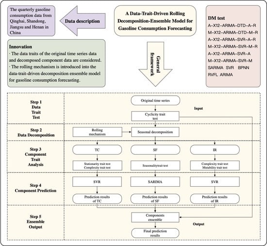
2.1. General Frameworks of the Proposed Methodology

Gasoline consumption data fluctuates widely and irregularly, which brings about great challenges to forecasting. For the purpose of improving the prediction performance, a data-trait-driven rolling decomposition-ensemble learning methodology is proposed. Particularly, the idea of “data-trait-driven modeling”, “decomposition and ensemble” and the rolling mechanism are adopted. In order to proceed from the traits of the data itself and explore the hidden data traits, the data traits of the original data and decomposed component data are analyzed. Not only that, in order to fully use the known knowledge in the training dataset, the rolling decomposition and ensemble mechanism is adopted into the general framework. The framework of the data-trait-driven rolling decomposition-ensemble learning paradigm can be illustrated in Figure 1.

As can be seen from Figure 1, the proposed data-trait-driven rolling decomposition-ensemble learning paradigm consists of five steps, those are data trait test, data decomposition, component trait analysis, component prediction and ensemble output, which are elaborated below.

Step 1: Data Trait Test

Due to the effect of economic, social environment and other factors, the quarterly gasoline consumption data has relatively regular cyclicity fluctuations every year. Thus, the cyclicity trait of the original time series data is tested. Accordingly, the autocorrelation analysis is used as the main method for the cyclicity trait test [54] in this paper. In terms of the cyclicity trait, seasonal decomposition is adopted as the decomposition method for original gasoline consumption data, as it can remove the influence of seasonal fluctuations, as shown in Step 1 of Figure 1. The steps of the data trait test and related technologies will be introduced in detail in Section 2.2.

Step 2: Data Decomposition

In the second step, in order to reduce the modeling difficulty of the complex system, the original data is decomposed at multiple components with different scales. According to the result of Step 1, the seasonal decomposition is selected as the decomposition method for original time series data. Accordingly, two decomposition forms are adopted respectively, namely additive decomposition and multiplicative decomposition. Additionally, the original time series data with the cyclicity trait is decomposed into three components with different meanings and scales: trend cycle (TC), seasonal factor (SF), and irregular component (IR). During the decomposition process, the gasoline consumption data is decomposed through the rolling decomposition and prediction mechanism. In each decomposition, new known training data is added until all the testing data are predicted. Therefore, the existing knowledge can be fully used in such process, which lays a solid foundation for the subsequent prediction. The related technologies of data decomposition are described in detail in Section 2.2.

Step 3: Component Trait Analysis

In the third step, three main components are decomposed in Step 2: TC, SF, and IR, are respectively analyzed for data trait exploration. For different components, different component trait test methods are used. Firstly, in the data trait analysis of TC, the Augmented Dickey–Fuller (ADF) test is used to test the stationary trait of TC. If TC is non-stationary, the permutation entropy (PE) test is adopted to estimate the complexity trait of TC. According to the above tests, the data traits of TC component can be judged and the corresponding prediction model can be selected. Secondly, in the data trait analysis of SF, autocorrelation analysis is used to test the seasonality trait of SF. Then the prediction model of SF can be selected according to seasonality trait of SF. Thirdly, in the data trait analysis of IR, the complexity trait is tested using permutation entropy (PE) test. If IR has complexity trait, the mutability trait is tested. In the mutability trait test, first perform the iterative cumulative sum of squares (ICSS) test to find the suspect points of IR, and then Chow test is used to test the mutability trait of suspect points. The steps of component trait analysis and related techniques will be introduced in Section 2.3.

Step 4: Component Prediction

In order to obtain the prediction results of the components, the corresponding prediction model is chosen to predict each component separately according to their data traits obtained in the Step 3. Because SVR can alleviate overfitting and local minimum problems, it has superior prediction performance. Therefore, an adaptive, stable and flexible SVR can be used as a prediction model for components with complexity trait or mutability trait. In addition, because SARIMA is a model with seasonal difference operators, it can be used as the prediction model for data with seasonality trait. Then each component is predicted by corresponding prediction models to get component prediction results. The steps of component prediction and related techniques will be described in detail in Section 2.3.

Step 5: Ensemble Output

In the Step 5, according to the decomposition-ensemble principle, the component prediction results are fused, as shown in Step 5 of Figure 1. The component forecasting results are fused to output the final prediction result using the selected ensemble method. Specifically, according to the data trait analysis in the Step 1 and the selection of the decomposition method in the Step 2, the corresponding ensemble model will be selected to fuse the component prediction results. The steps of ensemble output and related techniques will be described in Section 2.4.

2.2. Data-Trait-Driven Data Decomposition

In this section, the cyclicity trait test in Step 1 of Figure 1 and the seasonal decomposition in Step 2 of Figure 1 are introduced. For this purpose, autocorrelation analysis is used as a method of cyclicity trait test, which is introduced in Section 2.2.1. Meantime, X-12-ARIMA is used as a seasonal decomposition method to decompose data with the cyclicity trait, which is introduced in Section 2.2.2.

2.2.1. Cyclicity Trait Test

The cyclicity trait mainly refers to the fact that the data repeats the previous fluctuations at a fairly regular time interval, often accompanied by peaks and valleys. These fluctuations are the important factor hidden within the data, revealing the main laws of time series data. Therefore, the cyclicity trait reflects the unique impact factors and potential laws of the time series data, which is one of the most important data traits [55]. For the quarterly gasoline consumption data, due to the economic and social environment and other factors, it has relatively regular cyclicity fluctuations every year. Therefore, the cyclicity trait test is conducted on the gasoline consumption time series data, as shown in Step 1 of Figure 1.

As autocorrelation (AC) analysis measures the correlation between two points at a given interval in the time series, it is helpful to determine the cycle period scale in the data. For the quarterly gasoline consumption data, this method can determine whether there is a cyclicity pattern in the observed time series data. Therefore, in this paper, the autocorrelation analysis is performed as the method of the cyclicity trait test. The specific processes can be referred to in the literature [56] for more details.

2.2.2. Seasonal Decomposition (SD)

This section describes the decomposition method adopted in Step 2 of Figure 1. For the gasoline consumption data with the cyclicity trait, it has periodic changes caused by the influence of seasonal components, which is called seasonal fluctuation in the economic analysis. Because the seasonal decomposition (SD) method can remove cyclicity elements from the original time series with the cyclicity trait, so as to remove the influence of seasonal fluctuations. Therefore, the seasonal decomposition (SD) method is used for the decomposition method in this paper.

In the existing SD method, X-12-ARIMA can extract seasonal patterns hidden in time series data. Not only that, X-12-ARIMA is the seasonal adjustment program of the Census Bureau [57]. Therefore, this paper will adopt X-12-ARIMA as the SD method. Accordingly, the time series X_t is decomposed by the X-12-ARIMA method into three components, i.e., the trend cycle TC_t, the seasonal factor SF_t and the irregular component IR_t. The X-12-ARIMA method has a variety of forms to combine these components into original data. Generally, the forms mainly include the additive form of Equation (1) and the multiplicative form of Equation (2):

$$X_t=T{C}_t+S{F}_t+I{R}_t$$

(1)

$$X_t=T{C}_t\times S{F}_t\times I{R}_t$$

(2)

As for which form of X-12-ARIMA is selected, it depends on different gasoline consumption data. The specific form will be selected from the experimental results.

2.3. Data-Trait-Driven Component Prediction

In this section, the component trait analysis in Step 3 of Figure 1 and the component prediction in Step 4 of Figure 1 are introduced in this section. Specifically, this section illustrates the main methods of component trait analysis, including the complexity trait test and the mutability trait test. In addition, the details of two important prediction models, i.e., seasonal auto regressive integrated moving average (SARIMA) and support vector regression (SVR) can be referred to in the given specific literature.

For the three components decomposed in Step 2, their data traits will be analyzed separately in order to find the suitable prediction model corresponding to each decomposed component. As introduced in Section 2.2.2, the original data is decomposed by X-12-ARIMA into the trend cycle (TC), the seasonal factor (SF) and the irregular component (IR). For these components, different data trait test methods are used in terms of their traits.

Firstly, the trend cycle (TC) term represents the long-term trend of the original time series. Therefore, for the time series with long-term trends, ADF test is first used to test its stationarity. If it is stationary, traditional statistical and econometric model is suitable for prediction in order to save time. If it is non-stationary, its complexity trait need to be further tested to determine whether there are many internal disorder components in its dynamic system. Thus, the permutation entropy (PE) first proposed by Bandt and Pompe [48] can be used to test whether it has complexity trait. According to the result of PE test, the prediction model can be determined to predict the TC.

As one of the complexity trait test methods, PE estimates the complexity of data dynamics by mapping time series into symbol sequences. When the PE value is less than the given threshold h, the component appears low complexity. Likewise, the component with PE value above h has high complexity. In this paper, the threshold h is set to 0.5. Compared with other methods (such as sample entropy), it has the advantages of simplicity, speed and stationary. In addition, even for complex data with a lot of noise, the PE can perform well [58]. Specific steps can be referred to in the literature [59] for more details.

Secondly, the seasonal factor (SF) refers to the cyclical changes that occur repeatedly every four quarters, resulting in a cyclical effect. Seasonal change is a self-circulation in a fixed interval. Therefore, the seasonal trait needs to be tested. Accordingly, the autocorrelation analysis can be used to test whether the time series has seasonality trait. If it has seasonal trait, a model that adapts to the data with seasonal trait can be selected to predict the SF.

Thirdly, the irregular component (IR) is also called random factor. Its changes have no rules to follow, usually caused by accidental events. Therefore, for this more complex sequence, the permutation entropy (PE) can be used to test whether it has complexity trait. If it has, the iterative cumulative sum of squares (ICSS) can be further used to find whether it has the suspect breaking points [60], and the Chow test at the suspect breaking points can be used to test its mutability trait [61].

In summary, for decomposed three components, the stationarity trait and complexity trait are tested for the trend cycle (TC), the seasonal trait is tested for the seasonal factor (SF), and the complexity trait and mutability trait are tested for the irregular component (IR). In terms of these different component traits, different forecasting models are selected for prediction purpose.

In the component prediction, because the seasonal auto-regressive integrated moving average (SARIMA) model is an ARIMA-based econometrical method, which is often used to deal with time series data containing periodic fluctuations [62]. Therefore, the SARIMA model can be used to predict the data with seasonality trait. Moreover, based on Vladimir Vapnik’s concept of support vectors [63,64], support vector regression (SVR) has been proposed. As SVR is adaptive, stable and flexible and it has the global approximation capability for data scarcity issue, it can be used as the prediction model for the data with complexity trait and mutability trait.

2.4. Data-Trait-Driven Ensemble Output

In this section, the ensemble method of Step 5 in Figure 1 is introduced. In this step, the ensemble method integrates the forecasting results of TC, SF, IR to obtain the final forecasting result. Corresponding to the two forms of X-12-ARIMA decomposition model in Section 2.2.2, which are shown in Equations (1) and (2), the ensemble method also has two forms. Accordingly, the specific expressions are shown in Equations (3) and (4) below.

$$\widehat{X_t}=\widehat{T{C}_t}+\widehat{SF}+\widehat{I{R}_t}$$

(3)

$$\widehat{X_t}=\widehat{T{C}_t}\times \widehat{SF}\times \widehat{I{R}_t}$$

(4)

where $\widehat{X_t}$ is the forecasting result as shown in Figure 1. $\widehat{T{C}_t}$, $\widehat{SF}$, $\widehat{I{R}_t}$ is the forecasting result of the component $T{C}_t$, $S{F}_t$, $I{R}_t$ respectively. As for which specific form of ensemble method is selected, it depends on the form of the decomposition method.

2.5. Rolling Decomposition and Forecasting Mechanism

In the existing studies, the training dataset and testing dataset in the decomposition ensemble model are decomposed at the same time. However, in actual problems, the testing dataset represents future information and cannot be used for the training process. Therefore, if the rolling decomposition and prediction mechanism is introduced into the decomposition ensemble model, the accuracy of the prediction results will be ensured.

Considering that the forecasting problem is carried out under the premise that the testing data is unknown, when using the decomposition model, the decomposed data should always be the existing data. In the rolling mechanism, one testing data point is forecasted at a time. When predicting the next data point, the current data point is considered to be known. This method can make full use of existing data to ensure the maximum knowledge learning. More details about rolling decomposition and prediction mechanism can refer to the Yu et al. [65].

3. Empirical Analysis

To verify the effectiveness of the proposed model, quarterly gasoline consumption data from Qinghai Province, Shandong Province, Jiangsu Province, and Henan Province in China are used as sample data. Accordingly the experimental design is introduced in Section 3.1, the experimental results are analyzed in Section 3.2, the further discussions are shown in Section 3.3, and the main findings are summarized in Section 3.4.

3.1. Experimental Design

In this paper, the quarterly gasoline consumption data of Qinghai Province, Shandong Province, Jiangsu Province, and Henan Province are used. Moreover, the data is originated from the National Bureau of Statistics of China. The time of each sample data is from the first quarter of 2010 to the fourth quarter of 2018, and there are a total of 36 observations in each province, as shown in Figure 2, Figure 3, Figure 4, Figure 4, Figure 5. In the gasoline consumption data of each province, the ratio of training dataset to testing dataset is 28:8.

In order to compare the forecasting performance of different models, horizontal prediction accuracy and directional prediction accuracy are selected as the evaluation criteria for forecasting performance. Accordingly, mean absolute percentage error (MAPE) and root mean squared error (RMSE) are used as the horizontal prediction accuracy. Meantime, the directional statistics ($D_{stat}$) is selected as the directional prediction accuracy. MAPE and RMSE can be represented by:

$$MAPE=\frac{1}{N}{\displaystyle \sum }_{t=1}^N\left|\frac{x_t-{\widehat{x}}_t}{x_t}\right|$$

(5)

$$RMSE=\sqrt{\frac{1}{N}{\displaystyle \sum }_{t=1}^N{\left(\widehat{x_t}-x_t\right)}^2}$$

(6)

where $x_t$ is obserbed value, ${\widehat{x}}_t$ is forecasting value, N is the length of testing dataset. The smaller the values of MAPE and RMSE, the better the horizontal prediction accuracy.

$D_{stat}$ is expressed by:

$$D_{stat}=\frac{1}{N}{\displaystyle \sum }_{t=1}^N{a}_t\times 100\%$$

(7)

where $a_t=1 if \left(x_{t+1}-x_t\right)\left({\widehat{x}}_{t+1}-x_t\right)\ge 0$, and $a_t=0$ otherwise. The larger the values of $D_{stat}$, the better the directional prediction accuracy.

Moreover, in order to prove the superiority of the proposed model in this paper, we also used some single models to predict gasoline consumption. Specifically, as a representative of the traditional statistical model, ARIMA was used. As a single model with seasonal factors, SARIMA was used. As a representative of artificial intelligence models, SVR, BPNN and RVFL were used.

In addition, in order to select the decomposition model suitable for each province, the SVR is used as a prediction model to build the decomposition-ensemble model due to its good prediction performance. Based on the above descriptions, four decomposition-ensemble models were constructed. They are A-X12-ARIMA-SVR-A, M-X12-ARIMA-SVR-M, A-X12-ARIMA-SVR-A-R, M-X12-ARIMA-SVR-M-R. Besides, there are models proposed in this paper, namely A-X12-ARIMA-DTD-A-R, M-X12-ARIMA-DTD-M-R. In these models, the first ‘A’ represents additive decomposition, and the second ‘A’ represents additive ensemble. The first ‘M’ represents multiplicative decomposition, and the second ‘M’ represents multiplicative ensemble. ‘R’ means it has the rolling decomposition and prediction mechanism. ‘DTD’ represents data-trait-driven modeling.

3.2. Experimental Results Analysis

This section mainly analyzes the empirical results. Specifically, Section 3.2.1 analyzes the results of the original time series data trait test. Section 3.2.2 analyzes the different decomposition forms of the four provinces in order to determine the decomposition model. Section 3.2.3 illustrates the analysis results of the different traits of each component. Section 3.2.4 analyzes the prediction performance of different models and verifies the effectiveness of the proposed model.

3.2.1. Data Trait Test

In this section, the cyclicity trait of the original time series data was tested. Accordingly, autocorrelation (AC) analysis was performed on the quarterly gasoline consumption data to determine whether there is a cyclicity pattern in the observed time series data. The cyclicity trait test results of the 4 time series data are shown in

Table 1. Cyclicity test results of original time series data.

Time Series	Lag Period	Correlation Coefficient	Statistics	Prob.	Time Series
Qinghai	4	0.738	70.728	0.000	Qinghai
Henan	4	0.812	39.229	0.000	Henan
Shandong	4	0.735	68.684	0.000	Shandong
Jiangsu	4	0.736	61.159	0.000	Jiangsu

.

As shown in Table 1, when the lag period of four provinces is four quarters, the correlation coefficient of the time series data is the largest. The test results show that the four time series data in Table 1 have a cyclicity trait with a period of one year (four quarters).

3.2.2. Data Decomposition Analysis

As introduced in Section 2.2.2, X-12-ARIMA has two forms of decomposition. Therefore, this section uses the four decomposition-ensemble models mentioned in Section 3.1 to find the decomposition method suitable for different provinces. These models are A-X12-ARIMA-SVR-A, M-X12-ARIMA-SVR-M, A-X12-ARIMA-SVR-A-R, M-X12-ARIMA-SVR-M-R. Moreover, in terms of the evaluation criteria of horizontal and directional prediction,

Table 2. The prediction performance of gasoline consumption in Qinghai.

Forecasting Models	MAPE	RMSE	Dstat
A-X12-ARIMA-SVR-A	0.23269	5.48188	0.42857
M-X12-ARIMA-SVR-M	0.30811	6.72903	0.42857
A-X12-ARIMA-SVR-A-R	0.05063	1.20584	1.00000
M-X12-ARIMA-SVR-M-R	0.05323	1.30603	1.00000

,

Table 3. The prediction performance of gasoline consumption in Shandong.

Forecasting Models	MAPE	RMSE	Dstat
A-X12-ARIMA-SVR-A	0.01350	4.32930	0.57143
M-X12-ARIMA-SVR-M	0.01393	4.40868	0.42857
A-X12-ARIMA-SVR-A-R	0.00832	2.64259	1.00000
M-X12-ARIMA-SVR-M-R	0.00873	2.73930	1.00000

,

Table 4. The prediction performance of gasoline consumption in Henan.

Forecasting Models	MAPE	RMSE	Dstat
A-X12-ARIMA-SVR-A	0.48476	138.39043	0.71429
M-X12-ARIMA-SVR-M	0.48202	150.08664	0.57143
A-X12-ARIMA-SVR-A-R	0.17552	34.80237	1.00000
M-X12-ARIMA-SVR-M-R	0.07182	21.38547	1.00000

and

Table 5. The prediction performance of gasoline consumption in Jiangsu.

Forecasting Models	MAPE	RMSE	Dstat
A-X12-ARIMA-SVR-A	0.15223	44.59431	0.42857
M-X12-ARIMA-SVR-M	0.15893	47.27334	0.42857
A-X12-ARIMA-SVR-A-R	0.08419	22.41964	0.85714
M-X12-ARIMA-SVR-M-R	0.07750	20.53079	1.00000

show the prediction performance of these four prediction models for Qinghai, Shandong, Henan, and Jiangsu respectively.

From the evaluation criteria of horizontal and directional prediction in Table 2, Table 3, Table 4, Table 5, two important results can be found below.

(1) Generally, the prediction performance of decomposition-ensemble model with rolling mechanism is better than that of decomposition-ensemble model without rolling mechanism for all four provinces. This implies that the introduction of the rolling decomposition and prediction mechanism is very effective in improving the prediction performance. This result is consistent with the previous finding in Yu et al. [65].

(2) For the decomposition forms, there are some distinct differences between the former two provinces (i.e., Qinghai and Shandong in Table 2 and Table 3) and the latter two ones (i.e., Henan and Jiangsu in Table 4 and Table 5). For the former two provinces, the prediction performance of additive decomposition is better than that of multiplicative decomposition, while the result is somewhat different for the latter two provinces. That is, the prediction performance of multiplicative decomposition is better than that of additive decomposition under the condition of rolling mechanism for the latter two provinces, indicating the effectiveness of rolling mechanism again. The possible reason leading to the differences is that the data of the former two provinces has less fluctuation than the latter two ones.

In summary, if the proposed decomposition-ensemble model does not apply the rolling mechanism, the additive decomposition is more suitable for gasoline consumption forecasting than the multiplicative decomposition. If the proposed decomposition-ensemble model adopts the rolling mechanism, the prediction performance of the additive decomposition is better than that of the multiplicative decomposition for the data with small fluctuation, while the multiplicative decomposition is better than the additive decomposition for the data with high volatility.

3.2.3. Component Trait Analysis

In this section, in order to find the suitable prediction model corresponding to each component, the data traits of these three components (i.e., TC, SF and IR) will be analyzed, as illustrated below.

The trend cycle (TC)

For the training dataset (i.e., the data from the first quarter of 2010 to the fourth quarter of 2016), TC terms of the four provincial administrative units are shown in Figure 6, Figure 7, Figure 8, Figure 9.

For TC terms, the ADF test is first used to test the stationarity trait. The corresponding results of ADF test are presented in

Table 6. Stationarity trait test results for TC.

	Qinghai	Shandong	Henan	Jiangsu
Prob.	0.2277	0.2597	0.9995	0.9217

.

It can be seen from Table 6 that the TC terms of these four provinces is non-stationary. Therefore, their complexity trait is tested. The results of permutation entropy (PE) test are given in

Table 7. Complexity trait test results for TC.

	Qinghai	Shandong	Henan	Jiangsu
PE values	0.0720	0.3694	0.0000	0.3636

.

In terms of the previous studies, the threshold h is set to 0.5. In Table 7, all the PE values of the TC terms in four provinces are lower than h and the PE value of Henan’s TC is even 0. Therefore, the TC terms decomposed by X-12-ARIMA in Qinghai, Shandong, and Jiangsu have low complexity and Henan does not have complexity trait.

In general, the TC term is used to find the long-term trend of the original time series data. After the permutation entropy test, it was found that the TC in Qinghai, Shandong, and Jiangsu was accompanied by lower complexity, and the TC in Henan had no complexity. As a whole, the trend of TC term rises steadily, as shown in Figure 3. Accordingly, the adaptive, stable and flexible SVR can be used as the prediction model of TC term.

The seasonal factor (SF)

For the training dataset (i.e., the data from the first quarter of 2010 to the fourth quarter of 2016), SF terms of the 4 provincial administrative units are shown in Figure 10, Figure 11, Figure 12 and Figure 13.

According to Section 2.3 the autocorrelation analysis is used to test whether it has seasonality trait.

Table 8. Seasonality trait test results for SF.

Time Series	Lag Period	Correlation Coefficient	Statistics	Prob.
Qinghai	2	−0.871	24.590	0.000
Henan	4	0.859	49.274	0.000
Shandong	4	0.803	32.427	0.000
Jiangsu	2	−0.929	27.877	0.000

shows the results of the seasonality trait test.

In Table 8, when the lag period in Qinghai and Jiangsu is 2 quarters, the correlation coefficient of the SF term is the largest. The results show that the SF terms in Qinghai and Jiangsu decomposed by X-12-ARIMA has seasonality trait with a period scale of 2 quarters. Similarly, the SF terms in Henan and Shandong decomposed by X-12-ARIMA has seasonality trait with a period scale of 4 quarters. Therefore, all the seasonal factors of these four provinces repeat the sequence with the different peaks and valleys respectively. As SARIMA is a single model with seasonal factors, it can model economic time series for any period. Therefore, SARIMA is selected as the prediction model of seasonal factor in this paper.

The irregular component (IR)

For the training dataset (i.e., the data from the first quarter of 2010 to the fourth quarter of 2016), IR terms of the 4 provincial administrative units are shown in Figure 14, Figure 15, Figure 16, Figure 17.

In this paper, the PE test is used as the method of complexity trait test. Accordingly the PE values of IR terms are listed in

Table 9. Complexity trait test results for IR.

	Qinghai	Shandong	Henan	Jiangsu
PE values	0.6035	0.5823	0.6276	0.6156

.

In Table 9, all the PE values of the IR in four provinces are higher than h (h = 0.5). Therefore, all the IR terms of these four provinces have complexity trait. For this reason, the iterative cumulative sum of squares (ICSS) is used to find the suspect points, and the Chow test is adopted to test mutability trait at the suspect points. The corresponding results of ICSS test and Chow test are listed in

Table 10. Mutability trait test results for IR.

Province	Suspect Points	ICSS Test	Chow Test	Mutability
Qinghai	2015Q2	2.546 (0.005)	2.788 (0.003)	√
Shandong	2012Q3	1.803 (0.036)	2.527 (0.006)	√
Henan	-	-	-	×
Jiangsu	-	-	-	×

.

It can be seen from Table 10 that the suspect points of the IR terms in Qinghai and Shandong are the second quarter of 2015 and the third quarter of 2012 in terms of ICSS test results. The further Chow test results show that the IR terms of Qinghai and Shandong have a mutability trait. In addition, the empirical test results show that the IR terms of Henan and Jiangsu do not have mutability trait.

In summary, all the IR terms of Qinghai, Shandong, Henan, and Jiangsu have complexity trait. In addition, the IR terms of Qinghai and Shandong have mutability trait. Therefore, an adaptive, stable and flexible SVR is selected as the prediction model for IR terms.

Based on the optimal decomposition method of each province drawn from the above conclusions, we can construct different models for 4 provinces in China.

(1) Overall, the X-12-ARIMA decomposition-ensemble model with the rolling mechanism is used by four provinces.

(2) X-12-ARIMA additive decomposition is adopted to decompose the data of Qinghai and Shandong, and X-12-ARIMA multiplicative decomposition is adopted in Henan and Jiangsu.

(3) Based on the analysis and description in this section, for the component prediction models in the four provinces, SVR model is selected for TC terms and IR terms forecasting and SARIMA model is used to predict SF terms.

(4) Corresponding to different forms of the X-12-ARIMA decomposition method, the additive ensemble is adopted in Qinghai and Shandong, and the multiplicative ensemble is adopted in Henan and Jiangsu.

From the above descriptions, this paper will use the A-X12-ARIMA-DTD-A-R model to predict gasoline consumption in Qinghai and Shandong, and use the M-X12-ARIMA-DTD-M-R model to predict gasoline consumption in Henan and Jiangsu. The corresponding prediction results and prediction performance analysis will be elaborated in Section 3.2.4.

3.2.4. Prediction Performance Analysis

This section mainly shows the prediction performance of 10 prediction models in 4 provinces in terms of the evaluation criteria of horizontal and directional prediction. These 10 models include ARIMA, BPNN, SVR, RVFL, SARIMA, A-X12-ARIMA-SVR-A, M-X12-ARIMA-SVR-M, A-X12-ARIMA-SVR-A-R, M-X12-ARIMA-SVR-M-R, and A(M)-X12-ARIMA-DTD-A(M)-R. Accordingly

Table 11. Performance comparison of different models in Qinghai.

Forecasting Models	MAPE	RMSE	Dstat
ARIMA	0.0931	1.9145	0.8571
BPNN	0.0538	1.2299	0.8571
SVR	0.1321	3.5025	0.5714
RVFL	0.2249	4.8609	0.8571
SARIMA	0.0714	1.8084	1.0000
A-X12-ARIMA-SVR-A	0.2327	5.4819	0.4286
M-X12-ARIMA-SVR-M	0.3081	6.7290	0.4286
A-X12-ARIMA-SVR-A-R	0.0506	1.2058	1.0000
M-X12-ARIMA-SVR-M-R	0.0532	1.3060	1.0000
A-X12-ARIMA-DTD-A-R	0.0461	1.1035	1.0000

,

Table 12. Performance comparison of different models in Shandong.

Forecasting Models	MAPE	RMSE	Dstat
ARIMA	0.0118	3.7188	0.5714
BPNN	0.0087	2.9310	0.7143
SVR	0.0083	3.0276	1.0000
RVFL	0.0260	9.6263	0.7143
SARIMA	0.0220	7.2544	0.5714
A-X12-ARIMA-SVR-A	0.0135	4.3293	0.5714
M-X12-ARIMA-SVR-M	0.0139	4.4087	0.4286
A-X12-ARIMA-SVR-A-R	0.0083	2.6426	1.0000
M-X12-ARIMA-SVR-M-R	0.0087	2.7393	1.0000
A-X12-ARIMA-DTD-A-R	0.0078	2.6302	1.0000

,

Table 13. Performance comparison of different models in Henan.

Forecasting Models	MAPE	RMSE	Dstat
ARIMA	0.1827	32.6324	1.0000
BPNN	0.1239	25.6547	1.0000
SVR	0.2470	60.3990	0.8571
RVFL	0.4914	125.4011	0.8571
SARIMA	0.1916	43.4215	1.0000
A-X12-ARIMA-SVR-A	0.4848	138.3904	0.7143
M-X12-ARIMA-SVR-M	0.4820	150.0866	0.5714
A-X12-ARIMA-SVR-A-R	0.1755	34.8024	1.0000
M-X12-ARIMA-SVR-M-R	0.0718	21.3855	1.0000
M-X12-ARIMA-DTD-M-R	0.0601	15.2771	1.0000

and

Table 14. Performance comparison of different models in Jiangsu.

Forecasting Models	MAPE	RMSE	Dstat
ARIMA	0.1602	46.3598	0.8571
BPNN	0.0969	32.4150	1.0000
SVR	0.1136	32.7750	0.4286
RVFL	0.4933	167.9224	0.7143
SARIMA	0.1109	32.5558	0.8571
A-X12-ARIMA-SVR-A	0.1522	44.5943	0.4286
M-X12-ARIMA-SVR-M	0.1589	47.2733	0.4286
A-X12-ARIMA-SVR-A-R	0.0842	22.4196	0.8571
M-X12-ARIMA-SVR-M-R	0.0775	20.5308	1.0000
M-X12-ARIMA-DTD-M-R	0.0621	16.9129	1.0000

show the prediction performance of these models for gasoline consumption in Qinghai, Shandong, Henan, and Jiangsu, respectively.

From the results shown in Table 11, Table 12, Table 13 and Table 14, five main findings can be summarized.

Firstly, in terms of three evaluation criteria, the data-trait-driven rolling decomposition-ensemble model proposed in this paper can obtain the best prediction performance for all four provinces. Specifically, for Qinghai and Shandong with small fluctuations, A-X12-ARIMA-DTD-A-R is the best forecasting model. In Table 11 and Table 12, for the prediction performance of gasoline consumption in Qinghai and Shandong, the MAPE values of A-X12-ARIMA-DTD-A-R are 0.0461 and 0.0078 respectively, the RMSE values are 1.1035 and 2.6302 respectively, and the D_stat values are 1 and 1 respectively, which are better than those of other listed models. Meantime, for Qinghai and Shandong with large fluctuations, M-X12-ARIMA-DTD-M-R is the best forecasting model. In Table 13 and Table 14, for the prediction performance of gasoline consumption in Henan and Jiangsu, the MAPE values of M-X12-ARIMA-DTD-M-R are 0.0601 and 0.0621 respectively, the RMSE values are 15.2771 and 16.9129 respectively, and the D_stat values are 1 and 1 respectively, which are better than those of other listed models. Therefore, the above empirical results prove the superiority of the A(M)-X12-ARIMA-DTD-A(M)-R model proposed in this paper.

Secondly, for the single models of 4 provinces, BPNN has the best prediction performance in most circumstances. Specifically, in Table 11, for the prediction performance of gasoline consumption in Qinghai, the MAPE value of BPNN is 0.0538, the RMSE value is 1.2299, which are better than those of other listed models. Specially, the D_stat value is 0.8571, which is slightly smaller than that of SARIMA. In Table 12, for the prediction performance of gasoline consumption in Shandong, the RMSE value of BPNN is 2.9310, which is better than those of other listed models. In detail, the MAPE value of BPNN is 0.0087, which is only 0.0004 larger than that of SVR. The D_stat value of BPNN is 0.7143, which is slightly smaller than that of SVR. In Table 13 and Table 14, for the prediction performance of gasoline consumption in Henan and Jiangsu, the MAPE values of BPNN are 0.1239 and 0.0969 respectively, the RMSE values are 25.6547 and 32.4150 respectively, the D_stat values are 1 and 1 respectively, which are better than those of other listed models. Therefore, the above empirical results prove the superiority of BPNN compared with other single models.

Thirdly, for the decomposition ensemble models without rolling decomposition and prediction mechanism, A-X12-ARIMA-SVR-A has the best prediction performance. Specifically, in Table 11, Table 12, Table 13 and Table 14, for the prediction performance of gasoline consumption in Qinghai, Shandong, Henan and Jiangsu, the MAPE values of A-X12-ARIMA-SVR-A are 0.2327, 0.0135, 0.4848 and 0.1522 respectively, which are lower than those of M-X12-ARIMA-SVR-M. Those are 0.3081, 0.0139, 0.4820 and 0.1589 respectively. The RMSE values of A-X12-ARIMA-SVR-A are 5.4819, 4.3293, 138.3904 and 44.5943 respectively, which are lower than those of M-X12-ARIMA-SVR-M. Those are 6.7290, 4.4087, 150.0866 and 47.2733 respectively. The D_stat values of A-X12-ARIMA-SVR-A are 0.4286, 0.5714, 0.7143 and 0.4286 respectively, which are higher than those of M-X12-ARIMA-SVR-M. Those are 0.4286, 0.4286, 0.5714 and 0.4286 respectively. Therefore, the above empirical results prove the superiority of A-X12-ARIMA-SVR-A compared with M-X12-ARIMA-SVR-M.

Fourthly, for the decomposition ensemble models with rolling decomposition and prediction mechanism, there are some distinct differences between the former two provinces (i.e., Qinghai and Shandong in Table 11 and Table 12) and the latter two ones (i.e., Henan and Jiangsu in Table 13 and Table 14). For the former two provinces, the prediction performance of A-X12-ARIMA-SVR-A-R is better than that of M-X12-ARIMA-SVR-M-R, while the result is somewhat different for the latter two provinces. Specifically, in Table 11 and Table 12, for the prediction performance of gasoline consumption in Qinghai and Shandong, the MAPE values of A-X12-ARIMA-SVR-A-R are 0.0506 and 0.0083 respectively, the RMSE values are 1.2058 and 2.6426, the D_stat values are 1 and 1, which are better than those of M-X12-ARIMA-SVR-M-R. However, in Table 13 and Table 14), for the prediction performance of gasoline consumption in Henan and Jiangsu, the MAPE values of M-X12-ARIMA-SVR-M-R are 0.0718 and 0.0775 respectively, the RMSE values are 21.3855 and 20.5308, the D_stat values are 1 and 1, which are better than those of A-X12-ARIMA-SVR-A-R. Therefore, for the data with different fluctuation sizes, the above empirical results prove the better choice of different decomposition ensemble models with rolling decomposition and prediction mechanism.

Finally, compared with the single models, the decomposition ensemble models with rolling decomposition and prediction mechanism have better prediction performance. Specifically, in Table 11 and Table 12 for the prediction performance of gasoline consumption in Qinghai and Shandong, the MAPE values of A-X12-ARIMA-SVR-A-R are 0.0506 and 0.0083 respectively, the RMSE values are 1.2058 and 2.6426 respectively, and the D_stat values are 1 and 1, which are superior than those of the listed single models. In in Table 13 and Table 14, for the prediction performance of gasoline consumption in Henan and Jiangsu, the MAPE values of M-X12-ARIMA-SVR-M-R are 0.0718 and 0.0775 respectively, the RMSE values are 21.3855 and 20.5308, and the D_stat values are 1 and 1, which are superior than those of the listed single models. Therefore, the above empirical results prove the superiority of the rolling decomposition ensemble models compared with the single models.

3.3. Further Discussions

In this section, in order to verify the superiority and robustness of the proposed model, the Diebold–Mariano (DM) test is performed, which compares the prediction performance between proposed model and benchmark models from the statistical perspective. In the DM test, 9 models were selected as benchmark models. Moreover, the corresponding statistics and p-values (in brackets) in Qinghai, Shandong, Henan and Jiangsu are listed in

Table 15. DM test results across different models for gasoline consumption data in Qinghai.

Tested Models	Benchmark Models
	A-X12-ARIMA-SVR-A-R	M-X12-ARIMA-SVR-M-R	A-X12-ARIMA-SVR-A	M-X12-ARIMA-SVR-M	SARIMA	SVR	BPNN	RVFL	ARIMA
A-X12-ARIMA-DTD-A-R	−0.795 (0.212)	−0.554 (0.291)	−2.723 (0.003)	−3.587 (0.000)	−1.142 (0.127)	−2.232 (0.013)	−0.296 (0.382)	−2.636 (0.004)	−1.643 (0.051)
A-X12-ARIMA-SVR-A-R		−0.234 (0.409)	−2.763 (0.003)	−3.641 (0.000)	−0.956 (0.169)	−2.304 (0.011)	−0.053 (0.480)	−2.571 (0.005)	−1.390 (0.082)
M-X12-ARIMA-SVR-M-R			−2.571 (0.005)	−3.412 (0.000)	−0.696 (0.242)	−1.955 (0.025)	0.133 (0.448)	−2.699 (0.004)	−1.077 (0.140)
A-X12-ARIMA-SVR-A				−6.743 (0.000)	2.403 (0.008)	2.528 (0.006)	2.579 (0.005)	0.397 (0.345)	2.312 (0.010)
M-X12-ARIMA-SVR-M					3.264 (0.001)	3.948 (0.000)	3.426 (0.000)	1.204 (0.115)	3.168 (0.000)
SARIMA						−1.513 (0.066)	1.044 (0.149)	−2.392 (0.008)	−0.259 (0.397)
SVR							1.948 (0.026)	−1.068 (0.142)	1.451 (0.074)
BPNN								−2.617 (0.004)	−3.018 (0.001)
RVFL									2.414 (0.008)

Notes: The corresponding data in the table are the DM values and the p-values (in brackets).

,

Table 16. DM test results across different models for gasoline consumption data in Shandong.

Tested Models	Benchmark Models
	A-X12-ARIMA-SVR-A-R	M-X12-ARIMA-SVR-M-R	A-X12-ARIMA-SVR-A	M-X12-ARIMA-SVR-M	SARIMA	SVR	BPNN	RVFL	ARIMA
A-X12-ARIMA-DTD-A-R	−0.046 (0.480)	−0.474 (0.319)	−3.074 (0.001)	−3.022 (0.001)	−2.337 (0.010)	−0.386 (0.348)	−0.265 (0.394)	−1.749 (0.040)	−1.295 (0.097)
A-X12-ARIMA-SVR-A-R		−2.131 (0.017)	−2.751 (0.003)	−2.660 (0.004)	−2.395 (0.008)	−0.481 (0.316)	−0.277 (0.390)	−1.747 (0.040)	−1.282 (0.100)
M-X12-ARIMA-SVR-M-R			−2.647 (0.004)	−2.572 (0.005)	−2.366 (0.009)	−0.352 (0.363)	−0.185 (0.425)	−1.738 (0.041)	−1.161 (0.123)
A-X12-ARIMA-SVR-A				−0.929 (0.176)	−1.780 (0.038)	1.283 (0.100)	1.252 (0.106)	−1.462 (0.072)	0.805 (0.209)
M-X12-ARIMA-SVR-M					−1.729 (0.042)	1.285 (0.099)	1.315 (0.093)	−1.449 (0.074)	0.919 (0.179)
SARIMA						2.358 (0.009)	2.286 (0.011)	−0.690 (0.245)	1.826 (0.034)
SVR							0.101 (0.156)	−1.731 (0.042)	−0.651 (0.258)
BPNN								−1.853 (0.032)	−0.991 (0.161)
RVFL									1.618 (0.053)

Notes: The corresponding data in the table are the DM values and the p-values (in brackets).

,

Table 17. DM test results across different models for gasoline consumption data in Henan.

Tested Models	Benchmark Models
	A-X12-ARIMA-SVR-A-R	M-X12-ARIMA-SVR-M-R	A-X12-ARIMA-SVR-A	M-X12-ARIMA-SVR-M	SARIMA	SVR	BPNN	RVFL	ARIMA
M-X12-ARIMA-DTD-M-R	−3.174 (0.001)	−2.079 (0.017)	−2.471 (0.006)	−2.606 (0.005)	−2.396 (0.008)	−2.235 (0.009)	−1.286 (0.096)	−1.454 (0.061)	−4.010 (0.000)
A-X12-ARIMA-SVR-A-R		3.475 (0.000)	−2.400 (0.008)	−2.549 (0.004)	−1.273 (0.092)	−1.918 (0.019)	1.134 (0.129)	−1.366 (0.076)	0.344 (0.367)
M-X12-ARIMA-SVR-M-R			−2.470 (0.006)	−2.607 (0.003)	−2.347 (0.007)	−2.214 (0.008)	−0.592 (0.271)	−1.436 (0.059)	−2.531 (0.004)
A-X12-ARIMA-SVR-A				−2.689 (0.003)	2.466 (0.007)	2.358 (0.009)	2.449 (0.007)	0.244 (0.405)	2.372 (0.009)
M-X12-ARIMA-SVR-M					2.612 (0.005)	2.558 (0.005)	2.578 (0.005)	0.473 (0.319)	2.515 (0.006)
SARIMA						−1.733 (0.031)	1.789 (0.037)	−1.274 (0.092)	1.135 (0.127)
SVR							1.811 (0.035)	−1.124 (0.100)	1.594 (0.056)
BPNN								−1.396 (0.081)	−1.669 (0.042)
RVFL									1.366 (0.085)

Notes: The corresponding data in the table are the DM values and the p-values (in brackets).

and

Table 18. DM test results across different models for gasoline consumption data in Jiangsu.

Tested Models	Benchmark Models
	A-X12-ARIMA-SVR-A-R	M-X12-ARIMA-SVR-M-R	A-X12-ARIMA-SVR-A	M-X12-ARIMA-SVR-M	SARIMA	SVR	BPNN	RVFL	ARIMA
M-X12-ARIMA-DTD-M-R	−1.976 (0.022)	−1.939 (0.020)	−3.079 (0.001)	−3.002 (0.001)	−1.590 (0.054)	−2.452 (0.005)	−1.775 (0.034)	−1.393 (0.079)	−1.637 (0.039)
A-X12-ARIMA-SVR-A-R		1.701 (0.045)	−2.534 (0.004)	−2.512 (0.004)	−1.420 (0.057)	−1.629 (0.038)	−1.287 (0.095)	−1.388 (0.079)	−1.561 (0.051)
M-X12-ARIMA-SVR-M-R			−2.761 (0.002)	−2.712 (0.002)	−1.494 (0.066)	−1.907 (0.029)	−1.448 (0.061)	−1.390 (0.079)	−1.596 (0.055)
A-X12-ARIMA-SVR-A				−2.010 (0.014)	1.041 (0.149)	1.988 (0.023)	1.747 (0.040)	−1.298 (0.097)	−0.105 (0.386)
M-X12-ARIMA-SVR-M					1.173 (0.121)	2.189 (0.014)	1.970 (0.024)	−1.281 (0.093)	0.053 (0.480)
SARIMA						−0.021 (0.429)	0.013 (0.496)	−1.373 (0.076)	−1.603 (0.055)
SVR							0.113 (0.456)	−1.351 (0.073)	−0.801 (0.212)
BPNN								−1.358 (0.075)	−0.824 (0.164)
RVFL									1.331 (0.092)

Notes: The corresponding data in the table are the DM values and the p-values (in brackets).

. In Table 15, Table 16, Table 17 and Table 18, the first column is the tested model, and the first row is the benchmark model. In addition, the results shown in bold indicate that the proposed model is better than the benchmark model at a 90% confidence level.

From the results shown in Table 15, Table 16, Table 17 and Table 18, four interesting findings can be summarized.

Firstly, from a statistical point of view, in most cases, the model proposed in this paper is obviously superior to 9 benchmark models at a 90% confidence level. Specifically, in Table 15, Table 16, Table 17 and Table 18, when the model proposed in this paper is the tested model (i.e., the first row of each table), in most cases, the p-values are less than 10%.

Secondly, from the DM test results of 4 provinces, BPNN is statistically superior to other single models. Specifically, in Table 15, Table 16, Table 17 and Table 18, when BPNN is the tested model (i.e., the first row of each table), the p-values almost are less than 10%. It is not difficult to find that at a 90% confidence level, BPNN is better than other single models.

Thirdly, from a statistical point of view, for the decomposition ensemble models without rolling decomposition and prediction mechanism of 4 provinces, A-X12-ARIMA-SVR-A has the superior prediction performance. Specifically, in Table 15, Table 16, Table 17 and Table 18, it is found that the prediction performance of A-X12-ARIMA-SVR-A is better than that of M-X12-ARIMA-SVR-M at a 90% confidence level. But in Table 16, the result is not obvious.

Fourthly, from a statistical point of view, for the rolling decomposition ensemble models of 4 provinces, if the data has less fluctuation, A-X12-ARIMA-SVR-A is superior to M-X12-ARIMA-SVR-M. Otherwise, M-X12-ARIMA-SVR-M is superior to A-X12-ARIMA-SVR-A. Specifically, in Table 16, the prediction performance of A-X12-ARIMA-SVR-A is better than that of M-X12-ARIMA-SVR-M at a 90% confidence level. In Table 17 and Table 18, it is found that the prediction performance of M-X12-ARIMA-SVR-M is better than that of A-X12-ARIMA-SVR-A at a 90% confidence level. But in Table 15, the result is not obvious.

In these test provinces, almost all meet the above findings. Although there are still individual results that are not obvious, the above conclusions can still be drawn according to the evaluation criteria of horizontal and directional prediction of each model. In summary, the DM test results show that the proposed model has superior performance in predicting gasoline consumption. Therefore, it can be used as a superior tool for predicting gasoline consumption data.

3.4. Summary

From the experimental analysis in Section 3.2 and Section 3.3, some important findings can be summarized as follows.

Firstly, in terms of three evaluation criteria, the proposed data-trait-driven rolling decomposition-ensemble model is significantly better than the single prediction models and decomposition-ensemble model without rolling mechanism.

Secondly, the prediction performance of decomposition-ensemble model with rolling mechanism is better than that of decomposition-ensemble model without rolling mechanism for all four provinces.

Thirdly, for the decomposition form of X-12-ARIMA, when the original time series data with the cyclicity trait fluctuates greatly, the multiplicative decomposition form is better. When the fluctuation change is small, the additive decomposition form is preferable.

Fourthly, for the ensemble form of X-12-ARIMA, when the original time series data with the cyclicity trait fluctuates greatly, the multiplicative ensemble form is better. When the fluctuation change is small, the additive ensemble form is preferable.

Finally, based on the above results, it can be found that the proposed data-trait-driven rolling decomposition-ensemble model provides a feasible solution to the prediction of gasoline consumption with the cyclicity trait.

4. Conclusions and Future Directions

Effective forecasting of gasoline consumption can provide important measurement standards for the country, related industries, sales companies and individuals, which is of great significance. Accordingly, a data-trait-driven rolling decomposition-ensemble model is proposed to predict the gasoline consumption. Five steps, i.e., data trait test, data decomposition, component trait analysis, component prediction and ensemble output, are involved in this model. In particular, this methodology introduces the rolling mechanism to solve the misuse of future information problem. In order to verify the effectiveness of the model, the quarterly gasoline consumption data from four provinces in China are used.

In terms of the evaluation criteria of horizontal and directional prediction, the experimental results show that the proposed data-trait-driven rolling decomposition-ensemble model is significantly better than the single prediction models and the decomposition-ensemble models without rolling mechanism. In addition, for the decomposition and ensemble forms of X-12-ARIMA, when the original time series data with the cyclicity trait fluctuates greatly, the multiplicative decomposition and ensemble form may be better than the additive form. When the fluctuation change is small, the additive decomposition and ensemble form is preferable. Therefore, the proposed data-trait-driven rolling decomposition-ensemble model is effective and robust in predicting gasoline consumption with the cyclicity trait.

However, there are still some issues in the proposed model. Firstly, the proposed model is more suitable for time series data with high volatility than those with small fluctuations. Therefore, we will continue to explore the forecast of time series data with small fluctuations in the future. Secondly, because gasoline consumption is affected by multiple factors, it usually shows the coexistence of multiple traits. This paper has not yet discussed such situations, which is also the direction to be studied in the future. Thirdly, the data-trait-driven rolling decomposition-ensemble forecasting model can also be applied to other markets, such as financial markets, agricultural products markets, other energy markets, etc. We will continue these research issues in the future.

References

1. Li, W.; He, T.T.; Cho, S. Government involvement in banking systems and economic growth: A comparison across countries. Econ. Political Stud. 2019, 7, 35–65. [Google Scholar] [CrossRef]
2. Matas, A.; Raymond, J.L. Economic development and changes in car ownership patterns. In Proceedings of the European Transport Conference, Strasbourg, France, 18–20 September 2006. [Google Scholar] [CrossRef] [Green Version]
3. Melikoglu, M. Demand forecast for road transportation fuels including gasoline, diesel, LPG, bioethanol and biodiesel for Turkey between 2013 and 2023. Renew. Energy 2014, 64, 164–171. [Google Scholar] [CrossRef]
4. Zhao, C.; Wang, B. Forecasting crude oil price with an autoregressive integrated moving average (ARIMA) model. Adv. Intell. Syst. Comput. 2014, 211, 275–286. [Google Scholar] [CrossRef]
5. Akpinar, M.; Yumusak, N. Forecasting household natural gas consumption with ARIMA model: A case study of removing cycle. In Proceedings of the 2013 7th International Conference on Application of Information and Communication Technologies (AICT), Allahabad, India, 24–16 October 2013; pp. 1–6. [Google Scholar] [CrossRef]
6. Kaboudan, M.A. Short-term compumetric forecast of crude oil prices. IFAC Proc. Vol. 2001, 34, 365–370. [Google Scholar] [CrossRef]
7. Zhang, Q.; Chen, N.; Zhao, J. Combined forecast model of refined oil demand based on grey theory. Intell. Inf. Process. Trust. Comput. Int. Symp. 2010, 60, 145–148. [Google Scholar] [CrossRef]
8. Liang, T.; Chai, J.; Zhang, Y.; Zhang, Z. Refined analysis and prediction of natural gas consumption in China. J. Manag. Sci. Eng. 2019, 4, 91–104. [Google Scholar] [CrossRef]
9. Iqbal, B.A.; Sami, S.; Turay, A. Determinants of China’s outward foreign direct investment in Asia: A dynamic panel data analysis. Econ. Political Stud. 2019, 7, 66–86. [Google Scholar] [CrossRef]
10. Bhutto, A.W.; Bazmi, A.A.; Qureshi, K.; Harijan, K.; Karim, S.; Ahmad, M.S. Forecasting the consumption of gasoline in transport sector in Pakistan based on ARIMA model. Environ. Prog. Sustain. Energy 2017, 36, 1490–1497. [Google Scholar] [CrossRef]
11. Chen, Y.; Zou, Y.; Zhou, Y.; Zhang, C. Multi-step-ahead crude oil price forecasting based on grey wave forecasting method. Procedia Comput. Sci. 2016, 91, 1050–1056. [Google Scholar] [CrossRef] [Green Version]
12. Kapoguzov, E.A.; Chupin, R.I.; Kharlamova, M.S. Scenarios for Russian petrochemical industry development under sanctions: Forecast of automobile gasoline market based on the Bayesian approach. Becmнuк Пepмcкoгo yнuвepcumema Cepuя Экoнoмuкa 2017, 12, 421–436. [Google Scholar] [CrossRef] [Green Version]
13. Zhao, H.; Zhang, C. An online-learning-based evolutionary many-objective algorithm. Inf. Sci. 2020, 509, 1–21. [Google Scholar] [CrossRef]
14. Dulebenets, M. A novel memetic algorithm with a deterministic parameter control for efficient berth scheduling at marine container terminals. Marit. Bus. Rev. 2017, 2, 302–330. [Google Scholar] [CrossRef] [Green Version]
15. D’Angelo, G.; Pilla, R.; Tascini, C.; Rampone, S. A proposal for distinguishing between bacterial and viral meningitis using genetic programming and decision trees. Soft Comput. 2019, 23, 11775–11791. [Google Scholar] [CrossRef]
16. Villada, F.; Arroyave, D.; Villada, M. Oil price forecast using artificial neural networks. Inf. Tecnológica 2014, 25, 145–154. [Google Scholar] [CrossRef]
17. Wanto, A.; Hayadi, B.; Subekti, P.; Sudrajat, D. Forecasting the export and import volume of crude oil, oil products and gas using ANN. J. Phys. Conf. Ser. 2019, 1255, 12–16. [Google Scholar] [CrossRef]
18. Tang, L.; Wu, Y.; Yu, L. A non-iterative decomposition-ensemble learning paradigm using RVFL network for crude oil price forecasting. Appl. Soft Comput. 2017, 70, 1097–1108. [Google Scholar] [CrossRef]
19. Xin, J.H. Crude oil prices forecasting: Time series vs. SVR models. J. Int. Technol. Inf. Manag. 2018, 27, 25–42. [Google Scholar]
20. Zohrevand, N.; Sadeghifar, M.; Hassan, S.; Younes, B. Comparison of SVR and GARCH models in forecasting oil price volatility. J. Neurocytol. 2012, 19, 807–819. [Google Scholar] [CrossRef]
21. Yu, L.; Dai, W.; Tang, L. A novel decomposition ensemble model with extended extreme learning machine for crude oil price forecasting. Eng. Appl. Artif. Intell. 2016, 47, 110–121. [Google Scholar] [CrossRef]
22. Pang, Y.; Xu, W.; Yu, L.; Ma, J.; Lai, K.K.; Wang, S.; Xu, S. Forecasting the crude oil spot price by wavelet neural networks using OECD petroleum inventory levels. New Math. Nat. Comput. 2011, 07, 281–297. [Google Scholar] [CrossRef]
23. Kazemi, A.; Ganjavi, H.S.; Menhaj, M.; Taghizadeh, M. A multi-level artificial neural network for gasoline demand forecasting of Iran. In Proceedings of the 2009 Second International Conference on Computer and Electrical Engineering, Dubai, United Arab Emirates, 28–30 December 2009; pp. 61–64. [Google Scholar] [CrossRef]
24. Xie, W.; Yu, L.; Xu, S.; Wang, S. A new method for crude oil price forecasting based on support vector machines. In Notes in Computer Science. ICCS 2006: Computational Science—ICCS 2006; Alexandrov, V.N., van Albada, G.D., Sloot, P.M.A., Dongarra, J., Eds.; Springer: Heidelberg/Berlin, Germany, 2006; pp. 444–451. [Google Scholar] [CrossRef] [Green Version]
25. Kulkarni, S.; Haidar, I. Forecasting model for crude oil price using artificial neural networks and commodity futures prices. Int. J. Comput. Sci. Inf. Secur. 2009, 2, 6–13. [Google Scholar]
26. Yu, L.; Zhao, Y.; Tang, L.; Yang, Z. Online big data-driven oil consumption forecasting with Google trends. Int. J. Forecast. 2019, 35, 213–223. [Google Scholar] [CrossRef]
27. Bhattacharya, S.; Ahmed, A. Forecasting crude oil price volatility in India using a hybrid ANN-GARCH model. Int. J. Bus. Forecast. Mark. Intell. 2018, 4, 446–457. [Google Scholar] [CrossRef]
28. Amjady, N.; Keynia, F. Day ahead price forecasting of electricity markets by a mixed data model and hybrid forecast method. Int. J. Electr. Power Energy Syst. 2008, 30, 533–546. [Google Scholar] [CrossRef]
29. Wang, M.; Zhao, L.; Du, R.; Wang, C.; Chen, L.; Tian, L.; Stanley, H. A novel hybrid method of forecasting crude oil prices using complex network science and artificial intelligence algorithms. Appl. Energy 2018, 220, 480–495. [Google Scholar] [CrossRef]
30. Yu, L.; Dai, W.; Tang, L.; Wu, J. A hybrid grid-GA-based LSSVR learning paradigm for crude oil price forecasting. Neural Comput. Appl. 2016, 27, 2193–2215. [Google Scholar] [CrossRef]
31. Xu, D.; Zhang, Y.; Cheng, C.; Xu, W. A neural network-based ensemble prediction using PMRS and ECM. In Proceedings of the 2014 47th Hawaii International Conference on System Science, Waikoloa, HI, USA, 6–9 January 2004; pp. 1335–1343. [Google Scholar] [CrossRef]
32. Babazadeh, R.; Abbasi, M. A hybrid ARIMA-ANN approach for optimum estimation and forecasting of gasoline consumption. RAIRO Oper. Res. 2017, 51, 719–728. [Google Scholar] [CrossRef]
33. Li, X.; Yu, L.; Tang, L.; Dai, W. Coupling firefly algorithm and least squares support vector regression for crude oil price forecasting. In Proceedings of the 2013 Sixth International Conference on Business Intelligence and Financial Engineering (BIFE), HangZhou China, 14–16 November 2013; pp. 80–83. [Google Scholar] [CrossRef]
34. Hacer, Y.; Aykut, E.; Halil, E.; Hamit, E. Optimizing the monthly crude oil price forecasting accuracy via bagging ensemble models. J. Econ. Int. Financ. 2015, 7, 127–136. [Google Scholar] [CrossRef] [Green Version]
35. Gabralla, L.; Abraham, A. Prediction of oil prices using bagging and random subspace. Adv. Intell. Syst. Comput. 2014, 303, 342–354. [Google Scholar] [CrossRef]
36. Assaad, M.; Bone, R.; Cardot, H. A new Boosting algorithm for improved time-series forecasting with recurrent neural networks. Inf. Fusion 2008, 9, 41–55. [Google Scholar] [CrossRef]
37. Barrow, D.; Crone, S. A comparison of AdaBoost algorithms for time series forecast combination. Int. J. Forecast. 2016, 32, 1103–1119. [Google Scholar] [CrossRef] [Green Version]
38. Gumus, M.; Kiran, M.S. Crude oil price forecasting using XGBoost. In Proceedings of the 2017 International Conference on Computer Science and Engineering (UBMK), Antalya, Turkey, 5–7 October 2017; pp. 1100–1103. [Google Scholar] [CrossRef]
39. Zhou, Y.; Li, T.; Shi, J.; Qian, Z. A CEEMDAN and XGBoost-based approach to crude oil prices. Complexity 2019, 2019, 1–15. [Google Scholar] [CrossRef]
40. Zhukov, A.; Tomin, N.; Kurbatsky, V.; Sidoro, Y.D.; Panasetsky, D.; Foley, A. Ensemble methods of classification for power systems security assessment. Appl. Comput. Inform. 2019, 15, 45–53. [Google Scholar] [CrossRef] [Green Version]
41. Zhukov, A.V.; Sidorov, D.N.; Foley, A.M. Random forest based approach for concept drift handling. In Communications in Computer and Information Science; Ignatov, D., Ed.; Springer: Berlin, Germany, 2016; p. 661. [Google Scholar] [CrossRef] [Green Version]
42. Zhao, Y.; Li, J.; Yu, L. A deep learning ensemble approach for crude oil price forecasting. Energy Econ. 2017, 66, 9–16. [Google Scholar] [CrossRef]
43. Qu, H.; Tang, G.; Lao, Q. Oil price forecasting based on EMD and BP_AdaBoost neural network. Open, J. Stat. 2018, 8, 660–669. [Google Scholar] [CrossRef] [Green Version]
44. Su, M.; Zhang, Z.; Zhu, Y.; Zha, D. Data-driven natural gas spot price forecasting with least squares regression Boosting algorithm. Energies 2019, 12, 1094–1106. [Google Scholar] [CrossRef] [Green Version]
45. Yu, L.; Wang, S.; Lai, K.K. Forecasting crude oil price with an EMD-based neural network ensemble learning paradigm. Energy Economics 2008, 30, 2623–2635. [Google Scholar] [CrossRef]
46. Wei, Y.; Sun, S.; Ma, J.; Wang, S.; Lai, K.K. A decomposition clustering ensemble learning approach for forecasting foreign exchange rates. J. Manag. Sci. Eng. 2019, 4, 45–54. [Google Scholar] [CrossRef]
47. He, K.; Yu, L.; Lai, K.K. Crude oil price analysis and forecasting using wavelet decomposed ensemble model. Energy 2012, 46, 564–574. [Google Scholar] [CrossRef]
48. Tang, L.; Dai, W.; Yu, L. A novel CEEMD-based EELM ensemble learning paradigm for crude oil price forecasting. Int. J. Inf. Technol. Decis. Mak. 2015, 14, 141–149. [Google Scholar] [CrossRef]
49. Tang, L.; Wu, Y.; Yu, L. A randomized-algorithm-based decomposition-ensemble learning methodology for energy price forecasting. Energy 2018, 15, 526–538. [Google Scholar] [CrossRef]
50. Tang, L.; Yu, L.; He, K. A novel data-characteristic-driven modeling methodology for nuclear energy consumption forecasting. Appl. Energy 2014, 128, 1–14. [Google Scholar] [CrossRef]
51. Wang, S.; Yu, L.; Tang, L.; Wang, S. A novel seasonal decomposition based least squares support vector regression ensemble learning approach for hydropower consumption forecasting in China. Energy 2011, 36, 6542–6554. [Google Scholar] [CrossRef]
52. Tang, L.; Wang, S.; He, K.J.; Wang, S.Y. A novel mode-characteristic-based decomposition ensemble model for nuclear energy consumption forecasting. Ann. Oper. Res. 2015, 234, 111–132. [Google Scholar] [CrossRef]
53. Yu, L.; Wang, Z.; Tang, L. A decomposition–ensemble model with data-characteristic-driven reconstruction for crude oil price forecasting. Appl. Energy 2015, 156, 251–267. [Google Scholar] [CrossRef]
54. Xie, G.; Zhang, N.; Wang, S. Data characteristic analysis and model selection for container throughput forecasting within a decomposition-ensemble methodology. Transp. Res. Part E Logist. Transp. Rev. 2017, 108, 160–178. [Google Scholar] [CrossRef]
55. Tang, L.; Yu, L.; Liu, F.; Xu, W.X. An integrated data characteristic testing scheme for complex time series data exploration. Int. J. Inf. Technol. Decis. Mak. 2013, 12, 491–521. [Google Scholar] [CrossRef]
56. Hart, T.; Coulson, T.; Trathan, P.N. Time series analysis of biologging data: Autocorrelation reveals periodicity of diving behavior in macaroni penguins. Anim. Behav. 2010, 79, 845–855. [Google Scholar] [CrossRef]
57. Bruce, A.G.; Jurke, S.R. Non-Gaussian seasonal adjustment: X-12-ARIMA versus robust structural models. J. Forecast. 1996, 15, 305–328. [Google Scholar] [CrossRef]
58. Zheng, J.; Cheng, J.; Yang, Y. Partly ensemble empirical mode decomposition: An improved noise-assisted method for eliminating mode mixing. Signal Process. 2014, 96, 362–374. [Google Scholar] [CrossRef]
59. Bandt, C.; Pompe, B. Permutation entropy: A natural complexity measure for time series. Phys. Rev. Lett. 2002, 88, 1–4. [Google Scholar] [CrossRef] [PubMed]
60. Inclan, C.; Tiao, G.C. Use of cumulative sums of squares for retrospective detection of changes of variance. Publ. Am. Stat. Assoc. 1994, 89, 913–923. [Google Scholar] [CrossRef]
61. Chow, G.C. Tests of equality between sets of coefficients in two linear regressions. Economics 1960, 28, 591–605. [Google Scholar] [CrossRef]
62. Box, G.E.P.; Jenkins, G.M. Time Series Analysis: Forecasting and Control, 2nd ed.; Holden Day: San Francisco, CA, USA, 1990. [Google Scholar]
63. Vapnik, V. The Nature of Statistical Learning Theory, 1st ed.; Springer: New York, NY, USA, 1995. [Google Scholar] [CrossRef]
64. Vapnik, V.; Chervonenkis, A. The uniform convergence of frequencies of the appearance of events to their probabilitie. Dokl. Akad. Nauk SSSR 1968, 181, 781–783. [Google Scholar]
65. Yu, L.; Ma, Y.; Ma, M. An effective rolling decomposition-ensemble model for gasoline consumption forecasting. Energy 2021, 222, 119869. [Google Scholar] [CrossRef]
Figure 1. General framework of the proposed data-trait-driven rolling decomposition-ensemble learning paradigm.
Energies 14 04604 g001
Figure 2. Gasoline consumption data of Qinghai Province.
Energies 14 04604 g002
Figure 3. Gasoline consumption data of Shandong Province.
Energies 14 04604 g003
Figure 4. Gasoline consumption data of Jiangsu Province.
Energies 14 04604 g004
Figure 5. Gasoline consumption data of Henan Province.
Energies 14 04604 g005
Figure 6. TC terms data of Qinghai Province.
Energies 14 04604 g006
Figure 7. TC terms data of Shandong Province.
Energies 14 04604 g007
Figure 8. TC terms data of Jiangsu Province.
Energies 14 04604 g008
Figure 9. TC terms data of Henan Province.
Energies 14 04604 g009
Figure 10. SF terms data of Qinghai Province.
Energies 14 04604 g010
Figure 11. SF terms data of Shandong Province.
Energies 14 04604 g011
Figure 12. SF terms data of Jiangsu Province.
Energies 14 04604 g012
Figure 13. SF terms data of Henan Province.
Energies 14 04604 g013
Figure 14. IR terms data of Qinghai Province.
Energies 14 04604 g014
Figure 15. IR terms data of Shandong Province.
Energies 14 04604 g015
Figure 16. IR terms data of Jiangsu Province.
Energies 14 04604 g016
Figure 17. IR terms data of Henan Province.
Energies 14 04604 g017