Performance Evaluation of Solar PV Power Plants in Taiwan Using Data Envelopment Analysis

Abstract

Due to the worldwide impact of industrialization, renewable sources of energy from solar play a huge role in supplying the domestic demand in Taiwan. This paper aims to impart an unbiased performance evaluation of different solar photovoltaic (PV) power plants around Taiwan. This study utilized data envelopment analysis (DEA) using the epsilon-based measure (EBM) model to compute the performance efficiency and ranking of the solar PV power plants. Additionally, the model is used for its advantage of combined radial and non-radial measures to achieve a more precise measure of efficiency. The results show that among nine selected solar PV plants, the top-performing DMU was I (8200051) from the southern part of Taiwan. Therefore, this study recommends that EBM can be a useful tool to evaluate the performance of solar PV power plants using multiple inputs and outputs. Additionally, this study will contribute to sustaining and developing the existing solar PV power capacity while achieving the installation of 20GW of solar energy as part of Taiwan’s goal. Even though the study has achieved the set goals, various restrictions remain present. Future studies could address micro and macro-level factors that influence the performance of solar PV power plants, which are not included in this study.

1. Introduction

Energy supply and consumption have been above expected levels and play a critical role in Taiwan as well as the entire world because of industrialization. Along with the rigorous threats carried by environmental issues and energy crises, utilizing renewable energy as an alternative for conventional fossil energy has developed into an increasing engagement in renewable energy improvement and future progress [1]. Mainly, as a crucial element of the energy sector, the electric power sector is consistently upgrading to boost the execution of renewable energy to replace coal-fired power generation [2]. Taiwan’s Renewable Energy Act incorporates a new goal of 27 gigawatts (GW) of total renewable energy, includes 20 GW of solar power, and the remaining 7 GW is for wind, hydroelectric, and biogas power generation capacity by 2025 [3]. From this, a sustainable solar PV power plant plays a huge role in domestic demand and economic growth. Therefore, it is crucial to evaluate the performance of different solar PV power plants around Taiwan.

Solar photovoltaic power stations have been known and developed in Taiwan for a long time. However, the energy supply coming from solar photovoltaic is only 0.26% of Taiwan’s 2.10% of indigenous energy, and around 97.90% was imported energy. This imported energy includes crude oil and petroleum products, coal and coal products, liquified natural gas (LNG), nuclear, biomass, and waste. The total electricity generation in Taiwan grew from 169,473 gigawatt-hours (GWh) in 1999 up to 274,059 GWh in 2019 and has had a yearly average increase rate of 2.43% for 20 years [4]. With this total electricity production in 2019, 55.55% of the electricity consumption was from the industrial sector and the remaining 44.45 % includes residential, services, energy sector own use, agriculture, and transportation. More than half the electricity consumption comes from the industry sector, as Taiwan’s industrialization was developing very fast. As of 2019, the total installed capacity of renewable energy was 7796 megawatts (MW); included here are conventional hydroelectric energy (26.84%), wind energy (10.84%), waste power (8.11%), biomass (0.98%), and solar PV energy (53.23%). This is an indication that Taiwan was considering the energy from the sun compared to other renewable sources of energy.

Data envelopment analysis has been used for a long time and has proven to be a successful methodology for evaluating the performance of a group of homogeneous decision-making units (DMUs) based on their multiple inputs and outputs. The implementation of DEA in evaluating renewable resources performance, renewable energy studies, position in sustainability, energy efficiency, as well as other disputes related to energy and environment have been studied [5,6,7,8]. Additionally, as cited from different research, EBM is being applied to analyze production and efficiency; to compare efficiency values; to reduce emissions and for efficiency of PV industry; to see differences in carbon emissions, efficiency, and technology gap; to evaluate the process in procurement; to analyze traditional energy, to operate performance; and to measure the total factor energy efficiency. This is being used in the coal industry sector [9], CO2 emission reduction, hydropower and solar photovoltaic industry [10,11,12], banks [13], weapon procurement [14], new energy development and pollution emission [15], logistics [16], and transportation [17].

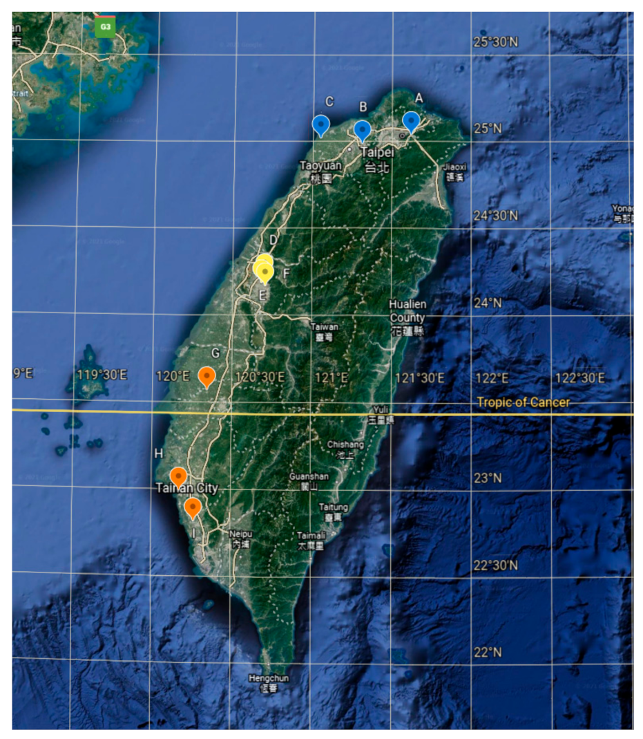
This study mainly focuses on the solar PV power plant in Taiwan. The declaration of the Renewable Development Act, the purpose of which was to encourage the usage of renewable energy, will promote energy diversification, improvement of energy building, mitigate the effect of greenhouse gases, develop the quality of the environment, support related business sectors, and improve sustainable development for the future [18]. The existing solar PV power plants are measured and set as a benchmark for improving the energy performance of the present and modern solar PV power plants. Different locations of the solar PV power plants in Taiwan are selected to evaluate the performance for 1 year from January to December 2020. The total of nine solar PV power plants studied includes three from the north, four from the middle, and another two from the southern part of Taiwan.

With renewable technologies increasing at a rapid rate to generate energy, the use of solar energy must be maximized in locations where solar radiation is accessible year-round. The use of energy for the production and installation of solar PV systems must be considered [19]. The numerous financial criteria, including the discount rate, effective discount rate, or rate of increase of energy costs, that influence the financial feasibility of the solar photovoltaic plant were examined. Furthermore, environmental factors for solar photovoltaic power generation, such as reducing carbon emissions and earning carbon credits, are also taken into account [20]. In addition, based on real data analysis, solar power plant performance may be assessed using IEC 61724 standards and an established model consisting of a photovoltaic array, battery storage system, controller, and converter [21,22]. If all of the essential data were accessible, it would be feasible to assess the performance of a single plant effectively. In industrial efficiency assessments, the DEA approach is often applied since it may provide a reasonable, objective, and reliable assessment [23].

To meet the growing energy demand of Taiwan, a highly effective approach is to exert extra support in renewable energy resources and technologies because of the huge amount of renewable energy sources, in particular solar energy, which is the focus of this research. At present, many studies use DEA to evaluate the performance of renewable energy. At the micro-level, scientists are focusing on improving the external influences on photovoltaic transformation efficiency and performance ratio, including weather, dust buildup, and other environmental variables that may impair PV system performance. Most articles focus on economic, policy, technology, resources, market, and industry issues for empirical research at the macro level. In addition, the common method used is a radial model or non-radial model of DEA. Each model has its shortcomings. The radial model simply analyzes the changes in input or output proportionately and does not take into account the development of slack. The slack measurement of the non-radial model does not account for variations in the input and output ratio. In this study, the authors used an epsilon-based measure efficiency model which connects radial and non-radial models. This model measures the performance efficiency of generated output energy from nine solar PV power plants in Taiwan using the limited amount of data available, such as the number of modules, ambient temperature, module temperature, plant capacity, irradiation, and generated energy. The results will be strategically important to assist government and private sectors, managers, designers, investors, and industries that need to make investment decisions. It also contributes to the evaluation of the performance efficiency of the selected solar PV power plant.

The study is organized as follows: Section 2 briefly explains the fundamentals of the DEA method and data collection. Section 3 discusses the methods and data envelopment analysis using the epsilon-based measure of efficiency. Section 4 presents the results and discussion. Lastly, Section 5 provides the conclusion of this study.

2. Materials

2.1. Data Envelopment Analysis

According to the principle of maximum input and output benefit, DEA utilizes the idea of relative efficient frontier theory to explain the performance of every single target DMU that is evaluated and assists in differentiating the most efficient and ideal weights [24]. DEA is a systematical model that was originally established by Charnes, Cooper, and Rhodes (CCR), according to the basic theory of the non-parametric approach for assessing technical efficiency [25], whose field of analysis is a set of DMUs that is capable of attaining multiple inputs and outputs. DEA is a recognized method that is established for several models and used in various fields by a significant number of researchers. Numerous developments have been established, starting with the first CCR model introduced, the same as the piecewise linear frontier which exhibits variable returns to scale (VRS) of the Banker, Charnes, and Cooper (BCC) model [26], which particularly enhances the limitation of the constant returns to scale (CRS) of the CCR model. The slacks-based measure (SBM) model is an additive DEA model that maximizes the total of the input and output that directly deals with the excess input and output deficit [27]. DEA usually has two parameters of technical efficiency, the radial and non-radial measurement [23]. To be able to deal with the difficulty associated with radial and non-radial models concerning the assumption of equivalent reduction around input and output indicators, the epsilon-based measure (EBM) model integrates both radial and non-radial models in a combined structure [28]. Moreover, there is certainly no requirement and no need to take into consideration, for creating a production function model, ahead and the unit conversion of factors, respectively [24,25,26,27,28]. For the input and output-oriented model, the inputs were minimized for a required quantity of output to be attained [29,30,31,32,33,34,35,36].

2.2. Data Collection

In this study, nine DMUs were selected in Taiwan.

Table 1. List of Solar PV power plants.

DMU	Site Number	Location	Type of Installation
A	1150041	Nangang District, Taipei City	ground-mounted
B	3300201	Taoyuan District, Taoyuan City	rooftop
C	3270101	Xinwu District, Taoyuan City	floating
D	4270011	Tanzi District, Taichung City	rooftop
E	4060061	Beitun District, Taichung City	rooftop
F	4110021	Taiping District, Taichung City	rooftop
G	6160011	Xingang Township, Chiayi County	rooftop
H	7080011	Anping District, Tainan City	rooftop
I	8200051	Gangshan District, Kaohsiung City	rooftop

shows the location, site number, and type of installation of every DMU. Seven evaluation indicators of solar PV power plant performance were used, and input and output indicators are shown in

Table 2. Input and output indicators.

DMU	(I1) Surface Area (m2)	(I2) Number of Module	(I3) Ambient Temperature (°C)	(I4) Plant Capacity (kWp)	(I5) PV Module Temperature (°C)	(I6) Irradiation (kWh/m2)	(O1) Generated Energy (kWh)
A	5181.24	3216	32.73	980.88	28.87	1079.452116	920,852
B	1235.55	768	30.27	234.24	27.22	1123.415085	289,700
C	2627.67	1632	32.64	481.44	28.83	1422.978564	644,478
D	1622.97	1008	34.35	307.44	26.05	1494.447055	416,246
E	1011.76	528	32.77	161.04	34.86	1511.717331	233,125
F	115.93	72	32.47	18.00	26.05	1468.902530	24,217
G	1546.6	960	32.53	283.20	32.57	1596.147420	425,225
H	3061.05	1900	31.82	494.00	31.99	1536.464182	759,626
I	7965.18	4896	34.06	1444.32	35.62	1631.734180	2,098,949

. The input indicators include surface area, number of modules, ambient temperature, plant capacity, and irradiation, while the output indicator includes the generated energy. Among them, the five indicators were obtained from Tatung Forever Energy Co., Ltd. Data were collected as follows. First, the solar irradiation and temperature were measured by a pyranometer and thermocouple, which are collected by a data logger. Then, these data were collected from inverters and other sensors through Modbus remote terminal unit (RTU) protocol by a smart gateway. Lastly, data was sent to a cloud system every 5 min and stored in a local gateway for edge computing. After that, surface area, number of modules, and plant capacity were collected based on the design of each solar PV power plant, while the ambient temperature was collected from the adjacent weather station on each solar PV plant. The solar PV power plants were developed between 2017 and 2018, and they all employ the same technology. Furthermore, in this study, nine solar PV power plants employed four busbars of polycrystalline solar cells in modules. The descriptions of the input and output indicators used in the evaluation shown in Table 2 are as follows:

I1 Surface area is defined as the gross size of the modules and measured in square meters (m²).

I2 Number of module is the quantity of solar PV modules installed.

I3 Ambient temperature is the annual average temperature of the solar PV power plant’s surroundings, measured in degrees Celsius (°C).

I4 Plant capacity is the aggregate unit capacity of all solar PV modules in the plant and measured in kilowatt-hour (kWh).

I5 PV module temperature is the annual average temperature of a solar PV module, measured in degrees Celsius (°C).

I6 Irradiation is the total radiation received on a surface with a defined tilt angle and measured in kilowatt-hour per meter squared (kWh/m²)

O1 Generated energy is the annual solar energy output of a photovoltaic system and measured in kilowatt-hour (kWh).

Table 1 presents the list of solar PV power plant locations as demonstrated in Figure 1. DMUs A, B, and C were from the northern part of Taiwan, where A was ground-mounted, B was installed on the rooftop, and C was installed floating. Then, DMUs D, E, F, and G were from the middle part of Taiwan and were installed on rooftops. Lastly, DMUs H and I were from the southern part of Taiwan and installed on rooftops. Each solar PV power plant will be evaluated for its performance in this study.

3. Research Methodology

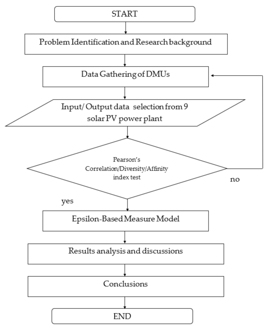
The current study used the epsilon-based measure model to evaluate the performance efficiency of nine solar PV power plants in Taiwan. The EBM model research flow chart of this present study is depicted in Figure 2. The study began with problem identification and research background. Next, data gathering of DMUs was conducted from nine different solar PV power plants in Taiwan. First, inputs and output were selected to evaluate the performance of the solar PV power plants. Next, Pearson’s coefficient was used to test the correlation of the input and output indicators. Based on the typical Pearson’s correlation coefficient, it presents the translation of the source in assessing correlations. However, the EBM model in this study uses a different correlation matrix that evaluates the affinity of two vectors without translating the source. The diversity and affinity index is evaluated before applying the EBM model. Then, the epsilon-based measure input-oriented under constant return to scale (EBM I-C) model was applied to evaluate the performance of the nine solar PV power plants from January to December of the year 2020. After that, the results analysis and discussion of the performance of DMUs every month were conducted. Finally, the empirical result and conclusion were discussed.

3.1. Epsilon-Based Measure Model

The DEA model is divided into two parts: (1) radial models, described by the CCR and BCC models, and (2) non-radial models described by the SBM model. Each model has its shortcomings. The radial model only considers the proportionate change in input or output and disregards the appearance of slacks, while the measurement of the non-radial model faces slacks and does not deal with the proportion of input and output changes. These two types of efficiency measurement have unique advantages which are unacceptable to evaluate other situations. The epsilon-based measure (EBM) model has been developed to overcome the shortcomings regarding the proportionality of the input and output indicators changes. In this study, the EBM model is used which has the characteristics of both radial and non-radial models in a combined structure. The scalar and vector parameters are included in this structure and must satisfy the condition of affinity matrix when the largest eigenvalue and eigenvector are from 0 to 1. These two parameters are incorporated in the EBM model to evaluate the performance of the DMUs with regard to the efficiency score.

By way of implying the input-oriented EBM (EBM-I-C) for ${\mathrm{DMU}}_0=\left(x_0,y_0\right)$, it is calculated as

$$\underset{\theta ,\lambda ,s^{-}}{{\gamma }^{*}=\min } \theta -{\epsilon }_x{\displaystyle \sum }_{i=1}^m\frac{w_i^{-}{s}_i^{-}}{x_{i0}},$$

(1)

subjected to

$$\theta x_0-X\lambda -s^{-}=0,\hspace{1em}\hspace{1em}Y\lambda \ge y_0,$$

(2)

$$\lambda \ge 0,\hspace{1em}\hspace{1em}{s}^{-}\ge 0,$$

(3)

where the formulation ${\gamma }^{*}$ is obtained as the optimum within separating value between the radial $\theta$ and non-radial slacks term ${{\displaystyle \sum }}_{i=1}^m\frac{w_i^{-}{s}_i^{-}}{x_{i0}}$, $w_i^{-}$ is the weight input $\left(i\right)$ and satisfies ${{\displaystyle \sum }}_{i=1}^m{w}_i^{-}=1\left(w_i^{-}\ge 0 \forall \right)$, and $s_i^{-}$ is the quantity of slack in the input $\left(i\right)$. The radial $\theta$ and non-radial slacks terms are combined by ${\epsilon }_x$ which is a key parameter that varies on the scattering of the inputs.

3.2. Diversity and Affinity Indexes

In accordance with the fundamental principle of Pearson’s correlation coefficient, the condition is $-1\le P\left(a,b\right)\le +1$, where $P\left(a,b\right)$ is the Pearson’s correlation coefficient. In this regard, the lowest correlation between input and output indicators is the Pearson’s coefficient closest or equal to -1 while the Pearson’s coefficient that is closest or equal to 1 is the highest correlation among the input and output indicators. However, it is not guaranteed that the principal vector will result in positive components. Although it is possible to adjust the Pearson’s coefficient into a limit of $0\le P\left(a,b\right)\le +1$, this can lead to a positive skew distribution, since the condition is greater than or equal to zero but less than or equal to one of the Pearson’s correlations that makes it positive in the DEA model.

Regarding the ${\epsilon }_x$ and $w_i^{-}$ in the EBM model in DEA, the values of these two are the most important for determining the impact of input indicators on the output indicators [38]. Since the EBM model varies depending on the degree of data dispersion, when ${\epsilon }_x$ is equal to 0 this indicates low dispersion on the data, while ${\epsilon }_x$ that is equal to 1 means high dispersion on the data. It must also take into consideration that value of $w_i^{-}$ varies on the affinity between the inputs, this only means that a higher degree of affinity between the inputs, the higher weights are allotted to the inputs. Still, the EBM model used an affinity index between two vectors as an alternative to Pearson’s correlation coefficient.

The two positve vectors ($ϵR_{+}^n$ and $bϵR_{+}^n$) by a component $n$ represent the observed values for a specific input element in DMUs. The affinity index $S\left(a,b\right)$ between vectos $a$ and $b$ with the following characteristics:

• $S\left(a,a\right)=1\left(\forall \_a\right)$—identical,
• $S\left(a,b\right)=S\left(a,b\right)$—symmetric,
• $S\left(ta,b\right)=S\left(a,b\right)\left(\forall t>0\right)$—units-invariant, and
• $1\ge S\left(a,b\right)\ge 0\left(\forall a,b\right)$.

Let us define

$$c_j=\ln \frac{b_j}{a_j}\left(j=1,\dots ,n\right),$$

(4)

$$\overline{c}=\frac{1}{n}{{\displaystyle \sum }}_{j=1}^n{c}_j,$$

(5)

$$c_{max}=\underset{j}{\max }\left\{c_j\right\},$$

(6)

and

$$c_{min}=\underset{j}{\min }\left\{c_j\right\},$$

(7)

where $\left(a,b\right)$ is diversity index of vectors, $\left\{c_j\right\}$ is the deviation, and $\overline{c}$ is the average that is identified in this way:

$$D\left(a,b\right)=\frac{{{\displaystyle \sum }}_{j=1}^n\left|c_j-\overline{c}\right|}{n\left(c_{max}-c_{min}\right)}=0,$$

(8)

if

$$(c_{max}=c_{min}),$$

(9)

and

$$0\le D\left(a,b\right)=D\left(b,a\right)\le \frac{1}{2},$$

(10)

$D\left(a,b\right)$ is equals to 0 only if vectors $a$ and $b$ are proportional. However, when it denotes an affinity index $S\left(a,b\right)$ that is between vectors $a$ and $b$, then

$$S\left(a,b\right)=1-2D\left(a,b\right)$$

(11)

but when the condition is $1\ge S\left(a,b\right)\ge 0,$ the affinity index $S\left(a,b\right)$ is accomplished along with Equations (1) and (5).

The Pearson’s correlation coefficient ($P\left(a,b\right))$ in the DEA model is computed with the equation:

$$P\left(a,b\right)=\frac{{{\displaystyle \sum }}_{j=1}^n\left(a_j-\overline{a}\right)\left(b_j-\overline{b}\right)}{{{\displaystyle \sum }}_{j=1}^n{\left(a_j-\overline{a}\right)}^2-{\left(b_j-\overline{b}\right)}^2},$$

(12)

where $\overline{a}$ and $\overline{b}$ are the respective averages of $a_j$ and $b_j$.

However, the normal way of computing the Pearson’s correlation coefficient $P\left(a,b\right)$ in the DEA model is replaced by the affinity index in the EBM model. Then, the Pearson’s correlation coefficient $P\left(a,b\right)$ is greater than or equal to negative one but less than or equal to 1 will be adjusted to the condition that $P\left(a,b\right)$ is greater than or equal to zero but less than or equal to one.

4. Results and Discussions

Results of the evaluation from the nine solar PV power plants using the epsilon-based measure model are analyzed and discussed in this section.

Evaluating the Performance of DMUs

The EBM model was employed for the input and output indicators for the year 2020 to evaluate the performance efficiency, as well as ranking, by means of the generated annual energy of solar PV power plants in Taiwan.

For DEA to work, the selected input and output variables must have an isotonic relationship. The isotonic condition does not require an inconsistent relationship between the inputs and outputs. Therefore, the output level is at least the same and does not decrease when inputs increase in order to ensure that the input and output variables comply with this isotonic requirement. The Pearson’s correlation analysis is used to confirm a positive correlation between the selected inputs and outputs of each DMU. If the coefficient variables are negative, the input and output variables must be changed. The result presented in

Table 3. Correlation of Input and Output.

	Surface Area (m2)	Number of Module	Ambient Temperature (°C)	Plant Capacity (kWp)	PV Module Temperature (°C)	Irradiation (kWh/m2)	Generated Energy (kWh)
Surface Area (m2)	1	0.999734	0.402811	0.998134	0.486877	0.046868	0.975711
Number of module	0.999734	1	0.398011	0.998271	0.471723	0.039358	0.974330
Ambient Temperature (°C)	0.402811	0.398011	1	0.409356	0.204303	0.528529	0.434766
Plant Capacity (kWp)	0.998134	0.998271	0.409356	1	0.454921	0.011250	0.967319
PV Module Temperature (°C)	0.486877	0.471723	0.204303	0.454921	1	0.525448	0.552190
Irradiation (kWh/m2)	0.046868	0.039358	0.528529	0.011250	0.525448	1	0.217323
Output Energy (kWh)	0.975711	0.974330	0.434766	0.967319	0.552190	0.217323	1

shows that input and output indicators were in positive values. It indicates that all the data indicators were acceptable to run using the EBM model. In addition, the lowest and highest correlation coefficient among the input and output indicators were irradiation with a value of 0.217323 and surface area with a value of 0.975711, respectively. This shows that input variable surface area (I1) has a strong correlation with the output variable generated energy (O) compared to the irradiation that shows a low correlation with the output variable (O).

In order to ensure that the input and output variables were corresponding to the efficiency evaluation of EBM in the DMUs, the affinity and diversity indicators were used. The result is shown in

Table 4. Affinity Matrix.

	Surface Area (m2)	Number of Module	Ambient Temperature (°C)	Plant Capacity (kWp)	PV Module Temperature (°C)	Irradiation (kWh/m2)
Surface Area (m2)	1	0.61167	0.61090	0.28559	0.59123	0.59241
Number of module	0.61167	1	0.60274	0.41987	0.58004	0.58409
Ambient Temperature (°C)	0.61090	0.60274	1	0.61945	0.44662	0.44839
Plant Capacity (kWp)	0.28559	0.41987	0.61945	1	0.59337	0.60418
PV Module Temperature (°C)	0.59123	0.58004	0.44662	0.59337	1	0.48455
Irradiation (kWh/m2)	0.59241	0.58409	0.44839	0.60418	0.48455	1

and

Table 5. Diversity Matrix.

	Surface Area (m2)	Number of Module	Ambient Temperature (°C)	Plant Capacity (kWp)	PV Module Temperature (°C)	Irradiation (kWh/m2)
Surface Area (m2)	0	0.19416	0.19455	0.35720	0.20439	0.20379
Number of module	0.19416	0	0.19863	0.29006	0.20998	0.20795
Ambient Temperature (°C)	0.19455	0.19863	0	0.19028	0.27669	0.27581
Plant Capacity (kWp)	0.35720	0.29006	0.19028	0	0.20332	0.19791
PV Module Temperature (°C)	0.20439	0.20998	0.27669	0.20332	0	0.25772
Irradiation (kWh/m2)	0.20379	0.20795	0.27581	0.19791	0.25772	0

, where the input and output indicators comply with the requirement of the EBM model for affinity index and diversity index that have a condition of $0\le P\left(a,b\right)\le 1$ and $0\le D\left(a,b\right)=D\left(b,a\right)\le 1/2$, respectively. When both vectors were proportional, it was only equal to 0. This shows that the EBM model was fit for evaluating the performance scores of the selected 9 DMUs, according to the established conditions.

The weight $(w_i^{-})$ of the inputs and outputs indicators and the epsilon $({\epsilon }_x)$ was a key part in removing the EBM score for every DMU. The weighted index identifies the proportionate effect of input indicators on the output indicators. The entire weighted indexes are positive, as shown in

Table 6. Weight to Input or Output.

Surface Area (m2)	Number of Module	Ambient Temperature (°C)	Plant Capacity (kWp)	PV Module Temperature (°C)	Irradiation (kWh/m2)
0.167447	0.172449	0.168310	0.157611	0.166636	0.167547

. Corresponding to the results, it indicates that a small adjustment within the input indicators will affect output indicators to change, and this means that the input indicator is directly proportional to the output indicator, when the input indicator increased the output indicator also increased.

The epsilon for EBM is equal to 0.461214, which satisfies the condition $0\le epsilon index\le 1$. The efficiencies of the nine solar PV power plants were derived from the weight and epsilon of the EBM model.

For a DMU to obtained the first ranking, it means that theta ($\theta$) needed to be equal or near to 1, and all slacks in every variable were the lowest or near to 0. On the contrary, if the slack was high and the $\theta$ was far from 1, the DMU could not reach the highest ranking. In the case when $\theta$ was higher than 1, this means that the DMU was inefficient. In this regard, the values of inputs needed to be adjusted appropriately to enhance the performance efficiency and the output indicators. It can be observed in

Table 7. Theta and slacks of DMUs and input and output indicators.

		Slack 1	Slack 2	Slack 3	Slack 4	Slack 5	Slack 6	Slack 7
DMU	Theta (θ)	(I1) Surface Area (m2)	(I2) Number of Module	(I3) Ambient Temperature (°C)	(I4) Plant Capacity (kWp)	(I5) PV Module Temperature (°C)	(I6) Irradiation (kWh/m2)	(O1) Generated Energy (kWh)
A	0.674450	0	21.055903	7.134911	27.901807	3.844150	12.161335	0
B	0.889778	0	7.596787	22.229847	9.074551	19.303445	774.376193	0
C	0.930746	0	15.669994	19.923545	4.622648	15.893462	823.410364	0
D	0.973270	0	10.122306	26.677657	12.796641	18.289820	1130.908459	0
E	1.029899	157.337602	0	29.963569	5.437864	31.946040	1375.682875	0
F	0.874933	3.844252	2.422892	27.391849	0	21.772167	1236.209065	0
G	1.043361	0	9.748188	27.035448	2.875715	26.766022	1334.785369	0
H	1.058119	356.293692	238.525075	21.339835	0	20.958063	1035.224246	0
I	1	0	0	0	0	0	0	0

that five out of the nine DMUs were less than 1, including DMU A, B, C, D, and F, while DMU E, G, and H were greater than 1, which indicates these DMUs are inefficient. Table 7 also describes the $\theta$ and slacks in the solution for each DMU. In this regard, DMU I having $\theta$ equal 1 and every slack equal to 0 makes it efficient compared to other DMUs.

Among the nine DMUs, only DMU I performed efficiently and scores 1, which makes it rank 1, while the rest of the DMUs scored from 0.643837 up to 0.884663, which makes these DMUs less efficient compared to DMU 1 as shown in

Table 8. Score and ranking of DMUs.

No.	DMU	Score	Rank
9	I	1	1
8	H	0.884663	2
7	G	0.849509	3
5	E	0.803696	4
4	D	0.796720	5
3	C	0.794814	6
2	B	0.721392	7
6	F	0.674935	8
1	A	0.643837	9

.

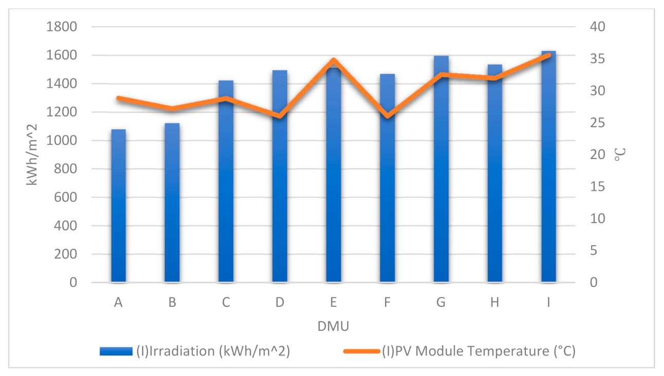
According to Figure 3, the top three DMUs having the highest irradiation received on the specific solar PV power plant station were I, G, and H, having an irradiation range from 1536.46 to 1631.73 kWh·m⁻², which are all located in the middle and southern part of Taiwan. Then, the next three DMUs were E, D, and F, having an irradiation value range of 1468.90 to 1511.72 kWh·m⁻², all of which are from the middle part of Taiwan. Finally, the three remaining DMUs were the lowest among the other six DMUs, being A, B, and C and having an irradiation value of 1079.45 to 1422.42 kWh·m⁻², all of which are from the northern part of Taiwan. In addition, those that had temperatures of their PV modules higher than 30 °C were DMUs I, E, G, and H, which are from the middle and southern part of Taiwan, while DMUs A, B, C, D, and F had a PV module temperature lower than 30 °C, and are from the middle and northern part of Taiwan.

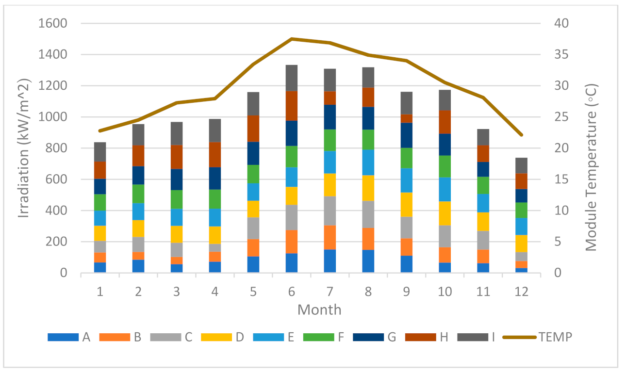
The generated energy from January to December of the nine DMUs is shown in Figure 4; the accumulated energy of the nine DMUs that was lower than 400,000 kWh were produced during November and December, the totals higher than 400,000 kWh but not more than 500,000 kWh were produced during January, February, March, April, and October, and then the months that produced more than 500,000 kWh of energy were May, June, July, August, and September. The seasons in Taiwan are divided into four. Winter runs from December to February, spring is from March to May, summer is from June to August, and autumn is from September to November [39], which is demonstrated from the data in Figure 5. This also shows that the summer season had the highest total irradiation and average module temperature, while the autumn season had the lowest. The data distribution for the entire year of 2020 alone indicates that irradiance and module temperature has a major effect on solar PV power plant power output. Seasonal changes had a great effect on irradiation and temperature that significantly affected the PV power generated and efficiency [40].

5. Conclusions

The rapid economic growth in Taiwan led to a significant rise in energy consumption which in turn led to the Renewable Development Act. The target of 27 GW of renewable energy capacity in the year 2025 is a significant challenge to Taiwan. The use of sustainable energy that will meet the present needs without compromising the needs until 2025 will help the energy requirements of Taiwan. The 20 GW of solar energy capacity that will be built, out of 27 GW of renewable energy capacity, will be a significant challenge. Therefore, Taiwan needs to improve and sustain existing solar PV energy to increase and maintain the production of energy demand. This study proposed an epsilon-based measure (EBM) model in DEA to evaluate the performance of the existing nine solar PV power plants in Taiwan. Then, the EBM model was assigned and used to evaluate the DMUs’ performance in energy production by way of providing the efficiency scores and rankings for the power plant company improvement. The empirical results will help assist the plant managers in identifying their perspective with the existing plant performance and making viable future advancement solutions. The results also indicate the usefulness of the EBM model in DEA, in which the model will be able to evaluate the performance of DMUs and contribute to the solutions of the company. Additionally, the result shows that solar PV power plants located near the equator perform better. This study can be used as a basis in different fields for evaluating performance. Even though the study has achieved the set goals, various restrictions are present. The limitation of this study focuses on the micro and macro-level factors that affect the performance of the solar PV power plants, which is based on the long-term monitoring goals and vision. Examples of micro-level factors are weather, dust buildup, and other environmental variables, while macro-level factors are economic, policy, technology, resources, market, and industry issues. For future evaluation of performance, these shortcomings can be addressed by the addition of DMU and the links at the micro and macro-level that influence the performance of the solar PV plants. Furthermore, intelligent technologies are evolving and capable of gathering real-time data sent between stakeholders and operations managers [41]. A future study might expand the number of years of solar PV plant data that can be analyzed and examined, and even the performance of the past and present states, and could make the activities smart for optimizing decision making by creating artificial intelligence.