Resilience Assessment of Wind Farms in the Arctic with the Application of Bayesian Networks

Abstract

Infrastructure systems, such as wind farms, are prone to various human-induced and natural disruptions such as extreme weather conditions. There is growing concern among decision makers about the ability of wind farms to withstand and regain their performance when facing disruptions, in terms of resilience-enhanced strategies. This paper proposes a probabilistic model to calculate the resilience of wind farms facing disruptive weather conditions. In this study, the resilience of wind farms is considered to be a function of their reliability, maintainability, supportability, and organizational resilience. The relationships between these resilience variables can be structured using Bayesian network models. The use of Bayesian networks allows for analyzing different resilience scenarios. Moreover, Bayesian networks can be used to quantify resilience, which is demonstrated in this paper with a case study of a wind farm in Arctic Norway. The results of the case study show that the wind farm is highly resilient under normal operating conditions, and slightly degraded under Arctic operating conditions. Moreover, the case study introduced the calculation of wind farm resilience under Arctic black swan conditions. A black swan scenario is an unknowable unknown scenario that can affect a system with low probability and very high extreme consequences. The results of the analysis show that the resilience of the wind farm is significantly degraded when operating under Arctic black swan conditions. In addition, a backward propagation of the Bayesian network illustrates the percentage of improvement required in each resilience factor in order to attain a certain level of resilience of the wind farm under Arctic black swan conditions.

1. Introduction

Infrastructure systems in the Arctic are prone to disruptions in their operation caused mainly by the harsh weather conditions they face. The resilience of infrastructure systems in the face of disruptions and the resulting consequences has become a significantly recognized topic among project owners. The author in [1] defined system resilience as the extent to which a system maintains a minimum level of performance in the face of disruptions. Wind farms (WFs) are among the infrastructure systems installed in the Arctic that are prone to disruptions resulting from the weather conditions in the region. Ice accretion on the blades of wind turbines (WTs), snow accumulation that blocks the roads to WFs and prevents maintenance procedures, and cold temperatures that limit the dexterity of the WF staff are among the disruptions that affect the resilience of WFs in the Arctic.

When uncertainties are taken into consideration in resilience analyses, probabilistic resilience measures that normally have a probability value between 0 and 1 can be used [2]. For example, a system that possesses a resilience estimate of 0.8 can indicate that the system is, in general, 80% resilient against a specific disruptive event. Furthermore, it could reflect an 80% probability that the system will continue to perform under a defined disruptive event, or recover to an acceptable system performance level, within a given time interval after the disruptive event disappears.

Due to the uncertainty in energy system applications such as WFs, there are several variables that have to be determined and many explicit pieces of evidence that can be linked together through the application of Bayesian networks (BNs), which depend on the concept of probability to compute uncertainties. BNs have been used for modeling infrastructure resilience [3,4,5], post-disaster infrastructure recovery [6], and in applications of infrastructure system reliability [7,8].

According to Aven [9], resilience is event-dependent, and can be assessed based on the description of the disruptive event that the infrastructure system is facing. In that sense, there is a need to define the type of events that the system deals with, in order to decide whether it is resilient to them or not. Therefore, the approach adopted in this paper is to define three separate scenarios against which the resilience of a WF can be tested. The first scenario is the baseline scenario, where the WF is operating under normal operating conditions, while the second scenario tests the WF’s resilience to Arctic operating conditions on the WF site. The third scenario is an imaginable scenario, defined as an Arctic black swan scenario, where the impacts of the disruptions are extreme.

The black swan concept was defined and popularized by Nassim Nicholas Taleb in his book The Black Swan [10], in which he identified three main attributes of a black swan event: (1) a black swan event is an outlier and unexpected, in the sense that nothing in the past can indicate the likelihood of it occurring; (2) its impact is extreme; and (3) after a black swan event has occurred, humans are able to find an explanation for it, making it explainable and predictable despite its outlier nature. According to Aven [11], black swan events are seen as extreme events relative to current knowledge and beliefs. Furthermore, Aven and Krohn [12] pointed out that black swan events can be events that are known to the risk analysts, but assessed to have a negligible probability of occurrence, and thus not anticipated to happen. Therefore, testing a WF’s resilience to black swan events helps the WF operator to be prepared for worst-case scenarios.

This study is motivated by the observation that uncertainties emerging from the changing climate conditions might open up the possibility for unexpectedly harsh weather conditions, characterized as a black swan, to take place in regions such as the Arctic. The effects of such a scenario taking place, and affecting the operation of WFs in the Arctic, are not well addressed in the literature. Using BNs to model an uncertainty scenario and calculating the resulting resilience is effective as a BN is a practical tool for calculating conditional probabilities, and it is easy to understand its models. Most studies that have implemented BNs for applications in the Arctic are concerned with risks posed to ship transportation and collisions with ice in Arctic waters [13,14,15]. WF systems are relatively new in the Arctic, and as there is a corresponding lack of data in the field, the use of BNs to describe Arctic scenarios and their effects on WFs can be an interesting application.

This paper utilizes BNs to estimate the resilience of WFs located in the Arctic region of Norway, which will contribute towards enriching the literature with a unique methodology, to create multiple scenarios and assess the WF resilience against each scenario. The paper includes and assesses the WF’s resilience against three main scenarios, which are the normal operating conditions scenario, the Arctic operating condition scenario, and the Arctic black swan scenario.

The remaining sections of this paper are organized as follows: Section 2 presents a conceptual definition of engineering resilience. Section 3 introduces the methodology adopted, while Section 4 explains the design and modeling of the BN. Section 5 demonstrates the use of the proposed BN by applying it to a case study of a WF in the Norway Arctic region. The conclusions of the study are then presented in Section 6.

2. Conceptual Definition of Engineering Resilience

Youn et al. [16] proposed a theoretical definition of engineering resilience, which derives its generic formula from the system reliability and the three key attributes of prognostics and health management (PHM) efficiency, which are diagnostics, prognostics, and condition-based maintenance [17]. The definition concluded that resilience can be mathematically measured as the sum of reliability and restoration, as per Equation (1) [16].

Resilience (Ψ) = Reliability (R) + Restoration (ρ)

(1)

Restoration (ρ) is defined as “the event at which the ‘up’ state is re-established after failure” [18], which according to [16] depends mainly on the attributes of PHM efficiency and system reliability, by focusing on transforming the system into a resilient system and minimizing its life-cycle cost (LLC). Based on that, restoration can be expressed as the joint probability of a system failure event (i.e., the reliability of the system) (Esf), and the three PHM attributes, which are a correct diagnosis event (Ecd), a correct prognosis event (Ecp), and a mitigation/recovery (M/R) action success event (Emr), expressed in Equation (2) [16].

Restoration (ρ) = P (E_sf E_cd E_cp E_mr)

(2)

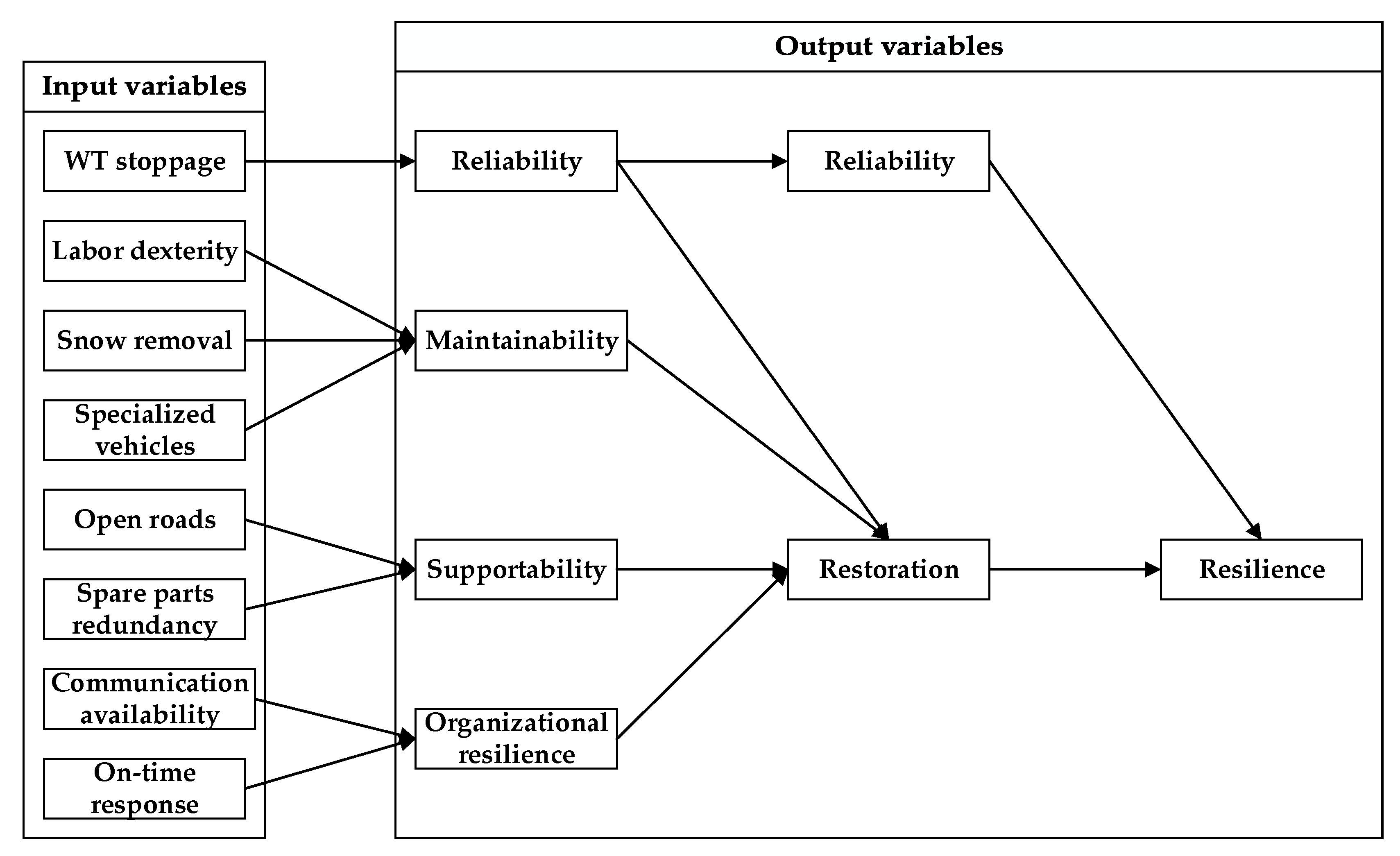
The authors in [19] proposed that the most important factors for consideration in assessing the resilience of a system in the Arctic are: (I) reliability of the system’s components, (II) maintainability of disrupted components, (III) supportability of maintenance activities, (IV) the organizational resilience, and (V) the PHM efficiency of the system. However, the PHM elements, namely diagnosis, prognosis, and M/R action, are embedded in the maintainability, supportability, and organizational factors of restoration. This is because the organization has to gather and analyze data in order to define the potential hazards (diagnosis), estimate the remaining useful life of the impacted WT components (prognosis), and take the required M/R measures in a condition-based maintenance (CBM) sense, where the latter can be reflected by the maintainability and supportability of the WF. Based on that, and by referring to restoration equation in [19], restoration can be expressed as in Equation (3).

Restoration (ρ) = (1 − R) × M × S × O

(3)

where R, M, S, and O are the conditional probabilities of reliability, maintainability, supportability, and organizational resilience, respectively, which are the main factors of resilience that are important for WFs to maintain and regain their resilience during and after a disruptive event. These factors can be denoted as output variables that will depend on other input variables in determining their values. Figure 1 illustrates the input and output variables that will shape the resilience of WFs, considering Equations (1) and (3), and that will be used in establishing the Bayesian network (BN) for calculating the resilience of the WFs.

2.1. Reliability

WF reliability reflects the ability of the WTs to operate as required, without failure, for a given period under given conditions. Reliability can be expressed in terms of the probability of failure [20], as in Equation (4):

R(t) = 1 − F(t)

(4)

where F(t) is the probability at which the WTs stop operating due to the hazards, which can be due to Arctic operating conditions or component degradation. Different statistical models have been developed for reliability modeling of complex systems like WTs, such as the Power law process (PLP), which is a special case of the Poisson process [21], and the Poisson process with covariates [22]. For the sake of simplicity, in this paper the Poisson distribution is used to represent the probability of the WT stoppage events, as shown in Equation (5) [23]:

$$\mathrm{p}(\mathrm{k};(0,\mathrm{t}),\mathsf{\lambda })=\frac{{(\lambda t)}^k}{k!}{e}^{-\lambda t}$$

(5)

where k is the number of WT stoppage events the Poisson distribution tries to find the probability of, over a fixed time interval (0, t). λ is the mean value of the distribution and is equal to the number of WT stoppage events over a specific period (e.g., a month).

2.2. Maintainability

The maintainability of an item is the ability to keep performing, or restored to a state to perform as demanded, under given conditions of operation and maintenance [18]. Maintainability is influenced by the design of the system, in terms of how easy it is to maintain it. From a different angle, the maintainability of a WF can be expressed in terms of two factors, which reflect the ability to restore the functionality of the WF: the level of labor dexterity when carrying out the maintenance activities, and the accessibility to the WF; both factors are affected by the Arctic operating conditions. In order to maintain access to the WTs, WFs can utilize snow-removing strategies, which might be costly, or equip the service team with specialized vehicles. A cost/benefit analysis must be carried out in order to determine which option is better. However, most WFs employ a combination of both solutions [24].

2.3. Supportability

Supportability is defined as the ability of a system to be supported to maintain a certain level of availability under defined operational conditions and given logistic and maintenance resources [18]. Based on this definition, the supportability of a WF involves the provision and availability of spare parts and tools that will help the service team to restore the WF’s performance and availability, during and after a disruptive event. To this end, supportability depends on the redundancy of spare parts, and the accessibility of roads and routes, via which spare parts and tools can be delivered by suppliers.

2.4. Organizational Resilience

According to the BS-65000 standard [25], organizational resilience implies the capacity of the organization to prepare for disruptive events, respond and adapt to them, whether they take the organization by surprise or unfold gradually. Cutter et al. [26] argue that organizational resilience requires an assessment of the physical properties of the organization, such as communication technology, number of members, and emergency assets. Hence, the resilience of a WF can be measured in terms of (I) communication availability and (II) on-time response to events.

• Communication availability (CA) covers the communication between staff members and the WF. Incidents involving loss of connection with WTs, which lead to loss of data, are stored in the SCADA system. A Poisson distribution can be used to estimate the probability of loss of connection events (x), taking place over a specific interval (0, t), considering an average number of loss of connection incidents (λ). Hence, the probability of connection availability can be represented as per Equation (6) [23]:

  $$\mathrm{CA}=1-\mathrm{p}(\mathrm{x};(0,\mathrm{t}),\mathsf{\lambda })=1-\frac{{(\lambda t)}^x}{x!}{e}^{-\lambda t}$$

  (6)
• On-time response to events covers the responsiveness of the operator to disruptive events and is a measure of the WF’s resilience, which can be assessed by the probability of an on-time response to the events that have led to WT stoppage. For example, if 85% or more of the disruptive events that lead to or require stopping the WTs are being handled and treated by the WF operator, within the first hour of their occurrence, the WF operator can be described as resilient, and the on-time response variable can be set at 100%, and considered successful [3]. This can also include corrective maintenance activities if the treatment of the failure starts within the first hour of its occurrence.

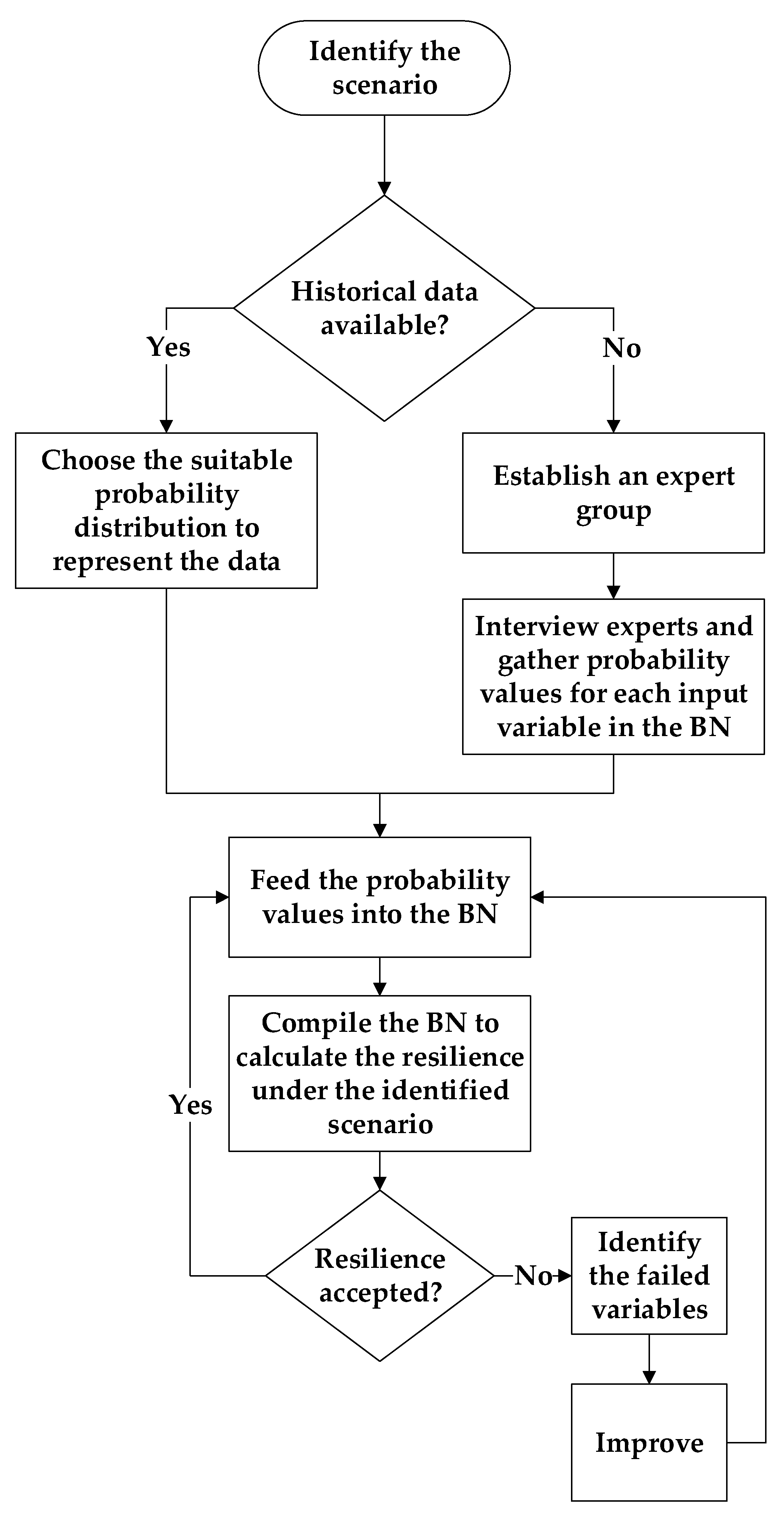
3. Methodology

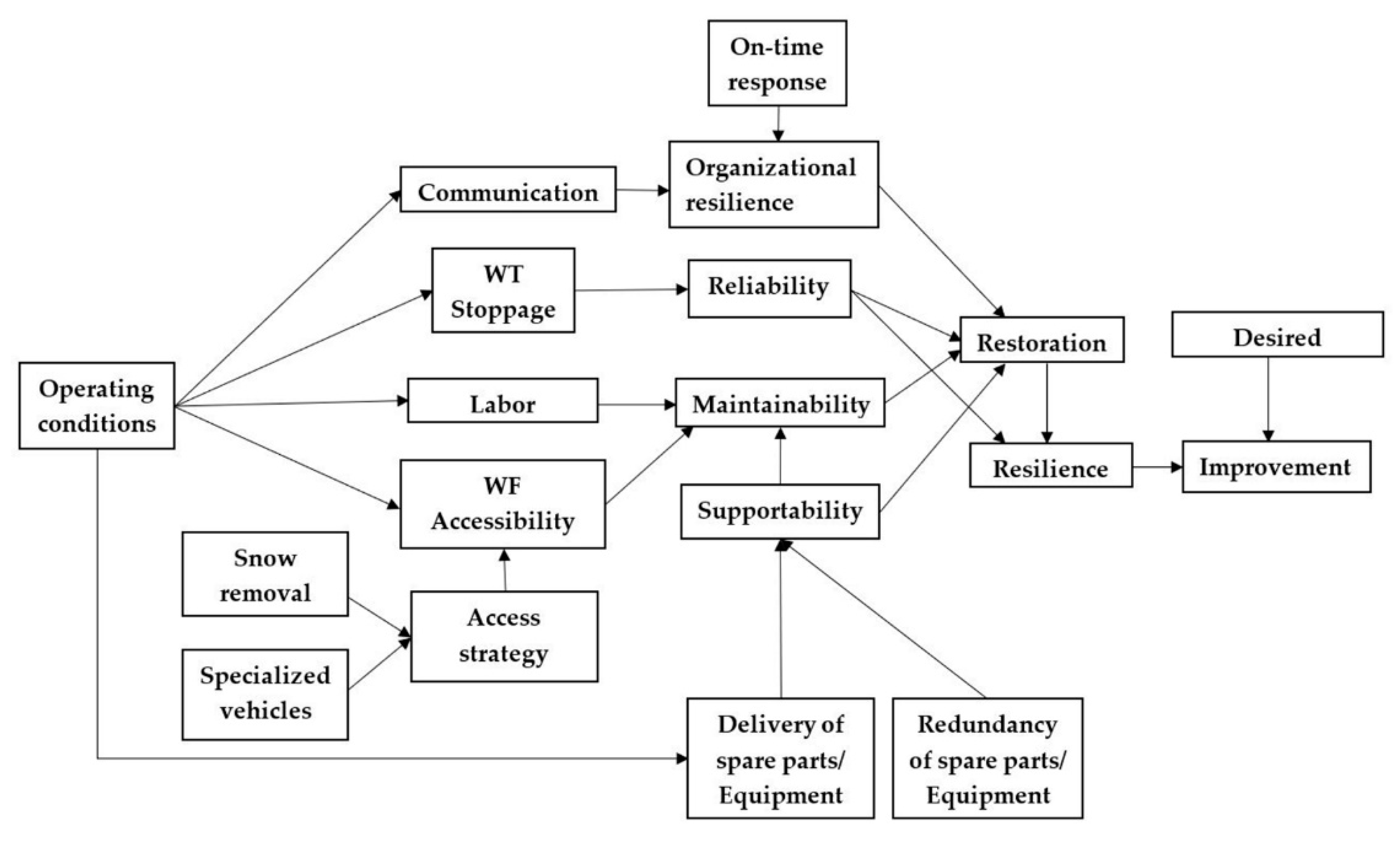
The methodology adopted to calculate resilience using the proposed BN is illustrated in Figure 2. The probability values of the input variables in the BN will either be extracted from historical data gathered from WFs or, in the event of a lack of data, from expert assessments. Afterwards, the BN is compiled to provide the posterior probabilities of the output variables, including resilience. Upon calculating the resilience value of the WF, the BN will show the probability of urgency to take measures to improve the WF resilience.

4. Designing the Bayesian Network

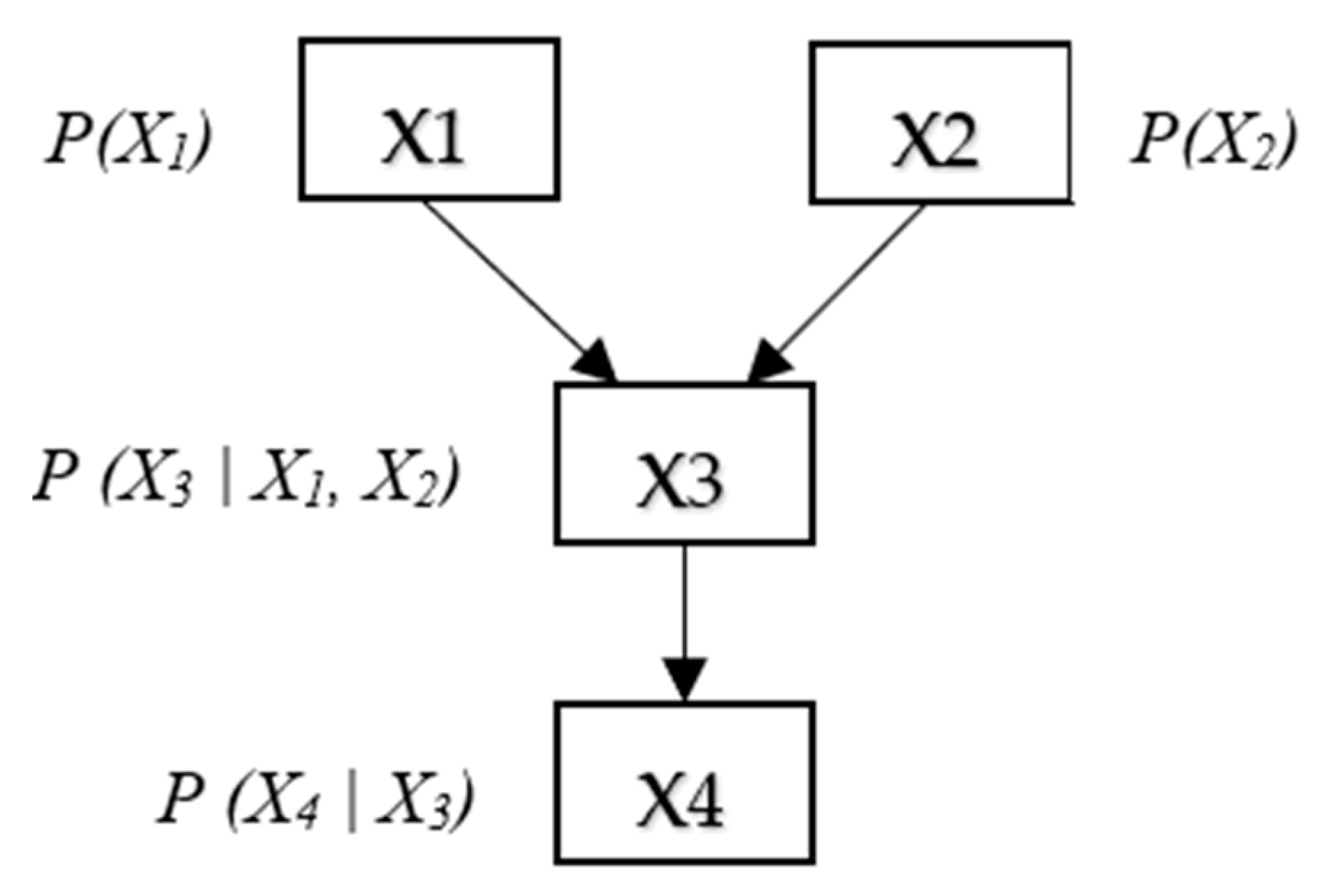
Graphically, a BN consists of nodes, and links that connect the nodes together. The nodes represent the variables, which can be an event or the state of a specific component, such as the state of failure or no failure of that component. Each node contains the probability of the occurrence of an event or state. The nodes are classified into parent nodes and child nodes, depending on how they are connected to each other in the graph, and which node is the predecessor (parent), and which the successor (child). The links in the BNs denote the causal relationship between the nodes. For example, in Figure 3, the nodes X1 and X2 are the parents of node X3, which is the child of both nodes. Likewise, node X3 is the only parent of node X4, which is its child.

BNs are described as directed graphs, which means that the relationships between the nodes are directed in one direction, with no cycles or links going backwards to the original (parent) node. A BN is an efficient tool for calculating the posterior probability of uncertain variables (the probability of the child nodes), depending on the known condition or the evident probability of other variables (the parent nodes), in what is known as the conditional probability, which updates the probabilities of events when given a certain condition or evidence.

The conditional relationships between the variables in a BN are measured by conditional probability distributions. Equation (7) presents the full joint probability distribution of a BN consisting of n variables X₁; X₂; …; X_n [3].

$$\mathrm{P}({\mathrm{X}}_1,{\mathrm{X}}_2,\dots ,{\mathrm{X}}_{\mathrm{n}})={{\displaystyle \prod }}_{i=1}^{n}P(X_i|Parents\left(X_i\right))$$

(7)

The variables/nodes used in modeling the BN are Boolean discrete variables, having values of (Yes/No), where the Yes state represents the success state of a specific variable, and the No state represents the fail state of that variable. For example, labor dexterity, which contributes to the successful maintenance of WTs, is reduced by 70% during the presence of extreme Arctic operating conditions. Therefore, assuming that labor dexterity has a 100% probability of being successful under normal operating conditions, the probability of successful labor dexterity is reduced to 30% under extreme Arctic conditions, which will consequently reduce the probability of carrying out successful maintenance on the WTs and, therefore, reduce the resilience of the WF.

A graphical depiction of the proposed BN, which illustrates the interactions between the input and output variables, is shown in Figure 4. User-friendly software called Netica, which is not open source, was used to build the BN to assess the resilience of WFs under Arctic operating conditions. Netica allows for entering equations and probability distributions and converting them into conditional probability tables (CPTs).

In addition to the Poisson distribution function used to design the WT stoppage and communication availability nodes, two other main functions were used to design the BN nodes, which have two or more input nodes each, such as the maintainability, supportability, and organizational resilience nodes. These two functions are the NoisyOrDist and the NoisyAndDist functions.

The NoisyOrDist function is used when there are n input nodes 𝑋₁, …, 𝑋_𝑛 of an output node, Y, where the probability value for Y being true takes place when one and only one X₁ is true, and all input nodes other than X₁ are false. The NoisyOrDist function, based on [27], is expressed as shown in Equation (8):

NoisyOrDist (𝑙, 𝑋₁, 𝑣₁, 𝑋₂, 𝑣₂, …, 𝑋_𝑛, 𝑣_𝑛)

(8)

Term 𝑣_i is the probability of the output node, Y, being true if and only if that input node (X_i) is true, as presented in Equation (9) [27]:

𝑣_𝑖 = 𝑃 (𝑌 = 𝑇𝑟𝑢𝑒 |𝑋_𝑖 = 𝑇𝑟𝑢𝑒, 𝑋_𝑗 = 𝐹𝑎𝑙𝑠𝑒, 𝑓𝑜𝑟 𝑒𝑎𝑐ℎ 𝑗 ≠ 𝑖)

(9)

Term l is called the leak probability, and it represents the probability that Y will be true when all of its input nodes are false, as expressed in Equation (10) [27]:

𝑙 = 𝑃 (𝑌 = 𝑇𝑟𝑢𝑒 |𝑋₁ = 𝐹𝑎𝑙𝑠𝑒, 𝑋₂ = 𝐹𝑎𝑙𝑠𝑒, …, 𝑋_𝑛 = 𝐹𝑎𝑙𝑠𝑒)

(10)

Generally, the conditional probability of Y obtained using the NoisyOrDist function, based on [3], can be expressed as in Equation (11):

$$\begin{array}{c}P (Y =True |X_1,\dots ,X_n)=\\ 1-[(1-𝑃(𝑙)){\displaystyle \prod }_{i=1}^n(1-P(Y=True|Xi=True))]\end{array}$$

(11)

The NoisyAndDist function is used when the true state of the output node Y is caused by more than one input node X being true. The NoisyAndDist can be expressed as the complement of the NoisyOrDist, as in Equation (12) [27]:

𝑃 (𝑌 = 𝑇𝑟𝑢𝑒|𝑋₁, …, 𝑋_𝑛) = 1 − NoisyOrDist

(12)

Table 1. Summary of the modeled equations used by Netica in the designed BN.

Node	Notes	Netica Equation Entered in the BN Nodes	Equation Number
WT stoppage	A Poisson distribution of the number of WT stoppages	P (WT stoppage | ArcticConditions) = ArcticConditions == Yes? PoissonDist (k, λ)	Equation (13)
Reliability	R(t) = 1 − F(t)	R(t) = 1 − F(t)	Equation (4)
Access strategy	Dependent on the snow removal and the specialized vehicles nodes	P (Access strategy|Snow removal, Specialized vehicles) = NoisyAndDist (Access strategy, 0, Snow removal, 0.5, Specialized vehicles, 0.5)	Equation (14)
Maintainability	Dependent on WF accessibility, labor dexterity, and supportability nodes	P (Maintainability|WF accessibility, Labor dexterity, Supportability) = NoisyAndDist (Maintainability, 0, Accessibility, 0.33, Labor, 0.33, Supportability, 0.33)	Equation (15)
Supportability	Dependent on the redundancy and the delivery of spare parts	P (Supportability|Redundancy, Delivery) = NoisyOrDist (Supportability, 0, Redundancy, 1, Delivery, 1)	Equation (16)
Communication	The complement of the Poisson distribution for the number of lost communication events	P (Communication|ArcticConditions) = ArcticConditions == Yes? 1-PoissonDist (k, λ): 0	Equation (17)
Organizational resilience	Dependent on the communication and the on-time response of the WF	P (Organization|Communication, Response) = NoisyAndDist(Organization, 0, Communication, 0.5, On-time response, 0.5)	Equation (18)
Restoration	Conditional probability of WF reliability, maintainability, support-ability, and organizational resilience	Restoration (ρ) = (1 − R) × M × S × O	Equation (3)
Resilience	The addition of reliability and restoration	Resilience (Ψ) = Reliability (R) + Restoration (ρ)	Equation (1)
Resilience Improvement	If the calculated resilience is higher than the desired level, then there is no need for improvements; otherwise, improvements are needed.	Improve (Resilience, Desired) = Resilience >= Desired? No: Resilience < Desired? Yes: No	Equation (19)

summarizes the equations used to model the main nodes in the BN to calculate the resilience of WFs.

5. Case Study: A Wind Farm in Arctic Norway

A WF in Arctic Norway was selected for the case study, comprising three different scenarios for calculating the resilience of the WF, using the BN. The first scenario is a baseline scenario, through which the resilience of the WF is calculated under normal operating conditions, and where the Arctic conditions are not included in the analysis. The second scenario is the Arctic operating conditions scenario, which calculates the resilience of the WF under the Arctic conditions that the WF normally experiences in its location. The third scenario is an imaginable scenario, called the Arctic black swan scenario, aimed at calculating the resilience of the WF under suggested extreme Arctic events, which has a low probability of occurring, but in the event of which, the impact on the WF would be immense. In connection with the Arctic black swan scenario, a backward propagation of the BN was used to determine which resilience factors would need to be improved in order to reach a certain level of resilience, in the light of Arctic black swan events.

The data gathered from WF operators included ice detection incidents on the WTs with resulting downtime, events concerning a loss of communication between the WTs and the WF staff, the duration of each event, as well as data related to WT maintenance and service activities. In addition, data regarding the performance of the WF such as generated power, wind speed, and rotor and generator speed were gathered. However, these latter types of data were not utilized in this study.

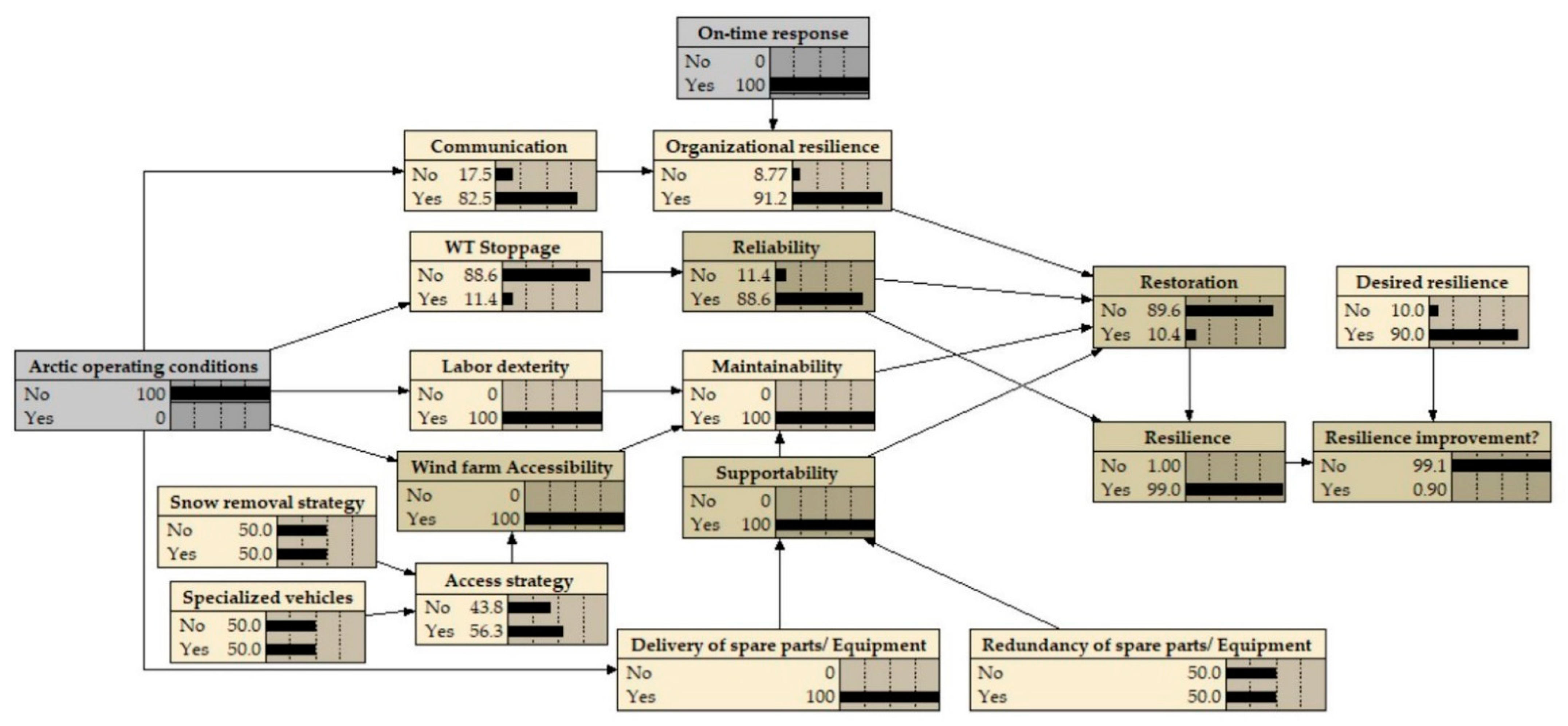
5.1. Baseline Scenario Analysis

The baseline scenario analysis concerns the resilience of the WF when it operates under normal operating conditions (no presence of Arctic disruptive events). Figure 5 illustrates the baseline scenario with the probability of occurrence of Arctic operating conditions set to 0%. Based on the available data, the resilience of the WF and the contributing factors were calculated probabilistically as follows:

Based on the gathered data, the WF experienced a total of 1993 WT stoppages during 2019. The reasons for the stoppages mainly concerned servicing and maintaining the WTs. The stoppages that resulted from Arctic operating conditions, such as icing and snow accumulations, were excluded. Based on this, the stoppage rate per WT during each month of that year was approximately 12 stoppages/WT/month. Therefore, the BN shows, by applying the Poisson distribution over the mean value of the stoppage rate (i.e., 12 stoppages/WT/month), as discussed in Equation (13), that the probability of WT stoppage is 11.4%. Consequently, the reliability of the WF, based on the BN, by utilizing Equation (4), will be 88.6% under normal operating conditions.

Labor dexterity is 100% under normal operating conditions, where the Arctic conditions are not present, which hinder the maintenance activities and limit the ability of workers to perform their work. In addition, accessibility to the WF is 100% probable since no snow has accumulated on the roads to the WF.

Regarding the supportability of the WF, the supply and provision of spare parts is 100% successful as roads are open and not affected by the Arctic conditions. Therefore, the NoisyOrDist function in Equation (16) shows that supportability is calculated to be 100% successful. Consequently, by using the NoisyAndDist function in Equation (15), it shows that the maintainability of the WF is 100% successful.

WF data show that the mean value of lost communication events between the WTs and the operator is five events per month per WT, under normal operating conditions. By applying Equation (17), the Poisson distribution over the mean value of the lost communication events shows an 82.5% probability of successful communication during non-disruptive event conditions.

In addition, by reviewing the timing and duration of the maintenance activities, it is observed that more than 85% of the maintenance procedures for failures that the WTs experience are carried out within the first hour of the failure taking place. Based on that, the on-time response is set to 100% as successful WF responsiveness. The overall organizational resilience, by applying the NoisyAndDist in Equation (18), is calculated to be successful with 91.2% probability.

By applying Equation (1) to calculate the WF resilience, the BN shows in Figure 5 that the WF is 99.1% resilient under normal operating conditions. Setting the desired resilience to be at least 90%, the resilience improvement node, which is modeled using the expression in Equation (19), in Table 1, shows that there is 99.1% no need for resilience improvement for the WF.

Table 2. Summary of baseline scenario input and output nodes.

Input Nodes	Yes Value	Output Nodes	Yes Value	Resilience
WT stoppage	11.4%	Reliability	88.6%	99%
WF accessibility	100%	Maintainability	100%
Labor dexterity	100%
Spare parts/equipment delivery	50%	Supportability	100%
Spare parts/equipment redundancy	100%
Communication	82.5%	Organizational resilience	91.2%
On-time response	100%

summarizes the values of the BN input and output nodes, and the results of a forward propagation baseline scenario that could take place, using the modeled BN shown in Figure 5.

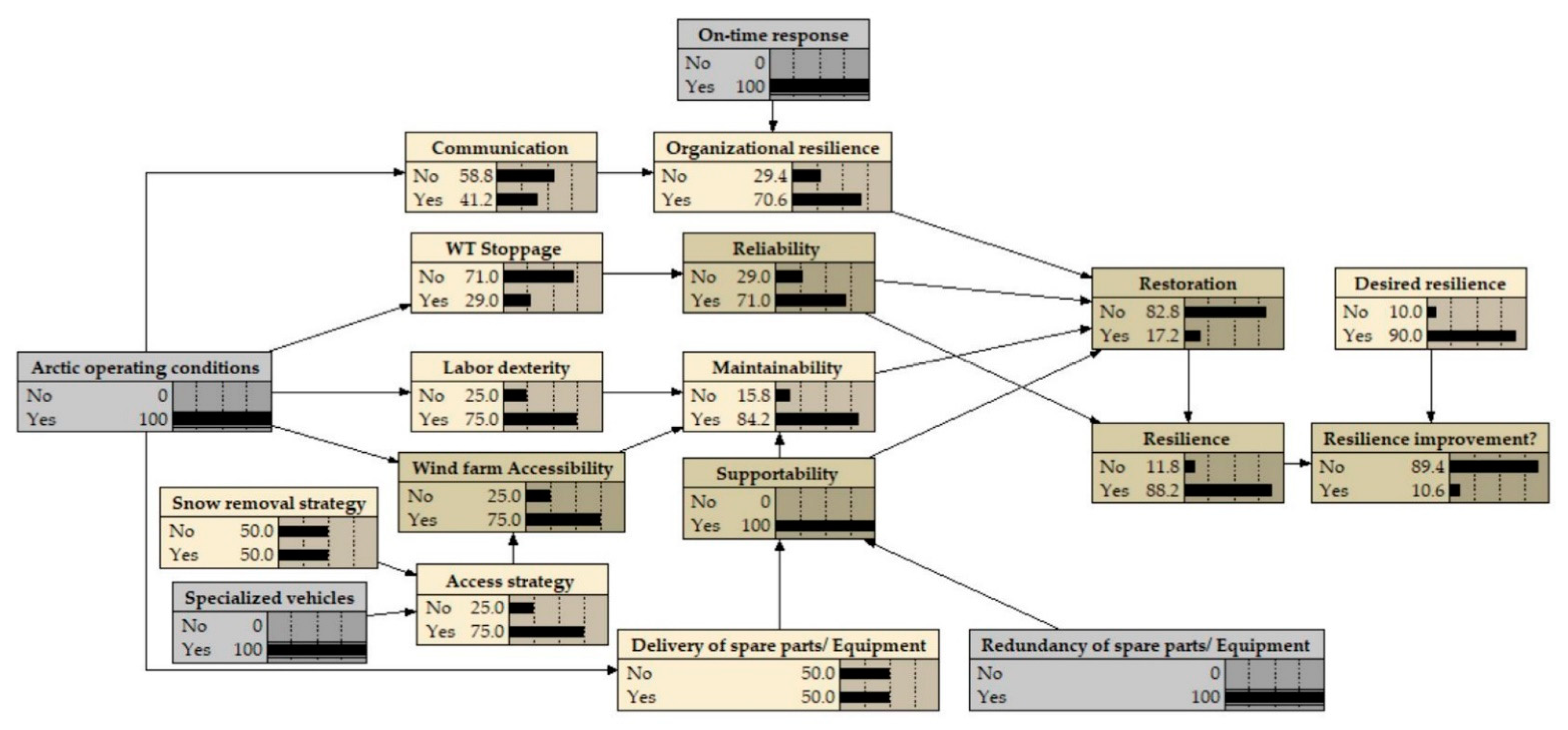
5.2. Arctic Operating Conditions Scenario Analysis

If the WF was operating under Arctic conditions, its resilience would be degraded due to the effects of ice accretion on WT blades, cold temperatures that affect the dexterity of the crew staff, and snow accumulation on roads that hinders accessibility to the WF. Figure 6 illustrates the values of the WF resilience and contributing factors. The data considered in the analysis of this scenario relate to the month of December as Arctic operating conditions are mostly witnessed during this month.

There were 65 WT stoppages altogether due to icing in December 2019. The average number of WT stoppages due to icing per WT during December is five. The resulting probability from applying Equation (13) to the average number of WT stoppages due to icing is 17.56%. By using Equation (20), the total WT stoppage probability is equal to the probability of stoppage due to icing events added to the stoppage probability calculated in the baseline scenario, under normal operating conditions, which was 11.4%. This results in 29% probability of stoppage under Arctic operating conditions. Based on that, by applying Equation (4), the calculated reliability probability is 71%.

P (WT stoppage|Arctic operating conditions) =
P (WT stoppage due to icing events) + P (WT stoppage under normal operating conditions)

(20)

The dexterity of maintenance crews during extreme Arctic conditions is assessed to be reduced by 70% due to exposure to the cold weather [28], which can lead to decreased cognitive performance, injuries, dangerously low body temperature, and loss of sensitivity. Such conditions can directly influence the uncertainty of a person’s decision or actions significantly [29]. Based on this, a simple scale can be developed to assess labor dexterity under milder Arctic conditions, such as those experienced by the WF.

Table 3. Labor dexterity success percentage according to operating conditions.

Operating Conditions	Labor Dexterity Success
Extreme Arctic conditions	0–30%
Moderate Arctic conditions	31–60%
Mild Arctic conditions	61–90%
Normal conditions	91–100%

proposes a qualitative scale for assessing the success of labor dexterity under different degrees of Arctic conditions. Labor dexterity success in the WF area during December falls within the range of 61–90%. By taking the average value of this range, the labor dexterity success would be approximately 75%.

Moreover, the WF employs a snow removal strategy to some extent, and uses specially equipped vehicles to maintain access to the WF. This can guarantee 75% successful access to the WF when applying the NoisyOrDist function in Equation (14) in the BN. By assuming that the spare parts and equipment are redundant, and available at the WF site, this would indicate 100% successful supportability, according to the NoisyOrDist function in Equation (16). This will contribute to successful maintainability of 84.2%, by applying the NoisyAndDist function in Equation (15).

According to the available data, the number of lost communication events between the WTs and the WF operator has doubled under Arctic operating conditions. In other words, the probability of successful communication between the WTs and the WF operator is halved compared to the normal operating conditions in the baseline scenario. Therefore, the probability of successful communication is reduced to 41.2%. Moreover, it is observed from the data that the responsiveness of the WF to failures did not change under Arctic conditions. Therefore, the probability of an on-time response by the operator to Arctic events remains at 100%. Based on this, the probability of organizational resilience is 70.6% when applying the NoisyAndDist function in Equation (18).

By applying Equation (3), the probability of successful restoration under the given conditions is only 17.2%. This is because the reliability of the WF is still high, even under Arctic conditions. In addition, by setting the desired resilience node to 90%, the resilience improvement node shows a slight probability of improvement urgency of 13.1%.

The resilience of the WF under Arctic operating conditions is 88.2% when calculated using Equation (1). This indicates that the Arctic conditions contributed to a 10.8% reduction in resilience, compared to the baseline scenario.

Table 4. Summary of input and output nodes in the Arctic operating conditions scenario.

Input Node	Yes Value	Output Node	Yes Value	Resilience
WT stoppage	29%	Reliability	71%	88.2%
Snow removal strategy	50%	Maintainability	84.2%
Specialized vehicles	100%
Labor dexterity	75%
Spare parts/equipment delivery	50%	Supportability	100%
Spare parts/equipment redundancy	100%
Staff communication	41.2%	Organizational resilience	70.6%
On-time response	100%

summarizes the values of the BN input and output nodes when the WF operates under Arctic conditions, using the modeled BN shown in Figure 6.

5.3. Arctic Black Swan Scenario Analysis

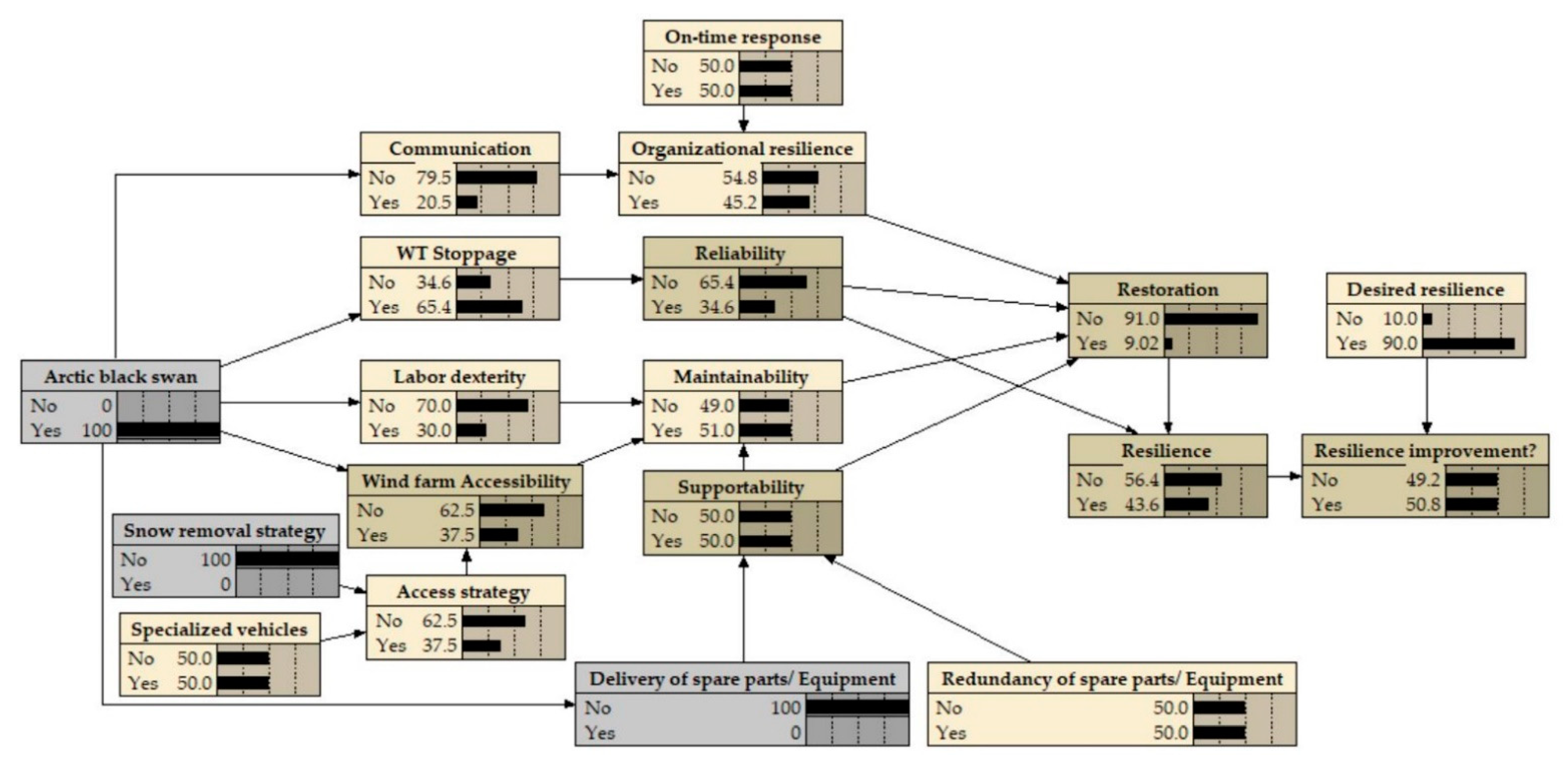
The resilience of the WF can be tested against a scenario that is unlikely to happen but which, if it were to happen, would have an immense impact on the performance of the WF. This is classified as an Arctic black swan scenario. Proposing such a scenario can help the WF operator to prepare for the worst-case scenario that the WF might face, and to consider the best measures to take in order to mitigate the impacts of such a scenario.

The imaginable Arctic black swan scenario implies a dramatic increase in the number of icing events, which are going to be 10 times the number of icing events that the WF experiences under the Arctic operating conditions scenario. Moreover, the number of lost connections between the WTs and the WF staff during this scenario would increase tenfold compared to the Arctic operating conditions scenario, and the WF’s response to such scenario events would be reduced to 50%. In addition, accessibility to the WF would be reduced as the snow removal strategy would not be efficient enough to remove the excessive accumulated snow, and only 50% of the specialized vehicles would be useable to access the WF. Lastly, the scenario suggests that roads to spare part suppliers would be blocked due to the immense amount of accumulated snow, and that only 50% of the spare parts and tools would be redundant at the WF site. Figure 7 illustrates the probabilistic values of the input and output nodes that correspond to the proposed scenario.

By following the same methodology mentioned earlier in the previous two scenarios, it can be seen from the figure that the resilience of the WF is significantly reduced to 43.6%. All resilience factors witnessed a significant reduction in this scenario, but it is the reliability of the WF that witnessed the highest reduction, as reliability is reduced to 34.6%. Moreover, due to reduced maintainability, supportability and organizational resilience, the restoration of the WF is reduced to nearly 9%. Furthermore, the improvement of the WF resilience, shown in the resilience improvement node, is increased to 50.8%, indicating a higher urgency of implementing measures to improve the resilience of the WF.

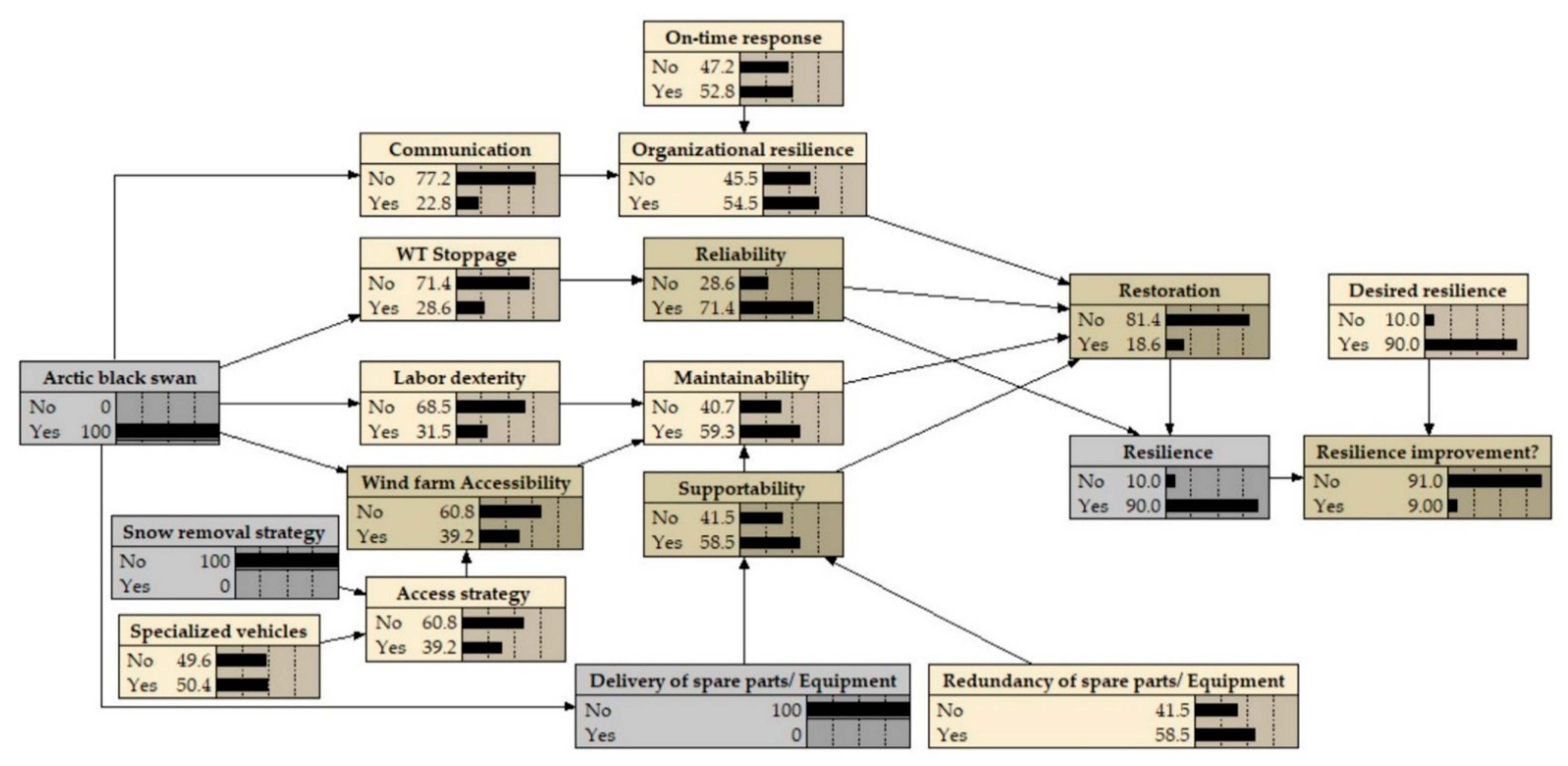
Backward Propagation Analysis

Backward propagation is another practical characteristic of BNs. In backward propagation, observation is conducted of a precise variable, usually an output variable (e.g., the resilience node or the restoration node). After that, the BN calculates the marginal probabilities of unobserved variables by introducing the impact of the observed variables into the network in a backward style. For example, if the resilience value is set at 90%, as shown in Figure 8, this scenario implies enhancing the reliability of the WF from 34.6% to 72.2%, which can be achieved, for example, by installing anti/de-icing systems on the blades of the WTs. However, a cost/benefit study should be carried out to assess the feasibility of installing such systems [30]. In addition,

Table 5. Enhancement of variables when enhancing resilience under Arctic black swan events.

Variables/Nodes	Resilience = 43.6%	Resilience = 90%
Reliability	34.6%	71.4%
Maintainability	51%	59.3%
Supportability	50%	58.5%
Organizational resilience	45.2%	54.5%

shows the required percentage value for each of the contributing factors to resilience in order to increase the overall WF resilience to 90% when operating under Arctic black swan conditions.

6. Conclusions

Infrastructure systems in the Arctic, such as wind farms, are exposed to different types of threats ranging from natural hazards to unfriendly human-induced events to accidents. Under such disruptive events, WFs need to be resilient to withstand and recover quickly and efficiently.

In this paper, resilience was probabilistically modeled using Bayesian networks. The proposed resilience model consists of variables related to the reliability, maintainability, supportability, and organizational resilience of the wind farm. The concluded resilience value is an indication of how resilient the wind farm is in the presence of Arctic disruptive events. A Bayesian network is a qualified tool for calculating prior and posterior conditional probability, through linking input and output variables in a network. Bayesian networks can be efficiently used for estimating risks and contributing to decision-making process in uncertain environments such as the Arctic region.

A WF in Arctic Norway was considered as a case study. Three separate scenarios were analyzed to calculate the WF resilience under three distinct operating conditions. The baseline scenario showed that the WF is highly resilient under normal operating conditions, with a 99% chance of being successfully resilient. The second scenario tested the resilience of the WF under Arctic operating conditions. The calculated resilience of the WF under such conditions is still high, with almost 88.2% resilience. On the other hand, the WF resilience was degraded to 43.6% under an Arctic black swan scenario. Moreover, the BN indicates that the WF needs urgent improvement actions to enhance its resilience, with a probability of nearly 51% that the WF’s resilience should be improved.

A backward propagation scenario analysis would be particularly beneficial for WF decision-makers as it provides insights into achieving a specific level of resilience. The paper illustrated the values of resilience variables in the event that decision-makers want to enhance resilience to 90% when the WF is operating under Arctic black swan conditions. The enhancement of resilience to such a level requires improving the reliability significantly by more than 25%, which can be achieved by installing anti/de-icing systems on the blades of the WTs. Regarding maintainability, supportability, and organizational resilience, the improvement range is within 10% for each of them.