A Case Study in View of Developing Predictive Models for Water Supply System Management

Abstract

Initiated by a case study to assess the effectiveness of the modernisation actions undertaken in a water supply system, some R&D activities were conducted to construct a global predictive model, based on the available operational failure and recovery data. The available operational data, regarding the water supply system, are the pipes’ diameter, failure modes, materials, functional conditions, seasonality, and the number of failures and time-to-recover intervals. The operational data are provided by the water company responsible of the supply system. A predictive global model is proposed based on the output of the operational data statistical assessment. It should assess the expected effectiveness of decisions taken in support of the modernisation and the extension plan.

1. Introduction

Within the frame of the modernisation of a regional water supply system (WSS) in Poland, an assessment of the effectiveness of the related decisions and actions was demanded by the regional authorities. The assessment of this case study was accompanied by some R&D activities to develop predictive models in support of the decision making and the management of the modernisation of the WSS.

The quality of a water supply service can be measured using different metrics. The availability and the reliability of the (WSS) are the most cited amongst these metrics. The availability measures the aptitude of the WSS to provide the water at the required quality and quantity on demand at instant “t”. The reliability measures the aptitude of the WSS to provide the water at the required quality and quantity during a period “T”. Methods of assessing the availability and the reliability of the water supply networks are well developed and widely published, among others in [1,2]. It is the same situation for case studies and WSS performance assessments [3].

Throughout the paper, the abbreviation WSS will refer to the water supply system rather than to the whole water supply service. Generally, the water supply services performance is judged upon the capacity to supply the demanded water quantity with the required pressure and the required quality (chemical-physical-biological) at the convenience of the consumers [4,5]. However, the WSS performance is just one dimension of the whole water supply service performance. For this reason, water supply utilities and other stakeholders are interested in models, methods, and standards that enable them to measure, assess, and predict the WSS availability and reliability.

The availability and the reliability are probabilistic concepts. They are not directly measurable. However, they can be indirectly measured thanks to the operational experience feedback of the WSS. The operational experience feedback provides the elementary data to develop the required predictive availability and reliability models. The WSS failure and recovery records that each water supply utility has constitute valuable sources of the elementary data needed to measure the availability and the reliability. Subsequently, water utilities put strong emphases on failure and recovery data collection, storage, and analyses within the optic of developing predictive models.

The statistical analysis of the WSS failure and recovery data permits the extraction of the failure and recovery characteristic parameters. Dependant on the nature of the collected data, the characteristic parameters can be the occurrence frequencies (failures, recoveries, etc.), the time intervals (time before failure, time before recovery, etc.), or both. Thanks to these parameters, the WSS availability and reliability can be assessed. Besides, some statistical predictive models can be developed to assess the future trends of the characteristic parameters.

The available failure and recovery data are generally impacted by technical, procedural, and managerial performance effectiveness [6]. Including all these dimensions is out of the scope of our paper, as the available data do not allow the integration of such dimensions in the assessment. So, the assessment will only consider the technical dimension.

The paper presents a case study of a given regional WSS in Poland. The objective of this case study is to assess the failure and the recovery characteristic parameters, in view of building up some predictive capabilities. The predictive capabilities are intended to support decision making in the management process of the modernisation and the extension of the regional WSS. The assessment is carried out in two phases: the statistical analysis of the operational data trends and the development of a predictive global model.

The paper describes, in Section 2, the general lines of the methodology of the study.

In Section 3, the paper presents a general description of the case study. The general description of the WSS covers the pipe-lines network: pipe types, geometrical characteristics, material specifications, and lengths in km.

In Section 3, the paper introduces the statistical assessment of both the failure database and the recovery database.

In Section 4, the predictive global model developed for the case study is proposed.

In Section 5, the paper shows the principal conclusions and findings of the assessment.

In Section 6, the paper summarises a global synthesis of the work to conclude.

2. Methodology

The background of the work is to assess the failure-recovery data of a regional WSS in Poland in view of building up first order predictive availability and reliability models. These preliminary predictive models were required to serve in predicting gross control indicators to assess the effectiveness of the decisions and the actions taken within the modernisation and the extension of a regional WSS. The developed models are preliminary as the available database is of a small size, heterogeneous, and tainted with high uncertainty level.

The case study of this WSS covered two tasks: the statistical analysis of the failure-recovery data and the development of a preliminary predictive models exploiting the outputs of the statistical analysis. Our work methodology consisted of distinguishing three spheres of activities:

• Identification and classification of the information available about the regional WSS.
• Identification of the adequate statistical analysis methods to be exploited according to the specification of the available input data and their statistical quality.
• Identification of the most adequate concepts to build up preliminary predictive models of availability and reliability, given the physical nature of the WSS and the nature of the outputs of the statistical analysis of the operational data.

The WSS specifications are given in Section 3.1. The specifications cover the extension of the WSS, the classification of the pipes, and the lengths and materials of each class of pipes. The specifications of the available failure and recovery data and time intervals covered by each dataset are determined.

The differences in nature between the available failure and recovery datasets are put in evidence. Subsequently, the choice of the adequate statistical analysis methods is done for each dataset. Both datasets were processed differently, but the main output has the same nature: an overall failure rate and an overall recovery rate.

These overall transition rates are the required outputs to build up the preliminary predictive models of the whole WSS. The details are given in Section 3.2.

Given the nature of the available output data resultant from the statistical assessment in Section 3, we had to develop a binary model considering globally two events: failure and recovery.

Given the limited amount of data, it was not conceivable to treat the WSS as a network even with limited number of nodes and edges. Subsequently, we had to opt for an overall predictive model. We had to focus on first order models as our immediate target was to obtain control indicators to assess the effectiveness of the decisions and the actions taken within the program of the modernisation and the extension of the regional WSS.

Although a global model does not allow for the description of individual segments of the network, it responds satisfactorily to the needs of assessing the effectiveness of the ongoing modernisation and the extension work in the WSS. The details about the proposed models are given in Section 4.

3. Input Data Description

The input data are distinguished in two classes: network descriptive characteristics and operational feedback failure-frequency and recovery-time data.

Network descriptive characteristics cover the following groups:

• General information about the objects (locations, ages, etc.).
• Technical data about the objects (types of objects considering their functionality, geometry, materials, technology, operational conditions, etc.).
• Data on failure (type of event, cause, mechanisms, etc.).
• Data on the effects and consequences of failure (type, damage severity, extensions, etc.).
• Additional information (report date, environmental data, cost).

The operational feedback failure-frequency and recovery-time data is presented in two independent databases with two different structures: the failure-frequency database and the recovery-time database. The structural differences between the two databases may be the result of the separation between the operational surveillance task and the maintenance task due to some local organisational conditions.

The data type is different from one database to the other. In the failure database, one counts number of failures per given time-interval while one measures intervals of time-to-recover in the recovery database. Both measurables are random but different in nature.

Regarding the scope of the paper, the final outcomes we are looking for are an “overall failure rate” and an “overall recovery rate” to globally characterise the WSS. They may be called “global failure rate” and “global recovery rate” as well. They are sometimes called system equivalent parameters [7], especially if they are calculated based on the characteristic parameters of the system’s constituents. These global characteristic parameters are necessary to assess the quality of the water supply service, to support the decision making regarding the modernisation of the WSS, and to develop global predictive models of availability and reliability.

The global characteristic parameters will then be designated as:

• The overall failure rate of the WSS, ${\lambda }_{WSS}$.
• The overall recovery rate of the WSS, ${\mu }_{WSS}$.

It is important to underline that the estimated characteristic parameters (${\lambda }_{WSS}$, ${\mu }_{WSS}$) are describing the global functional behaviour of the WSS. They cannot be used to characterise a zonal portion of the WSS, a single type of the pipes (main, distribution, connection), or for maintenance optimisation purposes. However, they are useful in automatic monitoring of event occurrences in the network. The predictive models that we are looking for are global. These are point-like models.

3.1. Network General Description

The analysed water supply network is a ring system formed by four mains with the total length of about 50 km. The total length of the water pipes including the mains is about 900 km. Distributional pipes represent ~60% of the total length of the pipes, the length of the water supply connections represents ~35%, and the mains represent only ~5% with a length increasing rate of about 1.3% in comparison to the total length of the network, in the last year of the analysis.

The pipes made from:

• Polyethylene (PE) represent 32% (289.5 km) of the total length of the water pipes.
• Polyvinyl chloride (PVC) pipes represent 28% (254.6 km).
• Galvanized steel (GS) pipes represent 24% (213.6 km).
• Cast iron (CI) pipes represent 11% (103 km).
• While those from hard steel (HS) represent about 3% (30.6 km), and the ductile iron (DI) pipes represent less than one percent (~10 km).

During the last decade, the pipes made from PE and PVC are increasingly used.

The age distribution of the mains and the distributional network is:

• Pipes aged less than 10 years represent 31.2% of the total operating water pipes.
• Between 11 and 25 years represent 23.2%.
• Between 26 and 50 years represent 31.8%.
• Above 50 years represent 13.8%.

The share of the pipes aged less than 10 years is gradually increasing due to the replacement of the damaged pipes and the renewing activities following the expansion of the city districts and the creation of new settlements. To ensure better control on the network operational performance, the water company manages the network through monitoring and recording pressure and flow rate, in the first and second zones.

3.2. Failure Data Assessment

Failures are generally classified by cause, mechanism, and/or criticality. Root causes can be of different origins such as: design, construction, and/or operational conditions [8,9,10,11,12]. Failure analysis activities are very impacting on network everyday operational and maintenance decision making [13,14].

However, the failure database we have is limited. Its failure records contain only the number of failures per month in the network, over 18 years. The failures are classified by the pipe’s position, geometry, material, and type (main, distribution, connection). No direct data were available regarding the “time to fail” per month per segment of pipe. Information about failure causes or criticality are almost absent, inconsistent, or incomplete.

The assessment aims at the determination of an overall failure occurrences trend in the network considering the field operational reality and the continuous expansion of the network due to the expansion of the town itself and the modernisation of the WSS. The failure data cover eighteen years of operation.

Given the small size of samples per class of failures, we had to work out an overall failure rate, mixing failure data over all ages, failure causes, modes, mechanisms, and criticality. We kept only the functional classification: distribution, connection, and main. As it is an overall failure occurrence rate and given the heterogeneity, it cannot be used for maintenance or for safety purposes. It just counts failures occurrences.

Data quality analysis was mainly related to the correction of errors through the use of control assumptions checking arithmetic and logical relations among statistical data, their completeness, and their accuracy. In water supply practice, the collected data may be burdened with random errors, which results from mistakes in their collection and processing and systematic errors; therefore, to assess the credibility of data, it is necessary to perform substantive and formal verification of their truthfulness, which consists of random checking of reliability, comparing the consistency of related data and plotting data graphs.

Given the dataset we have, different failure analysis models and methodologies are possible: the cumulative failure distributions [15,16], the data-driven modelling techniques using neural network and neuro-fuzzy methods [17,18], the Weibull-exponential failure model and the constant probability replacement model [19], the probability of main failure method [20], or the polynomial regression methods.

The available failure database contains the number of failures per month. So, failure rates can be directly estimated using polynomial regression techniques, based on the number of failures of all pipes within a given sampling interval [1,2,6]. The choice of the unit sampling interval is important to guarantee an acceptable statistical quality of the estimated failure rate. The notion of “Guarantee” in probabilistic analyses is generally replaced by a statistical meaningful term which is “the statistical quality”. Regarding the regression and data fitting, the “statistical quality” is assessed using indicators such as: the variance, the most likelihood probability, and/or the least-square values. In our polynomial regression, we used the R-Squared indicator.

Some preliminary investigations were carried out using different sampling intervals: 1, 3, 6, and 12 months. The sampling interval of one year was selected as it showed an acceptable dispersion behaviour in terms of variance and suits the engineering use of the water sector.

3.2.1. Failure Data Regression Processing

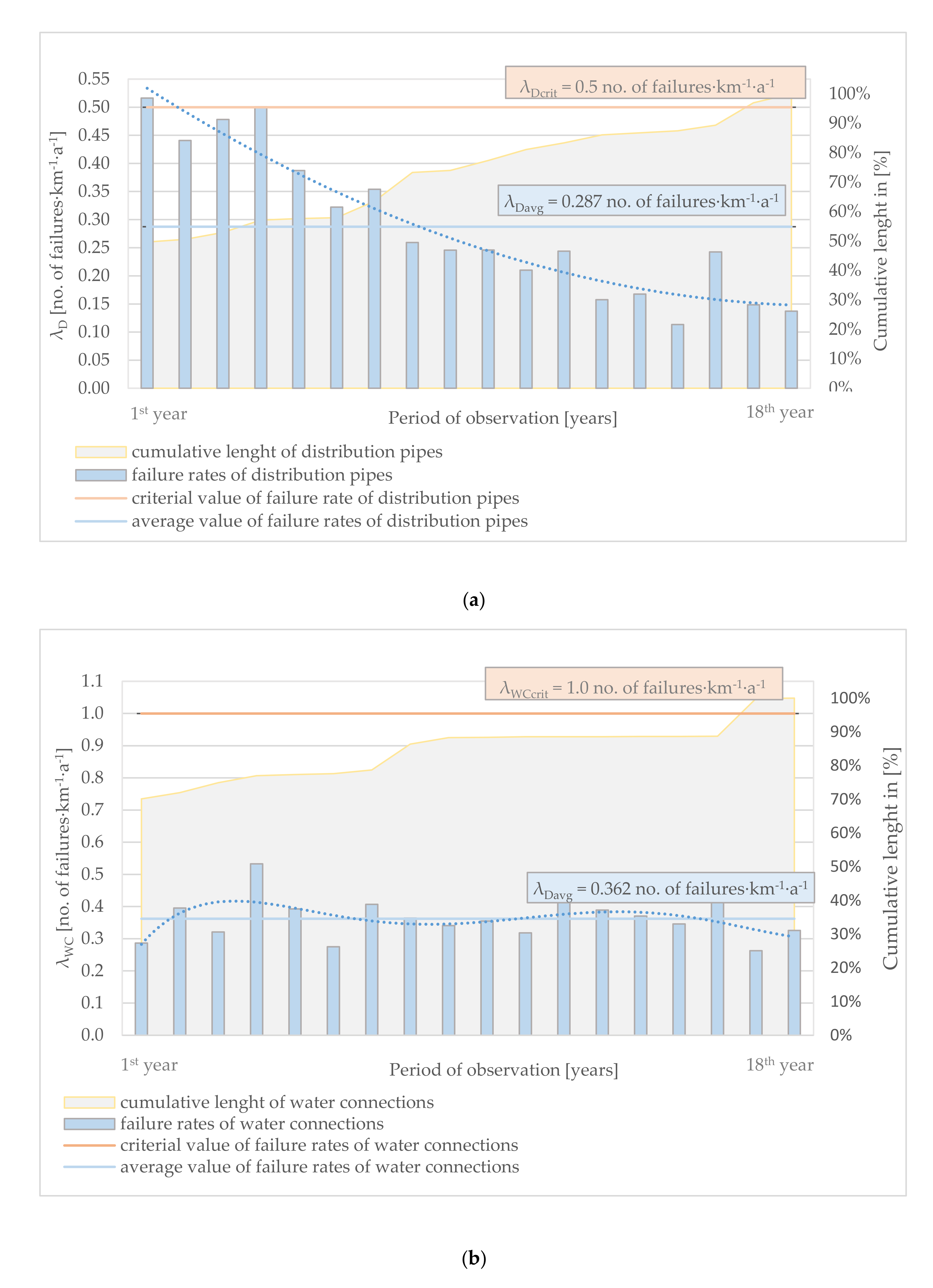
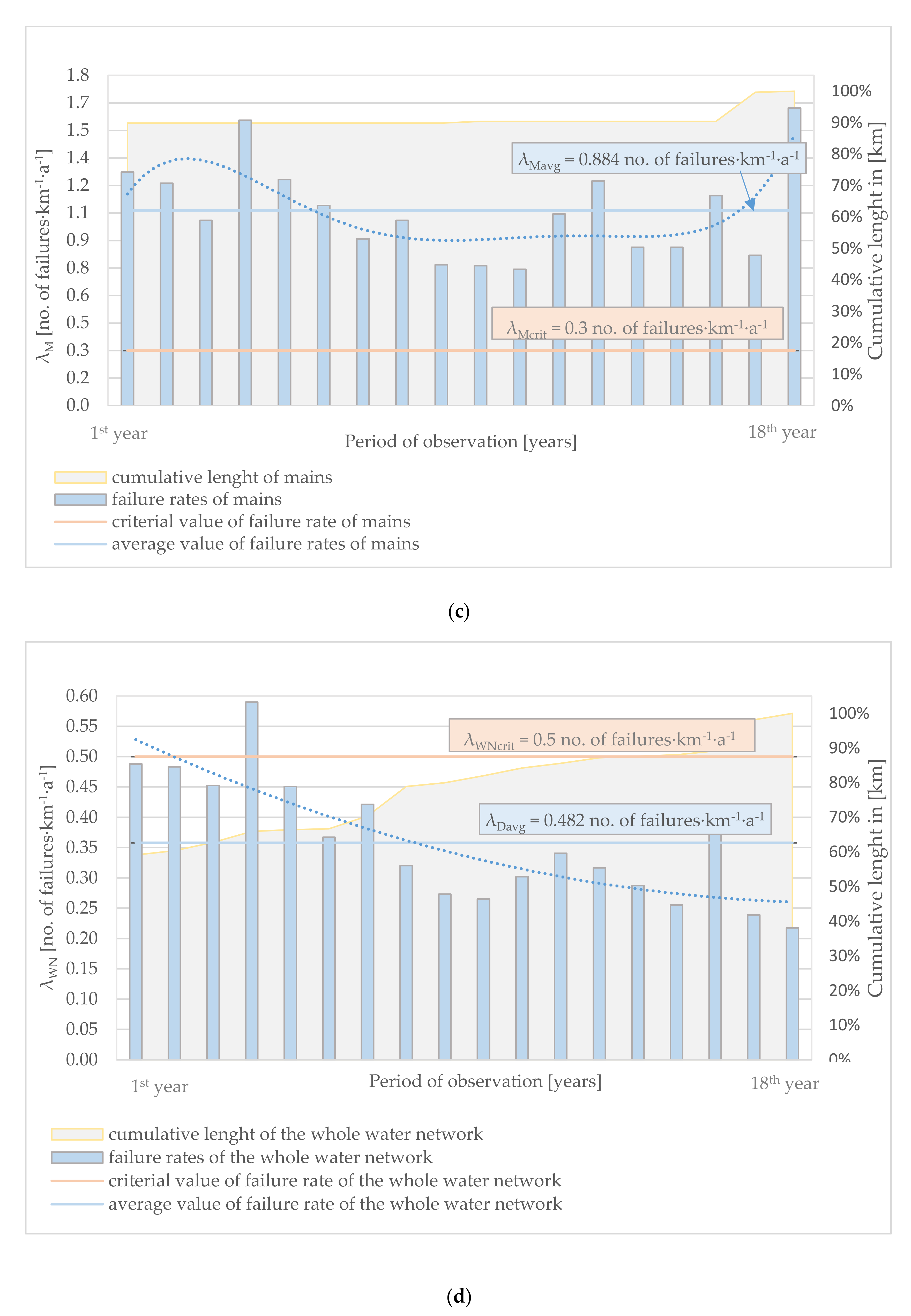
Both linear and polynomial regressions were performed. Then, we only considered the polynomial regression of order $n\ge 2$ when it gives higher statistical quality based on the R-Squared ($R^2$) value, otherwise the average values are considered. This is the case with the distribution pipes failure rate in Figure 1a and the overall failure rate in Figure 1d where the 2nd order polynomial regression results were considered. Otherwise, the average values are considered for the connections, Figure 1b, and the mains, Figure 1c.

We recall that the overall failure rate is a global measure as it covers all pipes of all types, all ages, all geometries, and all materials, independently of the zonal variation.

The annual failure data of the distribution-pipes are traced over 18 years, Figure 1a. The average failure rate is accordingly $2.87\times {10}^{-1}no.offailures·k{m}^{-1}·a^{-1}$. The polynomial regression estimates that the distribution-pipes failure rate can be determined by the following 2nd order polynomial equation, with $R^2=91\%$:

$${\lambda }_{dis}=0.0012t^2-0.0452t+0.5777,$$

(1)

where $t$ is given in years.

The R-squared value of $91\%$ indicates that the estimated polynomial is statistically of a good quality and can satisfactorily represent the variations of the distribution-pipes with the time within the vicinity of 18 year-interval.

The annual failure data of the connection-pipes are traced in Figure 1b. The best estimated polynomial regression is found to be a polynomial of 5th order with $R^2=27.8\%$, as following:

$${\lambda }_{con}=7\times {10}^{-6}{t}^5+\mathrm{f}4\times {10}^{-4}{t}^4-0.007t^3+0.0675t^2+0.009t+0.0194,$$

(2)

Given the low value of $R^2$, the polynomial was rejected, and the average value of the failure rate is considered as representative of the connection-pipes failure trend in the vicinity of the 18 years, such as:

$${\overline{\lambda }}_{con}=3.62\times {10}^{-1}no.offailures·k{m}^{-1}·a^{-1}$$

Similarly, the annual failure data of the main-pipes are traced in Figure 1c. The best estimated polynomial regression is found to be a polynomial of 5th order with $R^2=49\%$, as following:

$${\lambda }_{mai}=3\times {10}^{-5}{t}^5-0.0015t^4+0.0265t^3-0.2085t^2+0.6351t+0.7024,$$

(3)

Given the low value of $R^2$, the polynomial was rejected, and the average value of the failure rate is considered as representative of the main-pipes failure trend in the vicinity of the 18 years, such as:

$${\overline{\lambda }}_{mai}=1.06no.offailures·k{m}^{-1}·a^{-1}$$

It is worth mentioning that despite the low statistical quality of the failure data of the connections and the mains, their impact on the WSS overall failure is relatively minor as they represent less than 35% of the whole WSS pipes’ length. This is confirmed by the following.

The overall failure rate trend in Figure 1d shows a similar trend pattern as the distribution-pipes one in Figure 1a. The overall annual failure data of the WSS are traced over 18 years, Figure 2d. The average failure rate is accordingly $4.82\times {10}^{-1}no.offailures·k{m}^{-1}·a^{-1}$. The polynomial regression estimation with the 2nd order polynomial, with $R^2=70.3\%$, is:

$${\lambda }_{tot}=0.0008t^2-0.0309t+0.558,$$

(4)

The R-squared value $R^2=70.3\%$ indicates that the estimated polynomial has an acceptable quality and can statistically represent the global failure trend of the WSS pipes around the vicinity of 18 years.

The numerical results of the statistical assessment are synthesised in

Table 1. Synthesis of the statistical analyses of the failure data.

Pipes Type	Average $\mathit{N}\mathit{o}.\mathit{o}\mathit{f}\mathit{F}\mathit{a}\mathit{i}\mathit{l}\mathit{u}\mathit{r}\mathit{e}\mathit{s}\mathbf{·}\mathit{k}{\mathit{m}}^{-1}\mathbf{·}{\mathit{a}}^{-1}$	Estimated Trend	${\mathit{R}}^2$	Relative Length
Distribution	$2.87\times {10}^{-1}$	${\lambda }_{dis}=0.0012t^2-0.0452t+0.5777$	$91\%$	~60%
Connections	$3.62\times {10}^{-1}$	${\lambda }_{con}=7\times {10}^{-6}{t}^5+4\times {10}^{-4}{t}^4-0.007t^3+0.0675t^2+0.009t+0.0194$	$27.8\%$	~35%
Mains	$1.06$	${\lambda }_{mai}=3\times {10}^{-5}{t}^5-0.0015t^4+0.0265t^3-0.2085t^2+0.6351t+0.7024$	$49\%$	~5%
Total	$4.82\times {10}^{-1}$	${\lambda }_{tot}=0.0008t^2-0.0309t+0.558$	$70.3\%$	~100%

. It would be useful to recall that R-squared $R^2$ was the only control criteria used to select the polynomial regression models. We considered that a polynomial regression model with $R^2>70\%$ would be acceptable for a polynomial order $n\le 6$. The control coupled-criteria ($R^2,n$) is arbitrary and justified by a good applied statistics expert judgement. Investigating more advanced analysis techniques such as Fourier decomposition or stepwise regression were not justified given the small size of the dataset, the strong heterogeneity of the data, and its low statistical quality.

It can be noted that the average value of the annual failure rate in the mains ($1.06no.offailures·k{m}^{-1}·a^{-1}$) significantly exceeds the recommended value for the mains, which should be less than $0.3no.offailures·k{m}^{-1}·a^{-1}$ [21]. The average values of the distribution-pipes and the connection-pipes failure rates do not exceed the recommended values given in the literature [21,22].

As we are interested in predicting the failure behaviour of the WSS after the 18 years of measures, we are then interested in the overall failure rate ${\lambda }_{WSS}$ in the vicinity of the 18 years.

Considering the time behaviour of the WSS overall failure rate given in Figure 1d, one can estimate the WSS characteristic overall failure rate in the vicinity of the 18th year ${\lambda }_{wss}=0.25\times 900=2.25\times {10}^2{a}^{-1}\approx 18.8m^{-1}\approx 6.3\times {10}^{-1}{d}^{-1}$. This figure will be used in the global predictive models later.

3.2.2. Seasonality Analysis

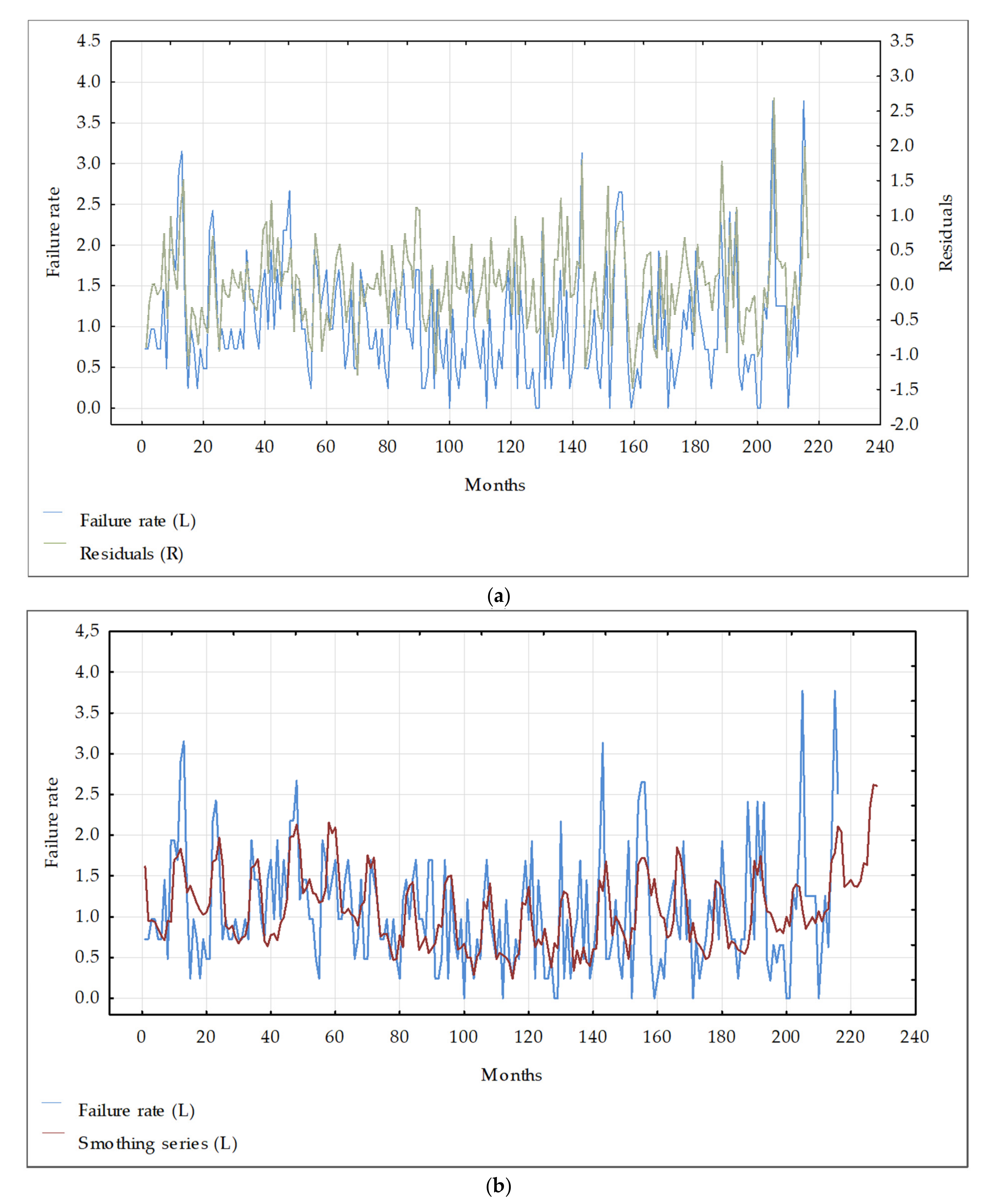
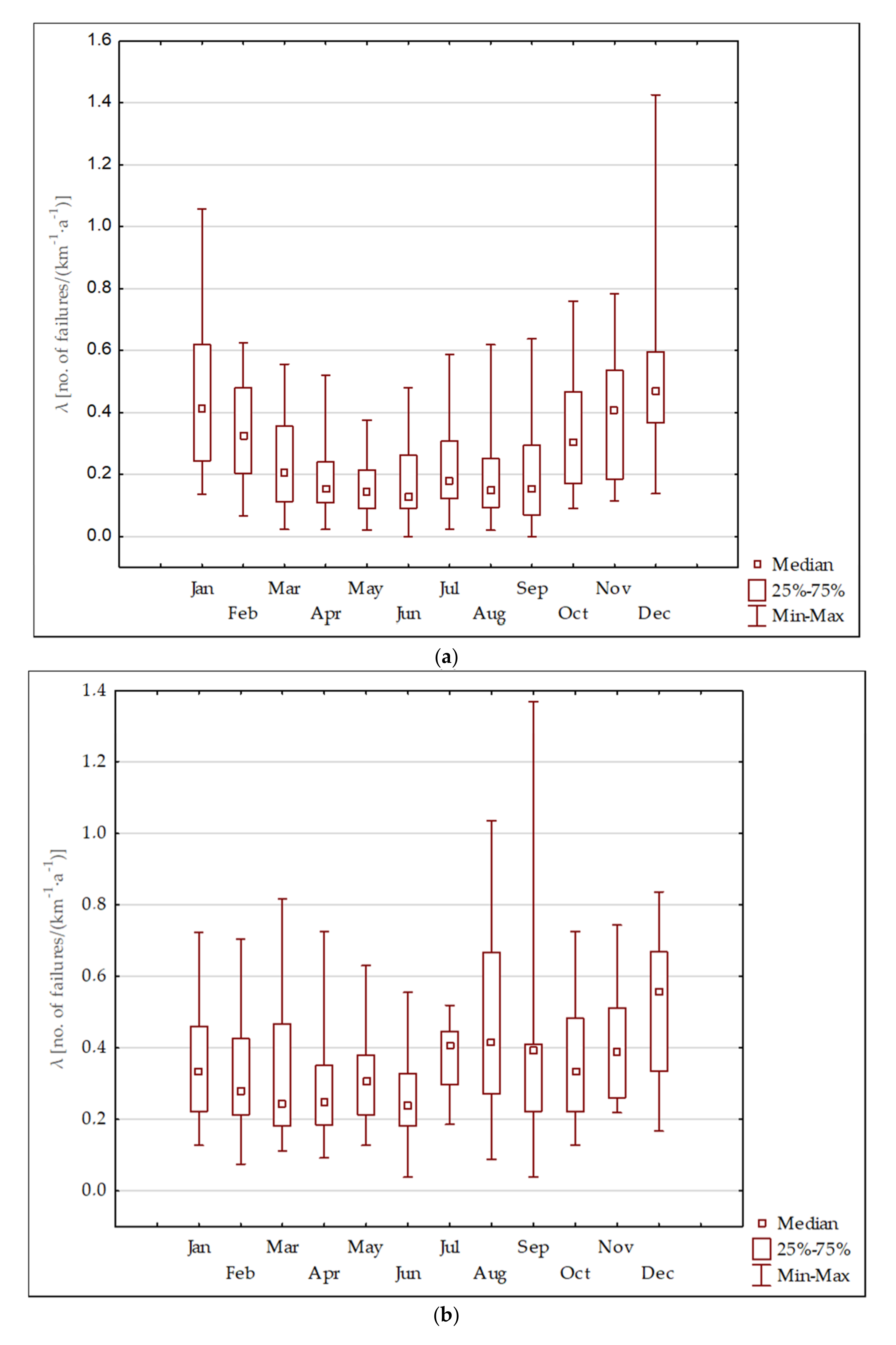
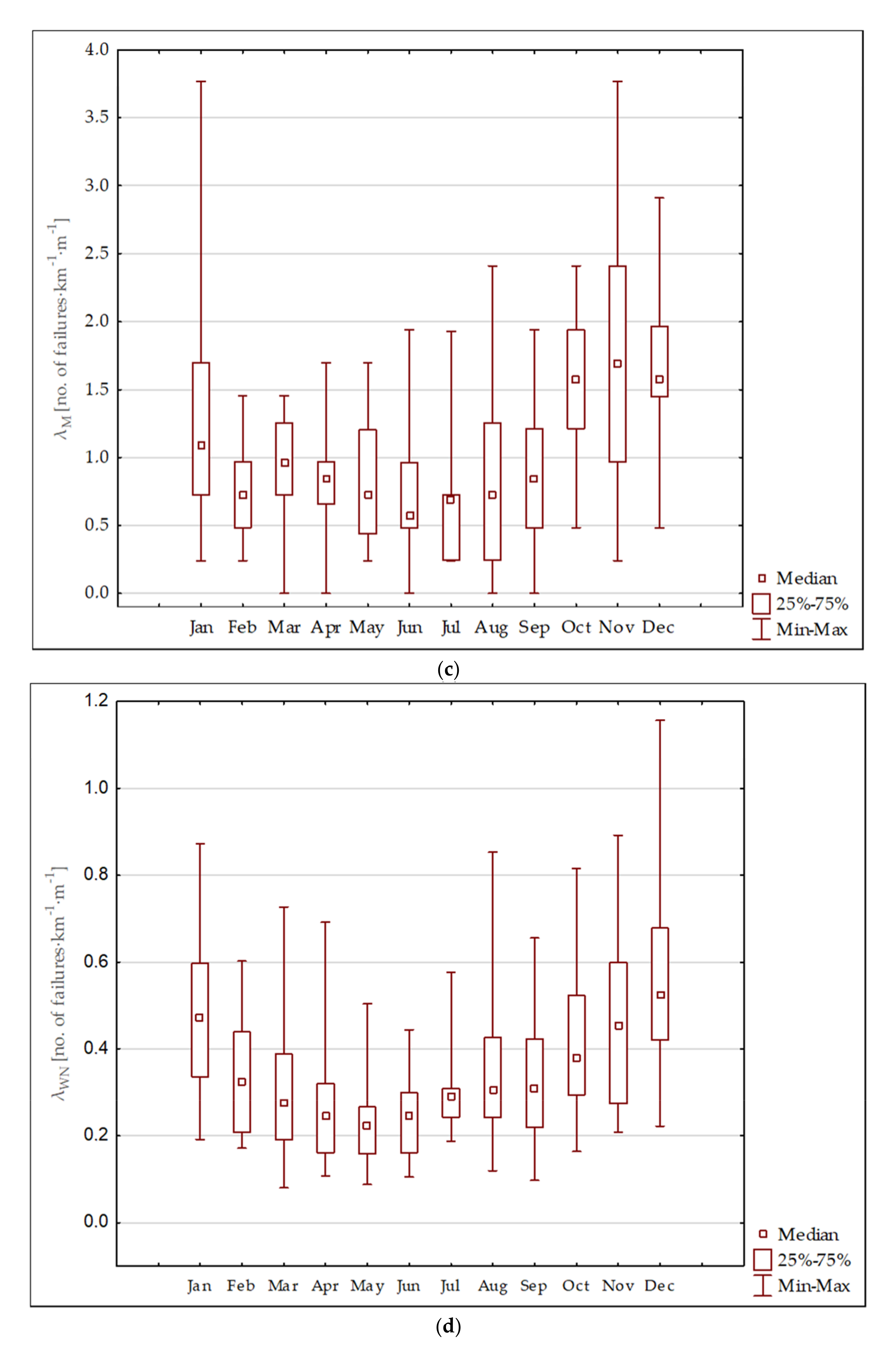
The impact of the seasonality on the WSS failures has also been assessed using Statsoft [23]. Statsoft software exploits, amongst others, the autoregressive integrated moving average (ARIMA) model [24]. A preliminary analysis of the data inherent variance was conducted, so as to verify the significant differences between months (Figure 2).

It is necessary to recall that the most significant statistical seasonal impact is on the mains (Figure 2). The seasonal impact is much less significant on the overall failure rate as the contribution of the mains in terms of km is less than 5% of the total WSS 900 km.

The parameters of the ARIMA model (p = 1, d = 0, q = 0) are assumed based on the autocorrelation graphs, using the so-called Box–Jenkins approach [24], where: p is the number of autoregressive terms, d is the number of differences, and q is the number of moving averages. This is the first order ARIMA model. Using higher orders of ARIMA models or more complex Fourier decomposition analyses were justified neither by the statistical quality of the data nor by the low seasonality effect. We recall that we have only failure occurrences per month in our database, with no additional information neither about failure modes nor about failure criticality.

The basis of the implemented approach is presented among others in [24,25]. The analysis of the average failure rate (per month) indicates that the failure culmination occurred is in December (at p = 0.00251, with current effect F (11.33) = 3.5081).

Figure 3 presents main-pipes failure rate changeability with combinations of the last observations and previous predictions adjusted for seasonal fluctuations.

For the connections, the series is more stationary regarding the ARIMA model. Only the autoregression of the first order is important, the Holt-Winters model is well matched without the trend but with the seasonality. For the failure rate of the distribution pipes, a seasonal downward trend is observed. That can be particularly observed in the Holt-Winters model with a trend that seems slightly better estimated than in the ARIMA model.

Annual seasonality and autocorrelation can be worked out for the entire network. This is evidenced by the statistically significant coefficients of “normal”. The seasonal autoregression in the ARIMA model is in accord with the Holt-Winters model [25], without the trend but with the seasonal component.

The basis of the implemented approach is presented among others in [24,25]. The Holt–Winters exponential smoothing is a statistical forecasting method in time series univariate methods. Exponential smoothing models and auto regressive moving average model proved to be the most adapted to assess temperature seasonality in many comparative assessments such as in [26,27]. The statistical fundamentals are clearly exposed and applied in [28].

3.2.3. Temperature Impact on the WSS Failures Behaviour

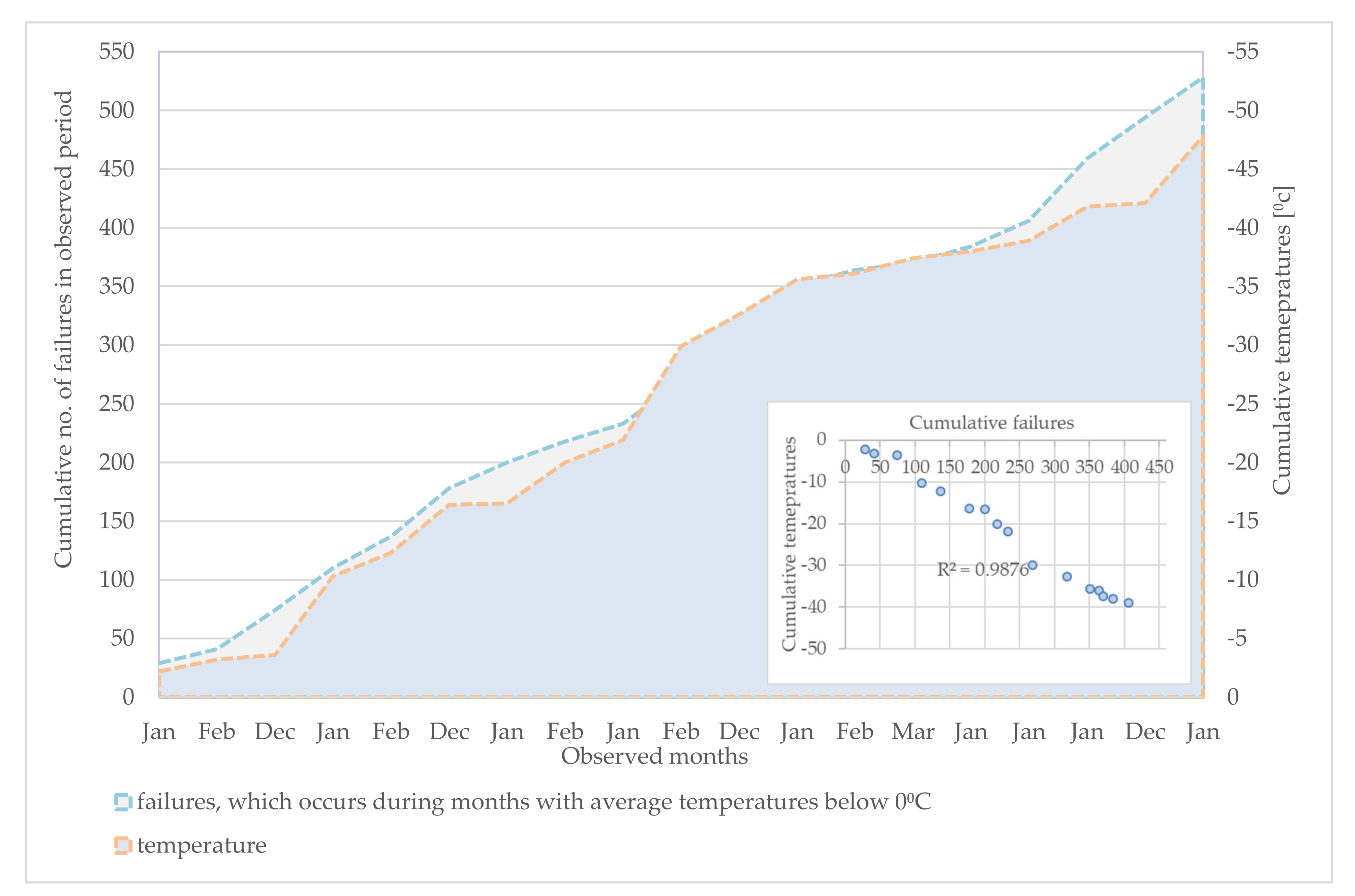
Regarding the meteorological parameters, we observed that low temperatures increase both the failure frequency of water pipes and the recovery times. The high correlation of dependence between the cumulative failures and the months with temperatures below zero Celsius are shown in Figure 4.

3.3. Recovery Data Assessment

The recovery database records contain the component-repair time and the organisational-repair time for each recovery event. Being the sum of the component-repair time and the organisational repair time, the recovery times are classified by failure mode and pipe’s geometry, material, and type (main, distribution, connection).

The assessment aims at the determination of the global recovery trends of the network considering the field operational reality, the continuous expansion of the network, and the modernisation of the WSS. The recovery data cover ten years of operation.

Recovery can generally be classified according to: the failure mode [22], the operational conditions [29,30], the location [31], the logistic conditions [32,33], and/or the managerial context [34,35]. The recovery times and the effective repair times analysis methodologies are well developed and published as well [36,37,38,39].

Regarding the recovery database we have, it contains only time intervals in two classes: physical component-repair times and associated organisational times, over 10 years. There is no additional information in the dataset. The recovery data are measured in time-intervals, not in repair frequencies, as in the case of failure data above.

Then, the data is grouped by subclasses: annual, failure mode, pipe material, pipe diameter, and pipe type (connection, distribution, main).

We will precisely be interested in analysing the component-repair time ($T_c$) and the organisation-repair time ($T_o$) within the intention to estimate the WSS overall recovery-time, ($T_r$). We recall that the recovery time ($T_r$) is the sum of the component-repair time ($T_c$) and the organizational-repair time ($T_o$).

The WSS recovery time is generally impacted by many factors. The following factors are considered in the assessment: the maintenance process, pipes material and diameter, failure modes, seasonal variations, and the average atmospheric conditions.

3.3.1. Maintenance Process Impacts on the Recovery Time

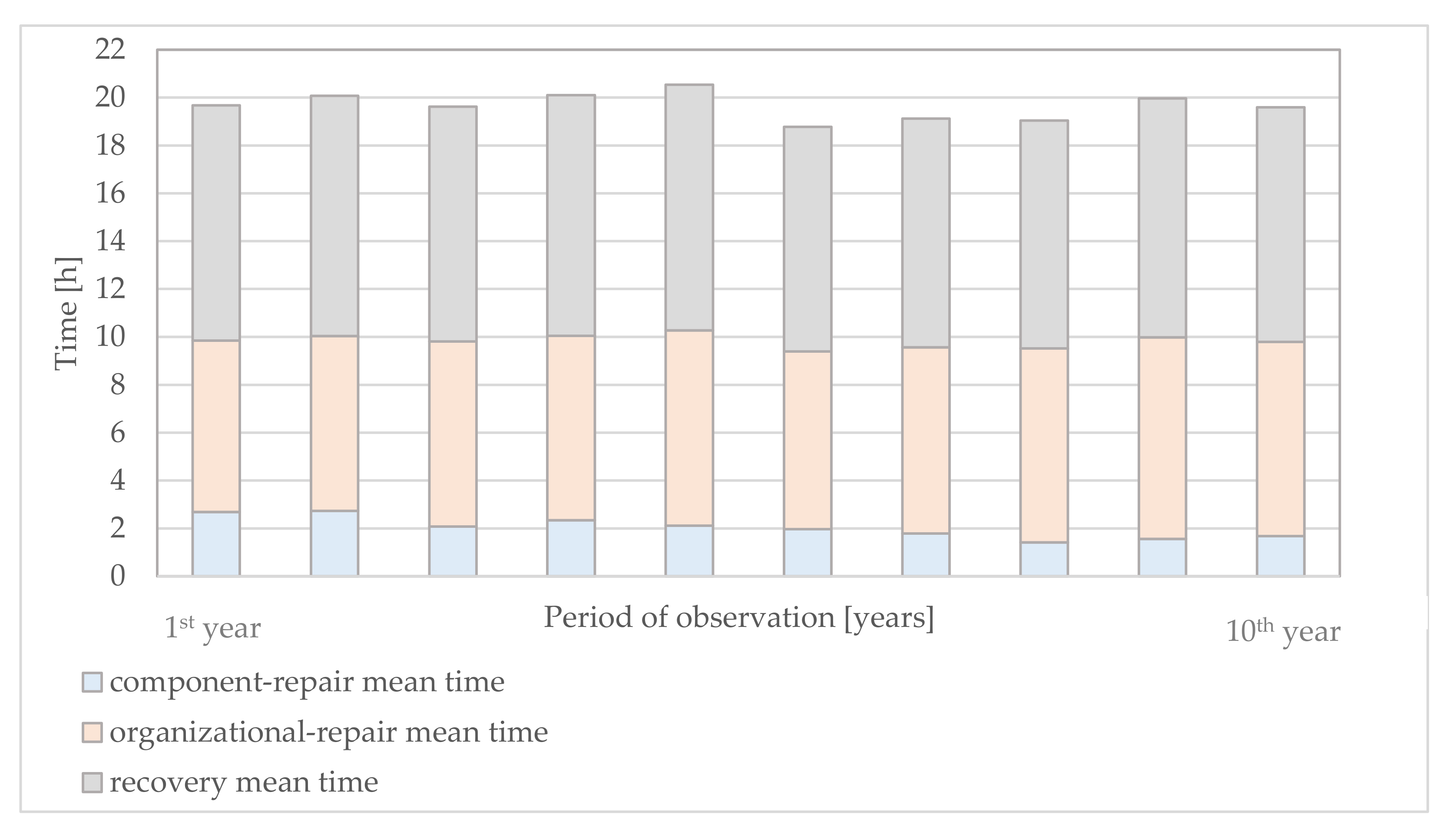
In Figure 5, the meantime of component-repair ($T_c$), the meantime of organizational-repair ($T_o$), and the recovery meantime ($T_r$) are shown.

Two observations can be stated:

• The organisational meantime $T_o$ is significantly longer than the component-repair meantime $T_c$ by factor ~3.
• The variability per year in the component-repair meantime $T_c$ is much more significant than in the organisational-repair meantime $T_o$.

The resultant annual recovery meantime $T_r$ is mainly driven by the organisational and administrative characteristic of the maintenance activities and shows a weak variability over the monitored period of 10 years. The recovery meantime $T_r$ is estimated to be about $9.8\mathrm{h}$ per reparation intervention, averaged over the 10 years (

Table 2. The recovery times’ mean values.

Parameter	${\mathit{T}}_{\mathit{c}}$	${\mathit{T}}_{\mathit{o}}$	${\mathit{T}}_{\mathit{r}}$
Meantime—µ (h)	2.04	7.79	9.83
σ	0.45	0.41	0.27
σ/µ%	22.04%	5.27%	2.78%
Upper limit	2.73	8.42	10.27
Lower limit	1.42	7.15	9.39

).

3.3.2. The Recovery Time vs. the Pipe Type

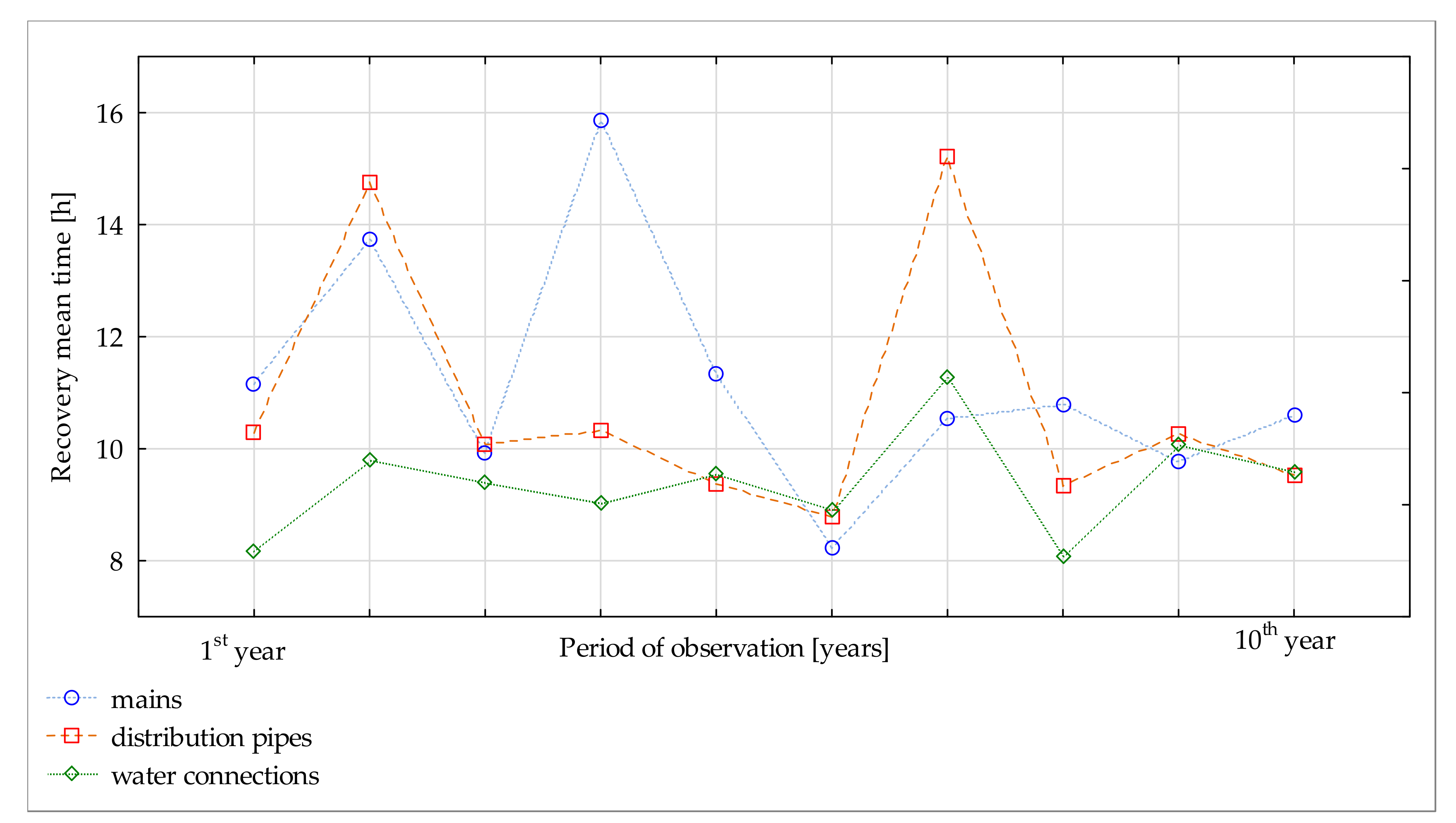
The analysis of the factors influencing the recovery time started by classifying the pipes as: mains, distributional, and the connections. The three classes are distinguished by their size, i.e., diameters.

Figure 6 presents the annual recovery meantime per class of pipes.

Regarding the recovery meantime, we counted: for the mains (766 recovery samples within the considered period), for the distributional pipes (1928 recovery samples), and for the water connections (1576 recovery samples). The recovery meantime is 8.76 h in the mains, 7.67 h for the connections, and 7.85 h for the distributional pipes. The longest recovery meantime was 33 h for the distributional pipes. The approximate values of the recovery meantime in various water pipes are driven by the priority of repairs given to the mains and the longer repair time due to the materials and dimensions of the pipes. The analysis in function of the diameters showed shorter recovery meantime in the case of the connections compared to the pipes of larger diameter. Shorter recovery meantime is observed in the water connections due to the higher accessibility to the failure location, the smaller diameter, and the types of materials.

3.3.3. The Recovery Meantime vs. Pipe Material

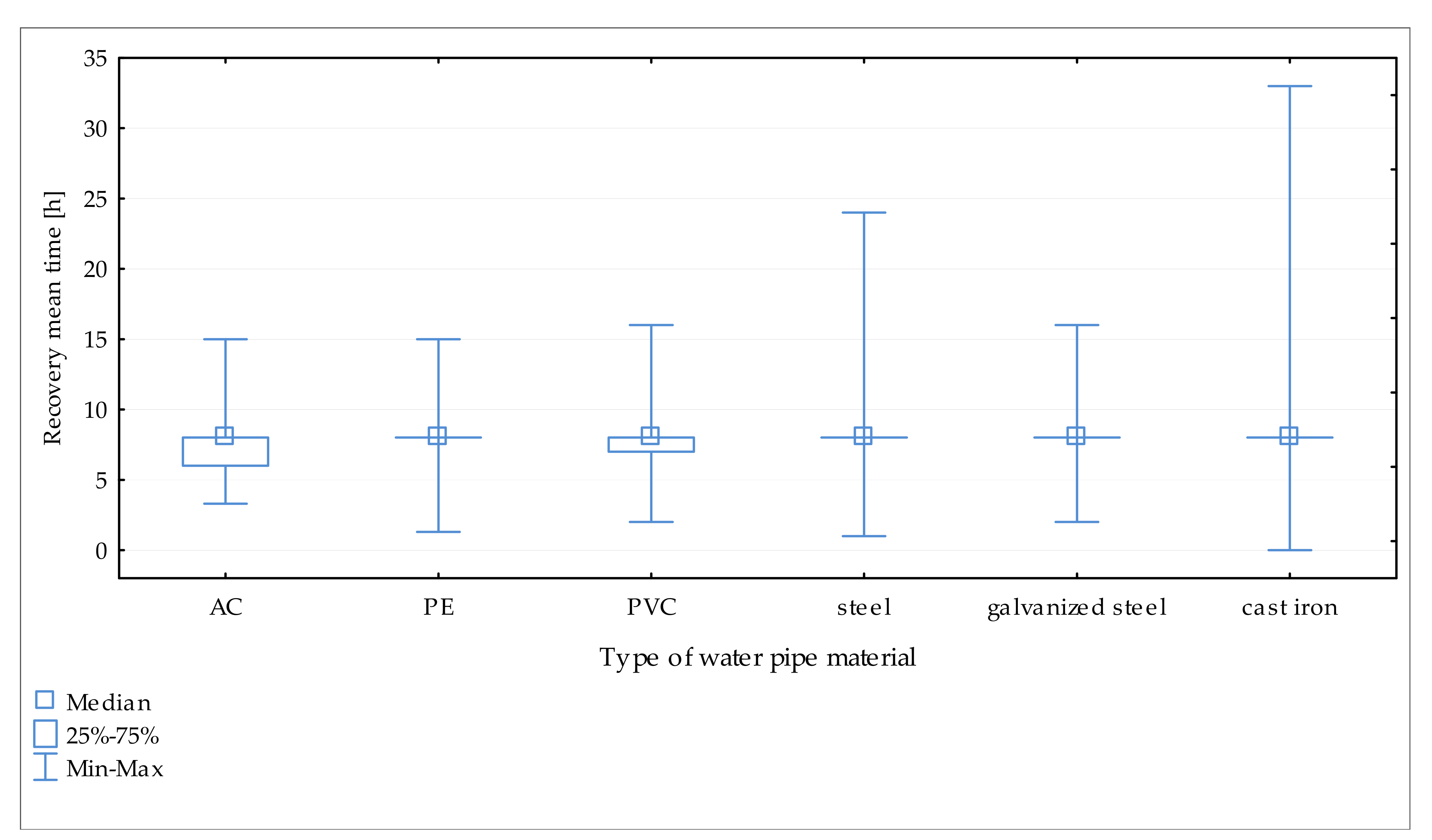
The impact of the pipes’ material on the recovery meantime is shown in Figure 7.

The longest recovery meantime was recorded for the pipes made of grey cast iron. In addition, a long recovery meantime was observed for steel and asbestos-cement pipes, which were used to build water supply systems in the last century. For grey cast iron the maximum observed recovery meantime is 33 h vs. 24 h for steel.

In the case of other materials and plastics, which are currently used on a large scale in the construction of the water supply network, the recovery meantime is less than 16 h. For plastic materials, repairs are easier and do not require the mobilization of heavy special equipment.

3.3.4. The Recovery Meantime vs. Failure Mode

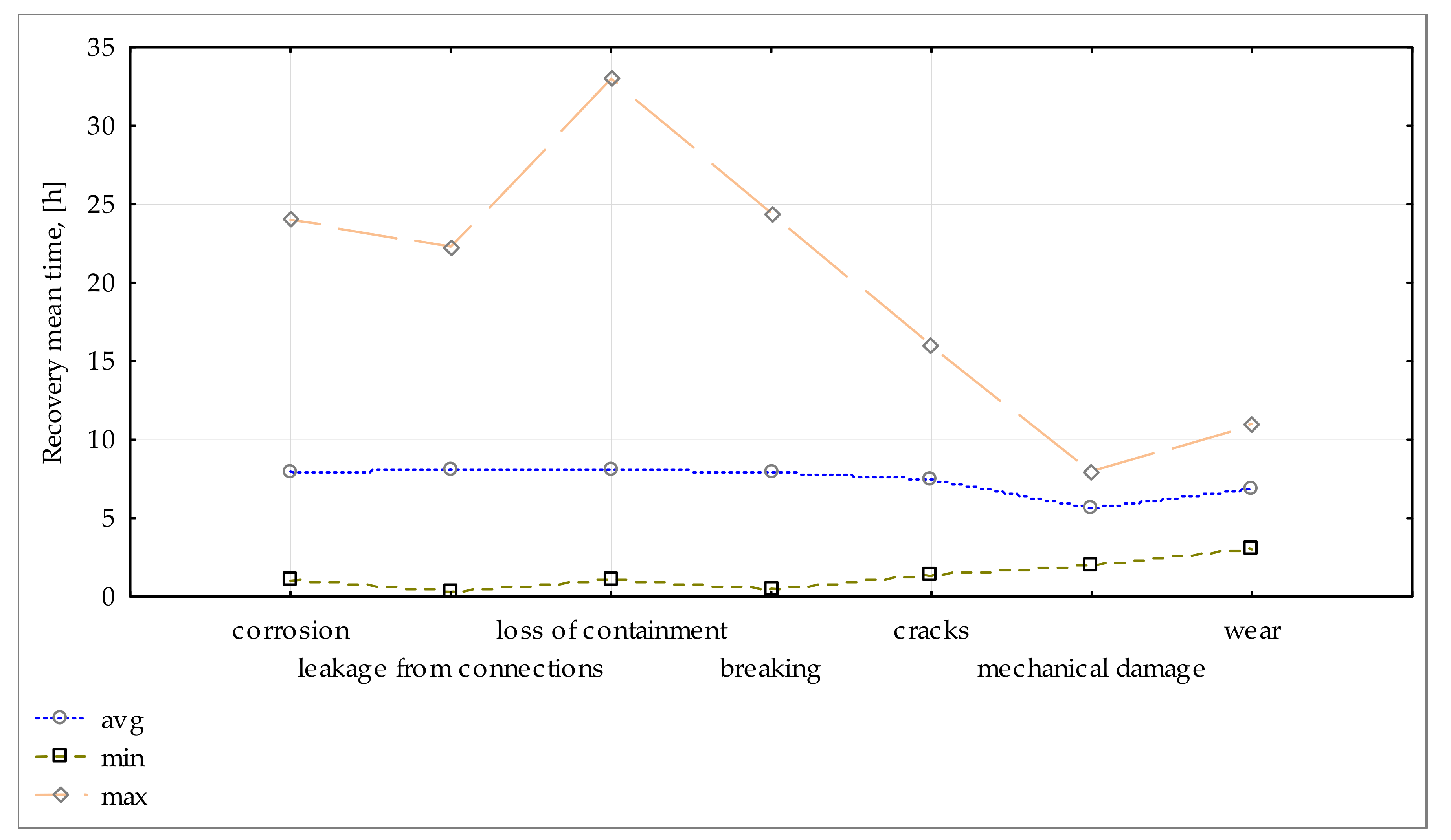
Another important factor determining the recovery meantime is the failure mode. Figure 8 presents the recovery meantime per failure mode over ten years.

It can then be stated that the shortest recovery time occurred for mechanically damaged pipes, amounting on average to 5.63 h. This mode of failures is due to earthworks. The shorter recovery meantime is explained by the faster failure location process. The longest recovery meantime occurred in pipes on which sealing is lost or pipe breaking occurred. It may reach in many cases the maximum value of 16 h. This can be explained by the pipe damage degree, the difficulty of failure localization, and/or the pipe’s dimensions.

Detailed analysis showed that the highest organizational-repair time was noted for the mains. The value of $T_o$ significantly exceeds the mean value of 7.15 h. The time of the total repair of the water supply system has reached the highest values for the mains. The average value of the total repair was 6.8 h.

One can then state that the characteristic WSS recovery meantime ${\mu }_{WSS}$ is time constant in the vicinity of the interval of 10 years and equal to $7.9$ h. That corresponds to a constant repair rate ${\mu }_{WSS}$ equal to $1.2\times {10}^{-1}{h}^{-1}\approx 2.9\times d^{-1}\approx 86.4m^{-1}$.

3.3.5. Temperature Impact on the WSS Recover Behaviour

It was also observed that longer recovery meantime was associated with the negative atmospheric temperatures. The recovery meantime in the case of the negative temperatures was generally longer than for the positive temperatures by about 1.2 h. Incidentally, longer time of recovery meantime was in the summer months, July and August; it was caused by a sudden increase in air temperature. In addition, slight correlation was observed regarding the influence of the precipitation on the recovery meantime. The failures occurring during days without rain or with little rainfall have been moved up to 8 h. Longer recovery meantime was observed in days with little snowfall and rainfall, by on average 1.5 h. The high recovery meantime around 16 h appeared in the case of heavy rainfall and snowfall.

4. Availability and Reliability Predictive Modelling

Based on the estimated WSS characteristic failure and the recovery rates (${\lambda }_{WSS},{\mu }_{WSS}$), a preliminary point-like model can be proposed to predict the overall availability and the reliability of the WSS. The model is global and considers the whole WSS as only one localized point which is either available (on) or in recovery (off).

Within this global concept, the term “availability” refers to the supply of the water to every part in the town at the required quality and quantity on demand at time “$t$”. The unavailability refers to the lack of supplying the water at exactly the required perfect conditions somewhere in the network on demand at time “$t$”, even if the differences are minimal or insignificant. This is because critical and non-critical failures are both considered in the estimated parameters (${\lambda }_{WSS},{\mu }_{WSS}$). Accordingly, the model is conservative as it overestimates the unavailability and underestimates the availability.

Similarly, the term “reliability” refers to the supply of the water to every part in the town at the required quality and quantity on demand over a time-interval “$T$”. While the unreliability refers to the lake of supplying the water at exactly the required perfect conditions somewhere in the network over a time-interval “$T$”, even if the differences are minimal or insignificant.

Accordingly, the model predicts the lowest level of the availability/reliability one may expect.

4.1. The Unavailability Model

The model is a binary point-like where the WSS is either available $a\left(t\right)$ or unavailable $u\left(t\right)$ at time $t$. It is a scholar model extensively explained in almost all textbooks introducing system’s reliability modelling and analysis, Appendix A. Accordingly, the unavailability $u\left(t\right)$ and the availability $a\left(t\right)$ of the WSS can be determined, respectively, by the following Equations (5) and (6):

$$u\left(t\right)=\frac{\lambda }{\lambda +\mu }\left(1-\exp (-\left(\lambda +\mu \right)t\right)+u\left(0\right).\exp \left(-\left(\lambda +\mu \right)t\right)$$

(5)

$$a\left(t\right)=\frac{\mu }{\lambda +\mu }\left(1-\exp (-\left(\lambda +\mu \right)t\right)+a\left(0\right).\exp \left(-\left(\lambda +\mu \right)t\right)$$

(6)

where $u\left(0\right)$ and $a\left(0\right)$ are respectively the initial unavailability and the initial availability.

The WSS availability and unavailability have asymptotic values ($a_{\infty },u_{\infty }$) when $t\to \infty$ equal to:

$$u_{\infty }=u{\left(t\right)}_{t\to \infty }=\frac{\lambda }{\lambda +\mu },$$

(7)

and,

$$a_{\infty }=u{\left(t\right)}_{t\to \infty }=\frac{\mu }{\lambda +\mu },$$

(8)

The estimated values of the characteristic transition rates in Section 3.2.1 and Section 3.3.4 are:

$$\begin{gathered} {\lambda }_{wss}=18.8m^{-1} \\ {\mu }_{WSS}=86.4m^{-1} \end{gathered}$$

So, the estimated highest level of the WSS unavailability $u_{\infty }$ is:

$$u_{\infty }=\frac{\lambda }{\lambda +\mu }=\frac{18.8}{18.8+86.4}\approx 18\%$$

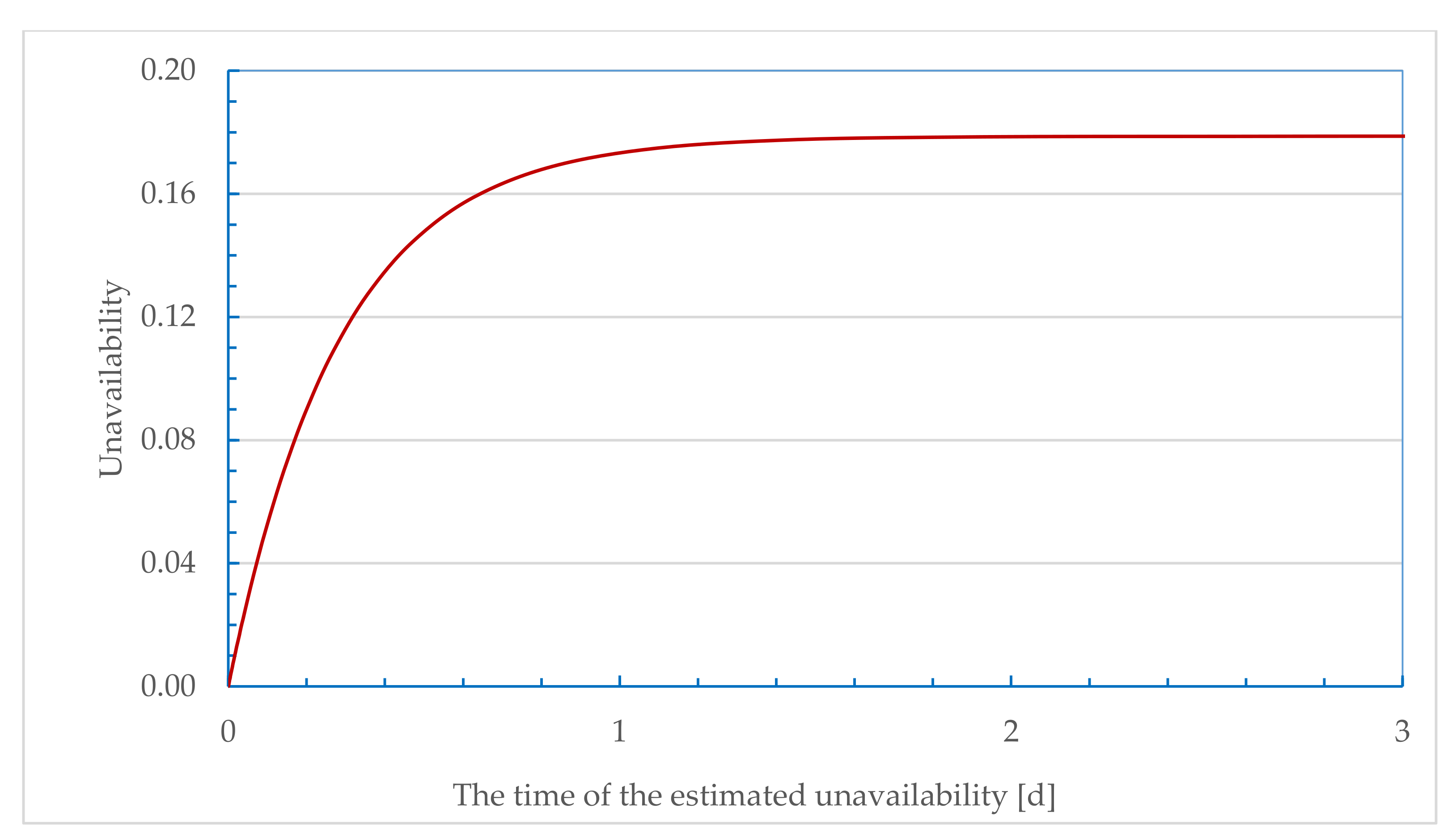
It is worth noting that the WSS attends $99.9\%$ of its asymptotic unavailability $u_{\infty }$ within $1.5$ days. So, we can state that the WSS attends its asymptotic time condition after $t=1.5$ days. The evolution with the time of the estimated unavailability $u\left(t\right)$ of the WSS is traced in days, Figure 9.

In addition, it is worth noting that the estimated rates are given in “per month”. Subsequently, the failure rate value of $18.8m^{-1}$ corresponds to $1.6d$ Mean Time Before Failure (MTBF), Equation (15), while the recovery rate value of $86.4m^{-1}$ corresponds to $0.347d$ Mean Time Before Recovery (MTBR), in “day” units.

4.2. The Reliability Model

Using the same classical model as in Appendix B, one can determine the meantime before failure as:

$$\widehat{\mathrm{MTBF}}=\frac{1}{{\lambda }_{WSS}}=\frac{1}{18.8}=0.0532t_m=1.6d,$$

(9)

Equation (9) is expected according to the survival analysis in system reliability theory as ${\lambda }_{WSS}$ is time-constant parameter. This is an overall meantime, considering all failure modes over all pipe-types and materials and everywhere in the network. It does not tell if the failure is significant or not, if it is on a main-pipe or a small connection, or if it is in winter or summer.

Still, it is a significant indicator as it tells us that a failure signal will be monitored each 1.5 days on average and its significance should be controlled to take the right action.

Another similar indicator is the number of failure signals $n$ expected per time interval $T$, which is the solution of:

$$P_n\left(T\right)=\underset{0}{\overset{T}{{\displaystyle \int }}}{P}_{n-1}\left(\tau \right)·\lambda d\tau ·Exp\left(-{\lambda }_{WSS}\left(T-\tau \right)\right),$$

(10)

where:

$P_n\left(T\right)$: is the probability of having $n$ failure signals, all failure types included, within an interval $T$.

$P_0\left(T\right)$: is the probability to have a zero-failure within the interval $T$ and is equal to

$$P_0\left(T\right)=Exp\left(-{\lambda }_{WSS}T\right),$$

(11)

The solution of the previous Equation (10) is:

$$P_n\left(T\right)=\frac{{\left({\lambda }_{WSS}T\right)}^n}{n!}Exp\left(-{\lambda }_{WSS}T\right),$$

(12)

The estimated distribution $P_n\left(T\right)$ of having $n$ failure-occurrences with the interval $T$ is traced in Figure 10.

The distribution $P_n\left(T\right)$ of having $n$ failure-occurrences with the interval $T$ allows us to determine two interesting measurables that are easily monitored and useful in assessing the performance of the WSS and the water supply system.

The first of these measurables is the expectation number $\widehat{n}$ of failure-occurrences within an interval $T$, such as:

$$\widehat{n}\left(T\right)=E\left(n\right)={\displaystyle \sum }_{n=1}^{\infty }n·P_n\left(T\right),$$

(13)

The expectation value $\widehat{n}$ is then determined as such:

$$\widehat{n}\left(T\right)={\displaystyle \sum }_{n=1}^{\infty }\left[n·\frac{{\left({\lambda }_{WSS}T\right)}^n}{n!}Exp\left(-{\lambda }_{WSS}T\right)\right]=\left({\lambda }_{WSS}T\right)·Exp\left(-{\lambda }_{WSS}T\right)·{\displaystyle \sum }_{n=1}^{\infty }\left[\frac{{\left({\lambda }_{WSS}T\right)}^{n-1}}{\left(n-1\right)!}\right],$$

(14)

Considering that:

$${\displaystyle \sum }_{n=1}^{\infty }\left[\frac{{\left({\lambda }_{WSS}T\right)}^{n-1}}{\left(n-1\right)!}\right]=Exp\left({\lambda }_{WSS}T\right),$$

(15)

Then expectation value $\widehat{n}$ is determined by:

$$\widehat{n}\left(T\right)={\lambda }_{WSS}T=\frac{T}{\widehat{\mathrm{MTBF}}},$$

(16)

The 2nd measurable is the most probable interval $T_{MP}$ within which $n$ failure-occurrence may be observed. This most probable interval occurs when:

$$\frac{d}{dT}{P}_n\left(T\right)=0,$$

(17)

We get than:

$$\left(1-\frac{{\lambda }_{WSS}T}{n}\right)·\frac{{\left({\lambda }_{WSS}T\right)}^{n-1}}{\left(n-1\right)!}·Exp\left(-{\lambda }_{WSS}T\right)=0,$$

(18)

Amongst the three possible solutions, the interval $T_{MP}$ that corresponds to the highest probability to observe $n$ failure-occurrences, $P_n\left(T_{MP}\right)$, is then:

$$T_{MP}=\frac{n}{{\lambda }_{WSS}}=n·\widehat{\mathrm{MTBF}},$$

(19)

Substituting $T_{MP}$ in Equation (17) results in the probability value $P_n\left(T_{MP}\right)$ for the time-interval $T_{MP}$, as following:

$$P_n\left(T_{MP}\right)=\frac{{\left(n\right)}^n}{n!}{e}^{-n},$$

(20)

The most probable intervals to observe $n=1,2,3,4$ failure-occurrences and their corresponding occurrence probabilities are given in

Table 3. The most probable intervals to observe $n$ failure-occurrences in the WSS.

Metric		$\mathit{n}=1$	$\mathit{n}=2$	$\mathit{n}=3$	$\mathit{n}=4$
${\mathrm{P}}_{\mathrm{n}}\left(\mathrm{T}\right)$	$\frac{{\left(\frac{\mathrm{T}}{1.6}\right)}^{\mathrm{n}}}{\mathrm{n}!}{\mathrm{e}}^{-\frac{\mathrm{T}}{1.6}}$	$\left(\frac{\mathrm{T}}{1.6}\right){\mathrm{e}}^{-\frac{\mathrm{T}}{1.6}}$	$\frac{{\left(\frac{\mathrm{T}}{1.6}\right)}^2}{2}{\mathrm{e}}^{-\frac{\mathrm{T}}{1.6}}$	$\frac{{\left(\frac{\mathrm{T}}{1.6}\right)}^3}{6}{\mathrm{e}}^{-\frac{\mathrm{T}}{1.6}}$	$\frac{{\left(\frac{\mathrm{T}}{1.6}\right)}^4}{24}{\mathrm{e}}^{-\frac{\mathrm{T}}{1.6}}$
${\mathrm{T}}_{\mathrm{MP}}\left(\mathrm{day}\right)$	$1.6\mathrm{n}$	$1\times 1.6$	$2\times 1.6$	$3\times 1.6$	$4\times 1.6$
${\mathrm{P}}_{\mathrm{n}}\left({\mathrm{T}}_{\mathrm{MP}}\right)$	$\frac{{\left(\mathrm{n}\right)}^{\mathrm{n}}}{\mathrm{n}!}{\mathrm{e}}^{-\mathrm{n}}$	$0.368$	$0.271$	0.224	0.195

.

To synthesise the learnings from Table 2, we underline that:

• One should expect to monitor $n$ failure-signals, each $1.6n$ days. The monitored signals do not indicate neither the mode nor the criticality of the failure in terms of water supply unavailability.
• The highest probability of monitoring, $n$ failure-signals within intervals equal to $1.6n$ days is equal to $\frac{{\left(n\right)}^n}{n!}{e}^{-n}$.

4.3. Measurable Indicators

The global model presented in the paper allows us to propose four measurable indicators to assess the WSS and the water supply service performance.

The 1st indicator is the expected asymptotic unavailability (Equation (5)), the second is the meantime before failure (Equation (9)), the third is the expected number of failures n within an interval T (Equation (16)), and the fourth is the expected interval $T_{MP}$ to observe n failures (Equation (19)). These four indicators can directly be estimated by the statistical analysis of the operational experience feedback data.

We should underline that the values estimated by the mathematical model will be called “expected values” while the term “estimated values” will be used for the values that are resulted from the statistical analyses of the operational data.

5. Predictivity and Control Indicators

In the preceding section, we have illustrated how the predictive models may help in developing indicators that are useful in controlling the WSS and the water supply services performance. The predictive quality of a mathematical model is conditioned by the founded concept of the model and the statistical quality of the basic data issued from the operational experience feedback. The predictive model proposed in the paper is based on:

• A binary functional concept that conceives the whole network as one single point (node) where only failure and recovery occur independently.
• Real operational experience feedback data covering 18 years of failure observations and 10 years of recovery data. Failure and recovery data are structured in different manners.

Even though both failure-recovery data have in many aspects a fair statistical quality, the resultant predictive indicators are still significant even if it is attached with some statistical uncertainties.

In Section 4, we presented four indicators: the asymptotic unavailability $u_{\infty }$, the meantime before a failure is monitored $\widehat{\mathrm{MTBF}}$, the expected number of failures $\hat{\mathrm{n}}\left(T\right)$ within an interval T, and the most probable interval $T_{MP}$ to observe $n$ failure-occurrences. These four indicators are interested because they are field direct measurables. They can be of great interest as the modernisation of the WSS will imply the use of the ICT for in-line monitoring and control activities.

These global indicators do not distinguish between failures severity, type, or location. However, they are very indicative regarding the qualification of the modernisation actions and the shared efforts between equipment technology ($\lambda$) and maintenance ($\mu$) logistic organisation.

The comparison between the operational estimated and the model expected values will allow us to validate and to better adjust the models. Subsequently, these predictive models present increasingly valuable support to the decision making in managing the modernization and the expansion the WSS and the water supply service performance.

As our models have been conceived to predict the indicators mentioned above based on the operational database, the validation of the model will be carried on after updating the operational databases including failure-recovery post-modernisation data.

For the time being, the conclusion of the assessment is still a predictive indicator.

6. Conclusions

Within the frame of the modernisation of a regional water supply system (WSS) in Poland, some R&D activities were conducted to develop predictive models to support decision making in managing the modernisation and the urban extension of the WSS. The modelling activities should be based on and validated by the operational experience feedback.

The operational experience feedback is generally available in the form of failure and recovery databases. The paper presents a case study to assess the failure and the recovery characteristic parameters of a given regional WSS in Poland. The assessment is carried out in two phases: the statistical analysis of the available operational data and the development of a predictive global modelling capability. The concerned databases are failure and recovery databases. In the failure database, one counts number of failures while one measures intervals of time-to-recover in the recovery database. Both measurables are random but different in nature.

Regarding the scope of the paper, the final outcomes we looked for are an “overall failure rate” and an “overall recovery rate” to globally characterise the WSS. These characteristic parameters are necessary to develop global predictive models of availability and reliability, to assess the quality of the water supply service and to support the decision making regarding the modernisation of the WSS.

Regarding the recovery database we have, it contains time intervals in two classes: physical component-repair times and associated organisational times, covering 10 years. The analyses considered the component-repair time ($T_c$) and the organisation-repair time ($T_o$) within the intention to estimate the WSS overall recovery-time, ($T_r$). The variability per year in the component-repair meantime $T_c$ is much more significant than in the organisational-repair meantime $T_o$, including the seasonality effect. However, the major contribution in the overall recovery-time is so far from the organisational repair time. Accordingly, one can then state that the characteristic WSS recovery repair rate ${\mu }_{WSS}$ is equal to ~ $\approx 2.9\times d^{-1}$.

Once the overall characteristic parameters (${\lambda }_{WSS},{\mu }_{WSS}$) are determined, one can then propose a classical model to predict unavailability and reliability based on the well-known system reliability theory and survival analysis. It is a binary point-like model as it considers the whole network as one node either available or unavailable. The estimated overall failure rate is mixing all failure modes, mechanisms, criticality, locality, and pipe functionalities. It overestimates the failures’ occurrence. Accordingly, the model is conservative as it overestimates the unavailability and underestimates the reliability.

The predictive model allows us to propose four indicators: the asymptotic unavailability $u_{\infty }$, the meantime before a failure is monitored ($\widehat{\mathrm{MTBF}}$), the expected number of failures $\hat{\mathrm{n}}\left(T\right)$ within an interval $T$, and the most probable interval $T_{MP}$ to observe $n$ failure-occurrences. These four indicators are interested because they are field direct measures. So, they are proposed to assess the effectiveness of the decisions and actions taken within the modernisation and the extension of the regional WSS.

In addition, they can be of great interest as the modernisation of the WSS will imply the use of the ICT for in-line monitoring and control activities.

The robustness of the predictive model and its control indicators will be assessed once the databases are updated by the integration of the post-modernisation failure-recovery data.

The proposed assessment, through the implementation of the failure and recovery analysis and scaled models based on the proposed global model, can be very helpful in developing the water safety plans as recommended by WHO [40] and the assessment of water leakage levels according to the revised Drinking Water Directive [41].