
The Estimation Life Cycle of Lithium-Ion Battery Based on Deep Learning Network and Genetic Algorithm


Abstract
:1. Introduction
2. Related Works
2.1. MLP (Multilayer Perceptron)
2.2. RNN (Recurrent Neural Network)
2.3. LSTM (Long Short-Term Memory)
2.4. GRU (Gated Recurrent Unit)
| Recurrent Neural Network Equation |
| The output of RNN: σ( ) is activation function. is the hidden layer activations in time t. is the input vector. is the weight of input vector. is the weight of hidden layer activations. is the bias. |
| Long Short Term Memory Equation |
| Forgotten gate: σ( ) is activation function. is the current forgotten gate. is the current input vector. is the current weight of input vector. is the weight of the hidden vector. is the weight of hidden vector in time t − 1. is the bias. Input gate: it = σ(Wxi × Xt + Whi × ht − 1 + bi) it is the external input gate. Output gate: Ot = σ(Wxo × Xt + Who × ht − 1 + bo) Ot is the output gate. is the output. |
| Gated Recurrent Unit Equation |
| Update gate: Zt is the update gate. Reset gate: Rt is the reset gate. |
3. Our Proposed Battery Model and Prediction Method
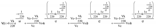
3.1. Battery Characteristics
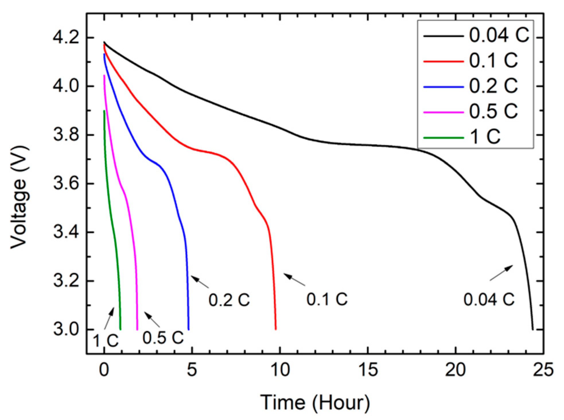
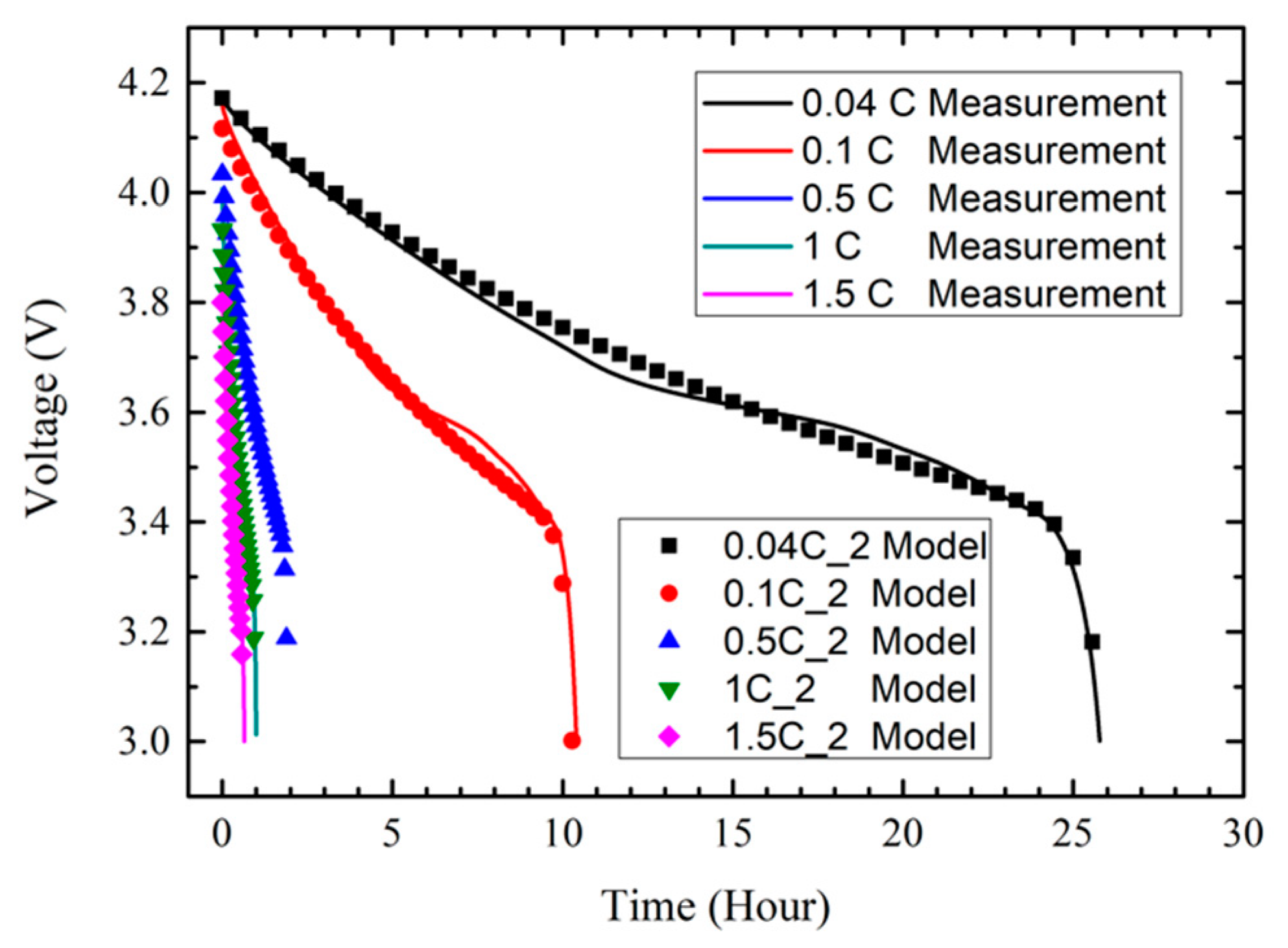
3.2. Lithium-Ion Battery Charge and Discharge
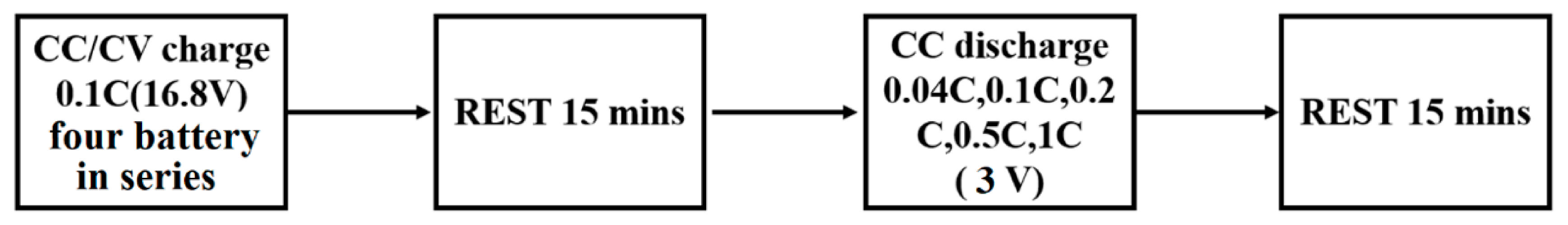
3.3. Lithium-Ion Battery Activation
3.4. Lithium-Ion Battery Charging and Discharging
3.5. Multilayer Perceptron
3.6. Recurrent Neural Network, Long Short Term Memory, and Gated Recurrent Unit
- In addition to the predicted output, a memory branch is added and updated over time. The current memory is represented by the “forget gate”, and “input gate” is used to determine whether to update the memory.
- Forget Gate: If the current sentence is a new topic or the opposite of the previous sentence, the previous sentence will be filtered out by this gate. Otherwise, it may continue to be retained in memory. This gate is usually a Sigmoid function.
- Input Gate: This determines whether the current input and the newly generated memory cell are added to the long term memory. This gate is also a Sigmoid function, which means that it needs to be added or not.
- Output Gate: This determines whether the current state is added to the output. This gate is also a Sigmoid function, indicating whether to add it or not.
- Finally, for whether the long-term memory is added to the output, the tanh function is usually used. The value of the output gate will fall between [−1, 1], and the −1 means removing the long-term memory.
3.7. Genetic Algorithm
4. Experiment Result
4.1. Manual Extraction Parameters
4.2. MLP Result
4.3. RNN Result
4.4. LSTM Result
4.5. GRU Result
4.6. GA Results
4.6.1. L Brand 18650
4.6.2. P Brand 18650
4.6.3. S Brand 18650
5. Discussion
6. Conclusions
Author Contributions
Funding
Conflicts of Interest
References
- Ahuja, D.; Tatsutani, M. Sustainable energy for developing countries. Surv. Perspect. Integr. Environ. Soc. 2009, 2, 1. [Google Scholar]
- Pereira, J.C. Environmental issues and international relations, a new global (dis)order-the role of International Relations in promoting a concerted international system. Rev. Bras. Política Int. 2015, 58, 191–209. [Google Scholar] [CrossRef] [Green Version]
- Bryntesen, S.; Strømman, A.; Tolstorebrov, I.; Shearing, P.; Lamb, J.; Burheim, O.S. Opportunities for the State-of-the-Art Production of LIB Electrodes—A Review. Energies 2021, 14, 1406. [Google Scholar] [CrossRef]
- Piller, S.; Perrin, M.; Jossen, A. Methods for state-of-charge determination and their applications. J. Power Sources 2001, 96, 113–120. [Google Scholar] [CrossRef]
- Shen, Y.C. The Characteristics of Battery Discharge and Automodeling. Master Thesis, National Taiwan Ocean University, Keelung, Taiwan, 2013. [Google Scholar]
- Lee, S.J.; Kim, J.H.; Lee, J.M.; Cho, B.H. The State and Parameter Estimation of an Li-Ion Battery Using a New OCV-SOC Concept. In Proceedings of the Power Electronics Specialists Conference, Orlando, FL, USA, 17–21 June 2007; pp. 2799–2803. [Google Scholar]
- Ehret, C.; Piller, S.; Schroer, W.; Jossen, A. State-of-charge determination for lead-acid batteries in PV-applications. In Proceedings of the 16th European Photovoltaic Solar Energy Conference, Glasgow, UK, 1–5 May 2000. [Google Scholar]
- Huet, F. A review of impedance measurements for determination of the state-of-charge or state-of-health of secondary batteries. J. Power Sources 1998, 70, 59–69. [Google Scholar] [CrossRef]
- Yu, Z.; Huai, R.; Xiao, L. State-of-Charge Estimation for Lithium-Ion Batteries Using a Kalman Filter Based on Local Linearization. Energies 2015, 8, 7854–7873. [Google Scholar] [CrossRef] [Green Version]
- Chan, C.; Lo, E.; Weixiang, S. The available capacity computation model based on artificial neural network for lead–acid batteries in electric vehicles. J. Power Sources 2000, 87, 201–204. [Google Scholar] [CrossRef]
- Hsieh, Y.; Tan, S.; Gu, S.; Jeng, Y. Prediction of Battery Discharge States Based on the Recurrent Neural Network. J. Internet Technol. 2020, 21, 113–120. [Google Scholar]
- Hsieh, Y.-Z.; Lin, S.-S.; Luo, Y.-C.; Jeng, Y.-L.; Tan, S.-W.; Chen, C.-R.; Chiang, P.-Y.; Hsieh, Y.-Z.; Lin, S.-S.; Luo, Y.-C.; et al. ARCS-Assisted Teaching Robots Based on Anticipatory Computing and Emotional Big Data for Improving Sustainable Learning Efficiency and Motivation. Sustainability 2020, 12, 5605. [Google Scholar] [CrossRef]
- Shahrivar, E.M.; Sundaram, S. The Strategic Formation of Multi-Layer Networks. IEEE Trans. Netw. Sci. Eng. 2015, 2, 164–178. [Google Scholar] [CrossRef] [Green Version]
- Vilovic, I.; Burum, N. A comparison of MLP and RBF neural networks architectures for electromagnetic field prediction in indoor environments. In Proceedings of the 5th European Conference on Antennas and Propagation (EUCAP), Rome, Italy, 11–15 April 2011; pp. 1719–1723. [Google Scholar]
- Xiang, C.; Ding, S.Q.; Lee, T.H. Architecture analysis of MLP by geometrical interpretation. In Proceedings of the 2004 International Conference on Communications, Circuits and Systems (IEEE Cat. No.04EX914), Chengdu, China, 27–29 June 2004; Volume 2, pp. 1042–1046. [Google Scholar] [CrossRef]
- Xiang, C.; Ding, S.Q.; Lee, T.H. Geometrical Interpretation and Architecture Selection of MLP. IEEE Trans. Neural Netw. 2005, 16, 84–96. [Google Scholar] [CrossRef] [PubMed]
- Rumelhart, D.E.; Hinton, G.E.; Williams, R.J. Learning representations by back-propagating errors. Nature 1986, 323, 533–536. [Google Scholar] [CrossRef]
- Uçkun, F.A.; Özer, H.; Nurbaş, E.; Onat, E. Direction Finding Using Convolutional Neural Networks and Convolutional Recurrent Neural Networks. In Proceedings of the 2020 28th Signal Processing and Communications Applications Conference (SIU), Gaziantep, Turkey, 5–7 October 2020; pp. 1–4. [Google Scholar] [CrossRef]
- Boden, M.; Hawkins, J. Improved Access to Sequential Motifs: A Note on the Architectural Bias of Recurrent Networks. IEEE Trans. Neural Netw. 2005, 16, 491–494. [Google Scholar] [CrossRef] [PubMed]
- Sepp, H.; Jürgen, S. Long Short-Term Memory. Neural Comput. 1997, 9, 1735–1780. [Google Scholar]
- Heck, J.C.; Salem, F.M. Simplified minimal gated unit variations for recurrent neural networks. In Proceedings of the 2017 IEEE 60th International Midwest Symposium on Circuits and Systems (MWSCAS), Boston, MA, USA, 6–9 August 2017; pp. 1593–1596. [Google Scholar] [CrossRef] [Green Version]
- Kumar, B.P.; Hariharan, K. Multivariate Time Series Traffic Forecast with Long Short Term Memory based Deep Learning Model. In Proceedings of the 2020 International Conference on Power, Instrumentation, Control and Computing (PICC), Thrissur, India, 17–19 December 2020; pp. 1–5. [Google Scholar] [CrossRef]
- Sheikhfaal, S.; Demara, R.F. Short-Term Long-Term Compute-in-Memory Architecture: A Hybrid Spin/CMOS Approach Supporting Intrinsic Consolidation. IEEE J. Explor. Solid-State Comput. Devices Circuits 2020, 6, 62–70. [Google Scholar] [CrossRef]
- Schmidhuber, J.; Gers, F.; Eck, D. Learning Nonregular Languages: A Comparison of Simple Recurrent Networks and LSTM. Neural Comput. 2002, 14, 2039–2041. [Google Scholar] [CrossRef] [PubMed]
- Liu, B.; Meng, P. Hybrid Algorithm Combining Ant Colony Algorithm with Genetic Algorithm for Continuous Domain. In Proceedings of the 2008 The 9th International Conference for Young Computer Scientists, Hunan, China, 18–21 November 2008; pp. 1819–1824. [Google Scholar] [CrossRef]
- Apostolov, P.S.; Stefanov, A.K.; Bagasheva, M.S. Efficient FIR Filter Synthesis Using Sigmoidal Function. In Proceedings of the 2019 X National Conference with International Participation (ELECTRONICA), Sofia, Bulgaria, 16–17 May 2019; pp. 1–4. [Google Scholar] [CrossRef]
- Komatsuzaki, Y.; Otsuka, H.; Yamanaka, K.; Hamamatsu, Y.; Shirae, K.; Fukumoto, H. A low distortion Doherty amplifier by using tanh function gate bias control. In Proceedings of the 2014 Asia-Pacific Microwave Conference, Sendai, Japan, 4–7 November 2014; pp. 110–112. [Google Scholar]
- Junyoung, C.; Caglar, G.; KyungHyun, C.; Yoshua, B. Empirical Evaluation of Gated Recurrent Neural Networks on Sequence Modeling. arXiv 2014, arXiv:1412.3555. [Google Scholar]
- Turan, A.; Kayıkçıoğlu, T. Neuronal motifs of long term and short term memory functions. In Proceedings of the 2014 22nd Signal Processing and Communications Applications Conference (SIU), Trabzon, Turkey, 23–25 April 2014; pp. 1255–1258. [Google Scholar] [CrossRef]
- Mirza, A.H. Online additive updates with FFT-IFFT operator on the GRU neural networks. In Proceedings of the 2018 26th Signal Processing and Communications Applications Conference (SIU), Izmir, Turkey, 2–5 May 2018; pp. 1–4. [Google Scholar] [CrossRef] [Green Version]
- Mirza, A.H. Variants of combinations of additive and multiplicative updates for GRU neural networks. In Proceedings of the 2018 26th Signal Processing and Communications Applications Conference (SIU), Izmir, Turkey, 2–5 May 2018; pp. 1–4. [Google Scholar] [CrossRef]
- Yang, S.; Yu, X.; Zhou, Y. LSTM and GRU Neural Network Performance Comparison Study: Taking Yelp Review Dataset as an Example. In Proceedings of the 2020 International Workshop on Electronic Communication and Artificial Intelligence (IWECAI), Qingdao, China, 12–14 June 2020; pp. 98–101. [Google Scholar] [CrossRef]
- Pavithra, M.; Saruladha, K.; Sathyabama, K. GRU Based Deep Learning Model for Prognosis Prediction of Disease Progression. In Proceedings of the 2019 3rd International Conference on Computing Methodologies and Communication (ICCMC), Erode, India, 27–29 March 2019; pp. 840–844. [Google Scholar] [CrossRef]
- Yichen, L.; Bo, L.; Chenqian, Z.; Teng, M. Intelligent Frequency Assignment Algorithm Based on Hybrid Genetic Algorithm. In Proceedings of the 2020 International Conference on Computer Vision, Image and Deep Learning (CVIDL), Nanchang, China, 15–17 May 2020; pp. 461–467. [Google Scholar] [CrossRef]
- Jiang, J.; Butler, D. A genetic algorithm design for vector quantization. In Proceedings of the First International Conference on Genetic Algorithms in Engineering Systems: Innovations and Applications, Sheffield, UK, 12–14 September 1995; pp. 331–336. [Google Scholar] [CrossRef]
- Wang, J.; Hong, W.; Li, X. The Influence of Genetic Initial Algorithm on the Highest Likelihood in Gaussian Mixture Model. In Proceedings of the 2006 6th World Congress on Intelligent Control and Automation, Dalian, China, 21–23 June 2006; pp. 3580–3583. [Google Scholar] [CrossRef]
- Chen, M.; Yao, Z. Classification Techniques of Neural Networks Using Improved Genetic Algorithms. In Proceedings of the 2008 Second International Conference on Genetic and Evolutionary Computing, Jinzhou, China, 25–26 September 2008; pp. 115–119. [Google Scholar] [CrossRef]
- Ananda, S.; Lakshminarasamma, N.; Radhakrishna, V.; Srinivasan, M.S.; Satyanarayana, P.; Sankaran, M. Generic Lithium ion battery model for energy balance estimation in spacecraft. In Proceedings of the 2018 IEEE International Conference on Power Electronics, Drives and Energy Systems (PEDES), Chennai, India, 18–21 December 2018; pp. 1–5. [Google Scholar] [CrossRef]


| L Brand | P Brand | S Brand | |
|---|---|---|---|
| Average voltage | 3.7 V | 3.7 V | 3.7 V |
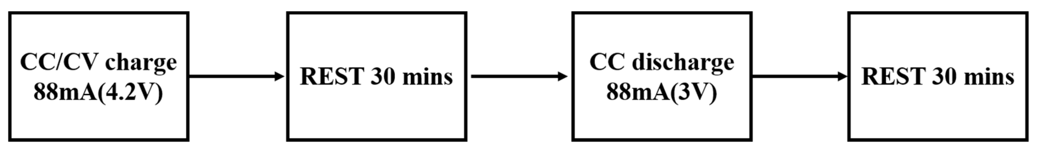
| Charging cut-off voltage | 4.2 V | 4.2 V | 4.2 V |
| Discharge cut-off voltage | 3.0 V | 3.0 V | 3.0 V |
| Nominal capacity | 2200 mAh | 2200 mAh | 2200 mAh |
| Maximum discharge rate | 1.5 C | 1.5 C | 1.5 C |
| Cycle life | ≥300 | ≥300 | ≥300 |
| Charging working temperature | 10 °C~45 °C | 10 °C~45 °C | 10 °C~45 °C |
| Discharge working temperature | −10 °C~60 °C | −10 °C~60 °C | ±10 °C~60 °C |
| L Brand 18650 | Score | P Brand 18650 | Score | S Brand 18650 | Score |
|---|---|---|---|---|---|
| C1E100LB10 | 2.3962 | C1E100LB10 | 1.9665 | C1E100LB10 | 1.416 |
| C2E100LB10 | 1.0355 | C2E100LB10 | 2.5641 | C2E100LB10 | 5.1457 |
| C3E100LB10 | 1.9235 | C3E100LB10 | 2.1702 | C3E100LB10 | 1.4973 |
| C4E100LB10 | 2.5563 | C4E100LB10 | 1.2151 | C4E100LB10 | 1.9197 |
| C5E100LB10 | 1.8657 | C5E100LB10 | 3.4141 | C5E100LB10 | 2.2744 |
| C6E100LB10 | 2.1928 | ||||
| C7E100LB10 | 1.8609 |
| L Brand 18650 | Score | P Brand 18650 | Score | S Brand 18650 | Score |
|---|---|---|---|---|---|
| C1E100LB10 | 22.7628 | C1E100LB10 | 26.1699 | C1E100LB10 | 10.2164 |
| C2E100LB10 | 12.8867 | C2E100LB10 | 15.3611 | C2E100LB10 | 11.8313 |
| C3E100LB10 | 19.2566 | C3E100LB10 | 7.8641 | C3E100LB10 | 16.3885 |
| C4E100LB10 | 16.4656 | C4E100LB10 | 13.1751 | C4E100LB10 | 47.0949 |
| C5E100LB10 | 14.4838 | C5E100LB10 | 27.3929 | C5E100LB10 | 23.4548 |
| C6E100LB10 | 12.1015 | ||||
| C7E100LB10 | 11.0649 |
| L Brand 18650 | Score | P Brand 18650 | Score | S Brand 18650 | Score |
|---|---|---|---|---|---|
| C1E100LB10 | 35.2445 | C1E100LB10 | 5.3272 | C1E100LB10 | 5.2539 |
| C2E100LB10 | 34.7757 | C2E100LB10 | 7.2181 | C2E100LB10 | 30.271 |
| C3E100LB10 | 16.183 | C3E100LB10 | 9.3963 | C3E100LB10 | 8.6395 |
| C4E100LB10 | 4.7719 | C4E100LB10 | 3.2441 | C4E100LB10 | 16.1969 |
| C5E100LB10 | 7.4273 | C5E100LB10 | 7.3323 | C5E100LB10 | 11.1258 |
| C6E100LB10 | 5.8578 | ||||
| C7E100LB10 | 3.7878 |
| L Brand 18650 | Score | P Brand 18650 | Score | S Brand 18650 | Score |
|---|---|---|---|---|---|
| C1E100LB10 | 11.7349 | C1E100LB10 | 13.9564 | C1E100LB10 | 7.9086 |
| C2E100LB10 | 22.561 | C2E100LB10 | 10.8346 | C2E100LB10 | 14.9015 |
| C3E100LB10 | 15.0054 | C3E100LB10 | 8.2631 | C3E100LB10 | 7.614 |
| C4E100LB10 | 5.245 | C4E100LB10 | 5.8903 | C4E100LB10 | 21.8592 |
| C5E100LB10 | 5.2089 | C5E100LB10 | 12.3002 | C5E100LB10 | 8.8804 |
| C6E100LB10 | 7.3077 | ||||
| C7E100LB10 | 5.1895 |
| Parameter | Range | True Value |
|---|---|---|
| I | 0.01~110 | 72.6875 |
| K | 1.4 × 10⁻¹³~1.4 × 10⁻¹⁹ | 1.3633 × 10⁻¹³ |
| Vk | 0~4000 | 3674 |
| Vc | 0~42,000 | 1292 |
| Vo1 | 0~3000 | 2404 |
| Vo2 | 0~35,000 | 10,603 |
| Vo3 | 0~4000 | 2555 |
| Vo4 | 0~70,000 | 30,444 |
| τ1 | 0~140,000 | 5339 |
| τ2 | 0~450,000,000 | 113,874,966 |
| τ3 | 0~187,000 | 55,007 |
| τ4 | 0~170,000 | 81,575 |
| τ5 | 0~10,000 | 604 |
| τ6 | 0~900,000,000 | 195,378,993 |
| Parameter | Range | True Value |
|---|---|---|
| I | 0.01~110 | 76.8125 |
| K | 1.4 × 10⁻¹³~1.4 × 10⁻¹⁹ | 9.1103 × 10⁻¹⁴ |
| Vk | 0~4000 | 2941 |
| Vc | 0~42,000 | 1087 |
| Vo1 | 0~3000 | 697 |
| Vo2 | 0~35,000 | 9232 |
| Vo3 | 0~4000 | 3554 |
| Vo4 | 0~70,000 | 8213 |
| Vo5 | 0~70,000 | 34247 |
| τ1 | 0~140,000 | 35186 |
| τ2 | 0~450,000,000 | 151,985,257 |
| τ3 | 0~187,000 | 7117 |
| τ4 | 0~170,000 | 87,017 |
| τ5 | 0~10,000 | 651 |
| τ6 | 0~900,000,000 | 155,079,888 |
| τ7 | 0~900,000,000 | 712,175,902 |
| Parameter | Range | True Value |
|---|---|---|
| I | 0.01~110 | 82.75 |
| K | 1.4 × 10⁻¹³~1.4 × 10⁻¹⁹ | 1.3061 × 10⁻¹³ |
| Vk | 0~4000 | 2965 |
| Vc | 0~42,000 | 1144 |
| Vo1 | 0~3000 | 2456 |
| Vo2 | 0~35,000 | 33,368 |
| Vo3 | 0~4000 | 2632 |
| Vo4 | 0~70,000 | 52,797 |
| Vo5 | 0~70,000 | 27,897 |
| τ1 | 0~140,000 | 139,951 |
| τ2 | 0~450,000,000 | 210,499,733 |
| τ3 | 0~187,000 | 2942 |
| τ4 | 0~170,000 | 47,774 |
| τ5 | 0~10,000 | 671 |
| τ6 | 0~900,000,000 | 818,734,152 |
| τ7 | 0~900,000,000 | 457,604,887 |
Publisher’s Note: MDPI stays neutral with regard to jurisdictional claims in published maps and institutional affiliations. |
© 2021 by the authors. Licensee MDPI, Basel, Switzerland. This article is an open access article distributed under the terms and conditions of the Creative Commons Attribution (CC BY) license (https://creativecommons.org/licenses/by/4.0/).
Share and Cite
Tan, S.-W.; Huang, S.-W.; Hsieh, Y.-Z.; Lin, S.-S. The Estimation Life Cycle of Lithium-Ion Battery Based on Deep Learning Network and Genetic Algorithm. Energies 2021, 14, 4423. https://doi.org/10.3390/en14154423
Tan S-W, Huang S-W, Hsieh Y-Z, Lin S-S. The Estimation Life Cycle of Lithium-Ion Battery Based on Deep Learning Network and Genetic Algorithm. Energies. 2021; 14(15):4423. https://doi.org/10.3390/en14154423
Chicago/Turabian StyleTan, Shih-Wei, Sheng-Wei Huang, Yi-Zeng Hsieh, and Shih-Syun Lin. 2021. "The Estimation Life Cycle of Lithium-Ion Battery Based on Deep Learning Network and Genetic Algorithm" Energies 14, no. 15: 4423. https://doi.org/10.3390/en14154423
APA StyleTan, S.-W., Huang, S.-W., Hsieh, Y.-Z., & Lin, S.-S. (2021). The Estimation Life Cycle of Lithium-Ion Battery Based on Deep Learning Network and Genetic Algorithm. Energies, 14(15), 4423. https://doi.org/10.3390/en14154423