1. Introduction
To control the movement of aircraft in accordance with the required trajectory, it is necessary to be able to change the magnitude and direction of the velocity vector in flight, as well as the orientation of the aircraft axes in space. Different thrust vector control (TVC) systems for solid propellant rocket motors (SRMs) based on various principles are classified in
Figure 1. Thrust vector control with the injection of the gas jet into a nozzle is relatively simple without the need for high-temperature sealing due to the structural decoupling of the SRM nozzle from the TVC system, reducing the thermal loading [
1,
2].
To create a control force in rocket engines, gas injection into the supersonic part of the nozzle is used [
3,
4]. The generated control force consists of two components, the thrust of the injection nozzle and the force applied to the walls of the main nozzle and arising from the redistribution of the pressure in the region of the interaction of the flows [
5]. The magnitude of the control force depends on the location of the injection hole, the injection angle and the pressure ratio of the injection nozzle. The shape and intensity of the disturbed zone are influenced by the flow rate and the parameters of the main flow, the flow rate and thermodynamic properties of the injected substance, as well as possible chemical reactions between the main flow and the injected substance [
6].
Many experimental, theoretical and numerical studies have been performed in the past few years to improve the current understanding of complex flows in the combustion chamber of an SRM. The accuracy and reliability of the computational results is affected by the choice of the turbulence model and the computational methods. The one-equation turbulence models allow obtaining a good agreement between the experimental and computational results of the mean flowfield at a low injection rate [
7]. However, one-equation turbulence models overpredict the intensity of the turbulence. To achieve a better agreement between the experimental and computational data at a high injection rate, two-equation turbulence models were applied in [
8] for a nozzleless SRM. These models provide more accurate results in terms of the intensity of the turbulence and the axis velocity distributions. In order to capture the viscous flow physics, the axisymmetric Navier–Stokes equations and the
k–
turbulence model equations were solved in [
9,
10] to resolve the flowfield near the mass-injecting propellant surface and wall regions. The large-eddy simulation of the effect of the high injection rate on the boundary layer development was investigated in [
8].
The methods of computational fluid dynamics (CFD) are extensively used in the solid design and optimization of TVC. A multidisciplinary design and optimization approach to optimize the nozzle, combustion chamber and solid fuel charge was developed in [
11] based on the use of analytical expressions (the mass of the charge was minimized). Multiparameter optimization based on the application of the thermodynamic approach to the calculation of the flow parameters was carried out in [
12]. To optimize the shape of the nozzle to provide the maximum thrust, the results of the simulation of flows of an inviscid and viscous compressible gas were applied in [
9,
10]. The flow in the nozzle and the stress–strain state of the nozzle walls (coupled modeling) associated with the occurrence of asymmetric loads were discussed in [
13].
The experimental data from [
14,
15] showed that the most effective, from the point of view of thrust vector control, is the location of the injection hole from the main nozzle outlet at a distance of about 20–30% of the length of its supersonic part. In overexpansion modes, the flow is separated from the walls. The cases when flow separation occurs behind the injection hole and in front of the injected jet are of particular interest. In some cases, it is possible to obtain a negative control force (reversed thrust). The influence of the angle of injection of a jet into a supersonic flow on the intensity and mixing rate of flows was considered in [
16].
The influence of the shape of the injector outlet section (round, square, diamond-shaped, triangular) on the vortex structure of the flow in the channel, the mixing mechanism and the stabilization of the combustion process was discussed in [
17,
18,
19,
20]. The shape of the outlet section of the injector has a relatively weak effect on the mixing efficiency in a wide range of pressure ratios, varying from 1.5% at low-pressure ratios in the injected and main flow to 5.4% at high-pressure ratios (injection of a hydrogen jet into the air flow). The width of the slotted nozzle varies from 0.1 to 0.5 mm, which at a fixed pressure ratio leads to a change in the length of the recirculation zone and the depth of penetration of the jet into the supersonic flow in a close to linear relationship [
21]. The optimization of the injection parameters carried out in [
20] (injection of a sonic jet from the surface of a flat plate into a supersonic flow with a Mach number of 3.5) included the choice of the pressure ratio in the injected jet and in the main flow, the position of the injection hole, the injection angle, the size of the injection hole and the molecular weight of the injected gas. In [
22], the calculations were carried out with the RNG (Re-Normalization Group)
k–
turbulence model. The jet was injected into the supersonic part of the nozzle through holes located at a distance of
,
, and
from the critical section of the main nozzle with a diameter of
.
The interaction of an oblique shock wave, formed as a result of the interaction of a supersonic flow in a channel with an inclined rib, with an injected jet was discussed in [
23]. The geometric model corresponded to that used in the experimental study [
15], and the calculations were carried out at low- (with the RNG
k–
model) and high- (with the SST model) pressure ratios [
21]. Calculations with the SST turbulence model were also carried out in [
24] at high-flow temperatures. Various turbulence models were compared with the measured data in [
25]. The injection of a stationary and pulsed jet from the surface of a flat plate into a supersonic flow was investigated in [
26,
27], and the injection of a jet into the supersonic part of the nozzle was studied in [
28]. A large-eddy simulation of transverse jet injection into a supersonic flow was performed in [
29]. The effects of different injection schemes on a transverse jet in a supersonic crossflow were discussed in [
30,
31,
32]. The implementation of the required value of the control force at the minimum flow rate of the injected gas was carried out when the injection hole was located at a distance of 0.3–0.4 of the length of the main nozzle from its outlet and the injection angle was 110–130
towards the nozzle axis towards the flow [
33,
34].
The combined CFD and multidesign optimization method with the data mining method, variance analysis method and extreme difference analysis was applied to solve various design problems in scramjet engines with multiple objective functions [
35,
36].
Although many experimental and computational studies have been performed, the information about the transverse injection flowfield has not been explored to quantify the thrust and improve the mixing process between the injected gas and the main nozzle flow. In this study, the interaction of a transverse jet with a supersonic flow in a nozzle is considered, and the problem of the multiparameter optimization of the operation of jet thrust vector controls is solved. The influence of the parameters of the problem, such as the pressure ratio of the injected jet, the angle of inclination of the injection nozzle to the axis of the main nozzle, the distance of the injection nozzle from the critical section of the main nozzle and the shape of the outlet section of the injection nozzle, on the coefficient of the amplification of the nozzle thrust is discussed. The developed approach allows finding the most effective combination of the product parameters. The relationships between the objective function of the independent variables are described by the Navier–Stokes equations and the equations of the turbulence model, while the relationships connecting the target and independent variables are nonlinear.
An unsteady complex three-dimensional flowfield was induced in the main nozzle when a secondary gas jet was injected. The resulting flowfield is characterized by the formation of a bow shock, a Mach disc, a boundary layer separation upstream of the injection port and its reattachment downstream of the injection port. A series of CFD simulations were conducted to demonstrate the thrust vectoring with gas injection system’s ability to control the orientation of the solid propellant engine. The motivation of the study came from the requirement of improving the current understanding and modeling capabilities of complex flows in TVC. The paper is organized as follows. The governing equations are presented in
Section 2. The details of the optimization procedure are presented in
Section 3. The geometric model of the thrust vector control system with gas injection and the details of mesh are discussed in
Section 4 and
Section 5. The numerical method used in the CFD calculations is presented in
Section 6. The results obtained are reported and analyzed in
Section 7. Conclusions are drawn in
Section 8.
2. Governing Equations
The in-house compressible CFD code was used to perform the numerical calculations. The working substance was air, which was treated as a perfect gas.
In Cartesian coordinates
, the unsteady three-dimensional viscous compressible flow is described by the equation:
Equation (
1) is supplemented with the equation-of-state of an ideal gas:
The vector of conservative variables
Q and the flux vectors
,
,
have the form:
Here, t is the time, is the density, , , and are the velocity components in the x, y, and z directions, p is the pressure, e is the total energy per unit mass, T is the temperature and is the ratio of the specific heat capacities.
Equation (
1) is suitable for the simulation of laminar and turbulent flows. It coincides with the unsteady Reynolds-averaged Navier–Stokes (RANS) equations. The components of the viscous stress tensor and the components of the heat flux are given by:
The effective viscosity,
, is found as the sum of the molecular viscosity,
, and the eddy viscosity,
. The effective thermal conductivity,
, is expressed in terms of the viscosity and the Prandtl number. The effective viscosity and thermal conductivities are found as follows:
where
is the specific heat capacity at constant pressure. The molecular and turbulent Prandtl numbers are
and
for air. Sutherland’s law is used to obtain the molecular viscosity as a function of temperature:
where
and
are the reference viscosity and temperature, and
is a constant determined experimentally, so that
kg/(m·s),
K, and
K for air. The turbulent eddy viscosity is obtained from the SST turbulence model.
The velocity profiles of the vortical inviscid incompressible flow in the channel with fluid injection are applied to a specified initial flowfield. This is a good and accurate representation of the real flowfield in the propellant channel (propellant burning is replaced with the fluid injection from the channel walls) [
5]. The flow near the head-end of the propellant channel is laminar, and a self-similar solution provides the distributions of the axial and radial velocities. For a uniform injection velocity from the channel walls,
, the velocity profiles are given as:
where
s is 0 for planar flow and
s is 1 for axisymmetric flow. In Equation (
2),
is the injection velocity on the propellant surface,
is the axial velocity,
is the radial velocity,
x and
y are the axial and radial coordinates and
h is the channel half-width or radius.
Compressibility has little affect on the flow quantities in the propellant channel where the flow velocities are subsonic. However, compressibility has a significant impact on the flow quantities in the nozzle where the flow velocity reaches supersonic values [
37]. To take into account the density variability in the CFD calculations, a semi-empirical correction to the source terms of turbulence model is applied. This correction assumes that the source terms are a function of the turbulent Mach number.
3. Optimization Procedure
The method used to construct the optimal solution is determined by the type of mathematical model. In most cases, the mathematical model of an object is represented as an objective function , where is the vector of the geometric parameters and flow quantities. It is maximized or minimized (optimization criterion). The range of permissible values is set, which is determined by a system of linear or nonlinear constraints. The complexity of the problem depends on the type of criterion and functions that determine the permissible optimization region.
In the process of designing complex systems, the problem of multi-objective optimization often arises, which is associated with the need to ensure the optimal design according to several optimization criteria. Usually, these criteria are contradictory, and the optimization of each of them leads to different values for the vector of varied parameters.
The optimization problem is solved in several steps:
The parametrization of the investigated model based on ideas about the ongoing physical phenomena. This step allows one to automatically generate a multiblock or unstructured mesh in the specified area;
The solution of a series of optimization problems for this model. The tasks are set based on the possible modes of operation of the system under study;
The systematization of the best obtained options for the formation of equations describing the optimal state of the system in the specified range of the boundary conditions.
The solutions of CFD problems significantly depend on the quality of the setting of the boundary conditions and the choice of the mesh and model parameters (for example, the turbulence model, the mesh resolution in the near-wall region). The extrapolation of the obtained conclusions beyond the solution of the problem requires taking into account additional physical effects. When setting the optimization problem, it is necessary to check various approaches and combinations of the control parameters and to determine the range of variation of each of the values and other factors that affect the speed and quality of the implementation of the optimization algorithm.
The use of modern computing systems to solve the Navier–Stokes equations allows an almost unlimited number of numerical experiments with various design solutions to be carried out, thereby replacing expensive field tests. The design of rocket engines is subject to many constraints and requirements, which tend to conflict with each other. The optimization problem is formulated as maximizing the specific thrust for some design parameters. The solution to the problem is a certain combination of the geometric parameters that provide the maximum values of specific thrust. For this, a sequential change in the geometric parameters of the model is carried out, and the objective function is recalculated.
The computational procedure associated with the optimization of injection controls is explained in
Figure 2. In the first stage, the optimizer generates a vector of variable parameters (angle and place of injection, shape of the cross-section of the injection nozzle, pressure ratio of the injected jet), and their values are written to a file. Based on these data, the geometry of the parametric model is automatically corrected in the Unigraphics NX (Siemens PLM Software, Plano, US) 3D solid modeling environment and saved. This is followed by launching the mesh generator Ansys ICEM CFD (Ansys UK Ltd, Abingdon, UK). Due to the fact that when the configuration of the computational domain is changed, its topology is preserved, it is possible to automatically generate the computational mesh using the prepared script file. The process of importing the mesh and setting the types of boundary conditions is also performed automatically using scripts. The mesh and boundary conditions are transferred to the computational module, which solves the CFD problem for a fixed set of parameters. The cycle is repeated with a modified vector of the input parameters of the problem to find their optimal values.
The optimization procedure involves automatic interaction among the optimizer, mesh generator and CFD code. The script file containing the parameterized geometric variables and the list of commands is read by the application, which generates the computational mesh, which is written to the file. The CFD code is then used to compute the flow on the mesh read from the file. All settings of the mathematical model and the list of required commands are in the script file. After receiving the converged solution, the calculations of the output variables are performed and they are written to the output data file. The system reads them and evaluates the data in accordance with the target optimization functions. Iterations are performed until a converged solution and a given level of the objective function are reached.
The function uses the conjugate gradient method to find the local extremum [
38]. Since the optimization criterion is given in the form of an implicit function, the partial derivatives at a given point are found using approximate formulas. Along with the definition of the gradient vector, the main issue is the choice of the step of movement along the gradient. The choice of the step size depends on the type of surface (a small step requires lengthy calculations, and a large step leads to the inaccurate determination of the position of the extremum).
4. Geometric Model
The geometric model of the propulsion system includes a cylindrical channel of a solid propellant with slotted holes and a submerged nozzle (
Figure 3a). The geometry of the solid propellant channel is designed to provide the required law of variation of the combustion rate and pressure in the combustion chamber.
The most interesting is the supersonic flow region where transverse jet injection takes place. The subsonic part of the nozzle and the previous section of the propellant channel are not included in the computational domain (it is supposed that flow disturbances are not transferred upstream). The calculations are carried out in the part of the domain shown in
Figure 3b. The discrepancy between the Mach numbers computed with full and shortened domains does not exceed 1%. This confirms the possibility of the use of domain decomposition [
25].
For the specification of boundary conditions in the inlet section, the flow is calculated in the full domain, including the propellant channel and the nozzle block (in the calculations,
). When the injection of the secondary jet is simulated, the inlet section of the domain is located at a sufficient distance from the injection nozzle. The mass flow rate (
kg/s), the total temperature (
K) and the radial profiles of the velocity and turbulence quantities computed from the axisymmetric calculations of the flow of combustion products in the propellant channel described by Equation (
2) are specified in the inlet section of the computational domain. The static pressure is set in the outlet section of the nozzle. In the case of a supersonic flow, the pressure in the outlet section of the nozzle is found by extrapolating the solution from the internal nodes, and in the case of a subsonic flow at the outlet, atmospheric pressure is used.
The total pressure (this parameter varies to obtain the required pressure ratio), the total temperature ( K) and turbulence quantities (the degree of turbulence is 0.1%, and the hydraulic diameter is 1.6 mm) are applied to the inlet section of the secondary nozzle. For the velocity on the nozzle surface, the no-slip and no-penetration boundary conditions are used. The walls of the nozzle are considered to be thermally insulated. The characteristics of turbulence on the wall are found using the method of wall functions.
5. Computational Mesh
To generate a block-structured mesh, the physical domain is divided into a number of nonoverlapping blocks, in each of which the mesh resolution is selected based on the gas dynamic features of the flow. The computations of the flow in a nozzle with a transverse injection of a jet are carried out on a mesh containing about 1.2 million cells (the mesh step size changes insignificantly when the configuration of the injection nozzle is changed). The mesh nodes are condensed near the throat of the nozzle and near the injection nozzle. Mesh nodes are also thickened near the nozzle walls to properly resolve the boundary layer. The range of variation of the variable parameters is shown in
Table 1, where
is the length of the supersonic part of the nozzle.
The computational meshes used for the numerical simulation of gas jet injection into the nozzle are shown in
Figure 4,
Figure 5,
Figure 6,
Figure 7,
Figure 8 and
Figure 9 for different angles of inclination of the injection nozzle to the axis of the main nozzle and for different distances of the injection nozzle from the throat of the nozzle. In this case,
is the relative distance from the critical section of the main nozzle to the outlet of the injection nozzle,
is the angle of inclination of the injection nozzle to the axis of the main nozzle,
and
are the length of the small and the major axes of the ellipse forming the outlet section of the injection nozzle and
and
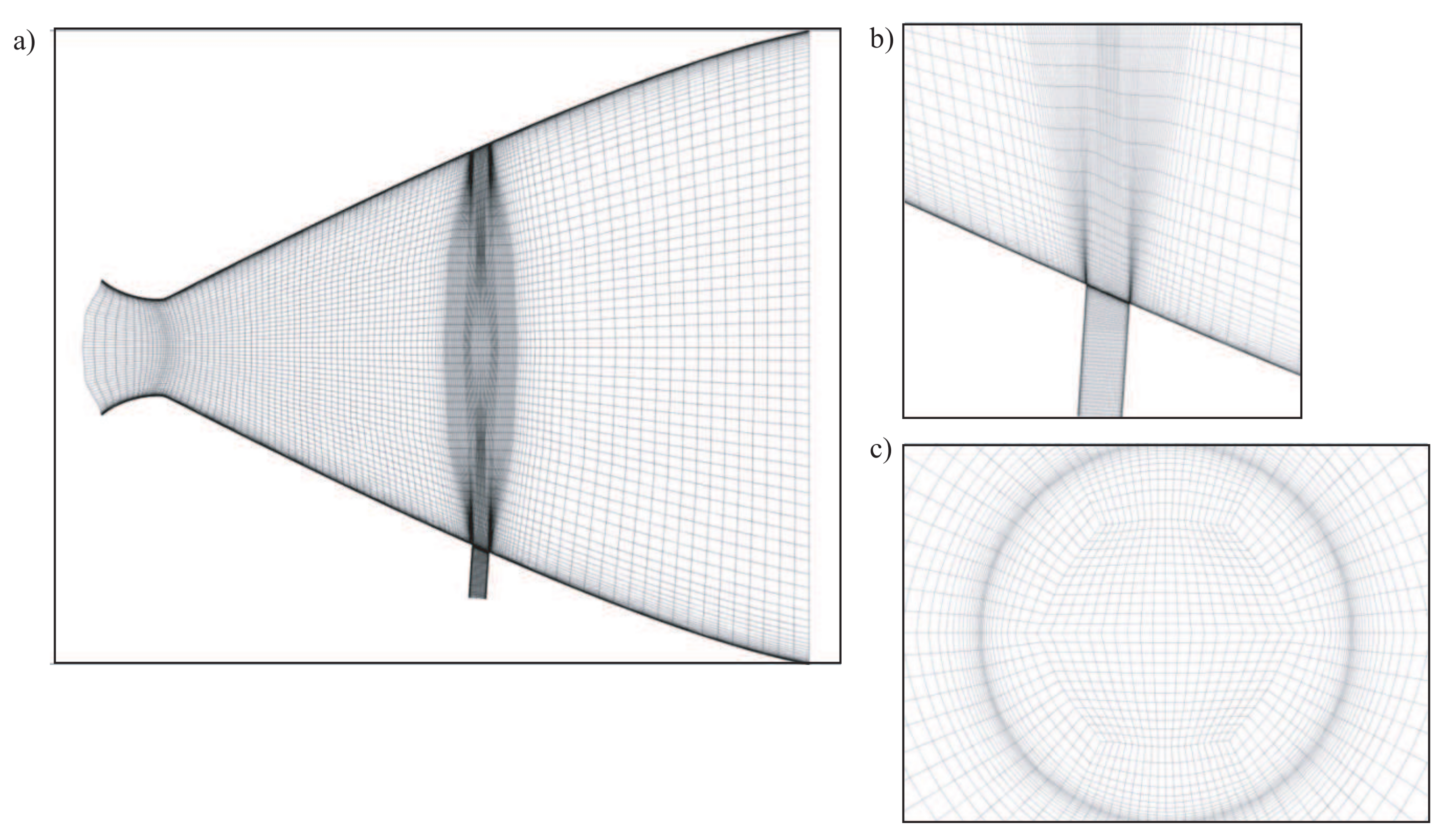
are the areas of the critical and outlet sections of the injection nozzle. Fragment a shows meshes in the entire computational domain, and Fragments b and c show the mesh corresponding to the injection nozzle and the place of its interface with the main nozzle and the mesh in the outlet section of the injection nozzle. The meshes are automatically generated from the parameterized geometric model. The quality criteria of the constructed meshes are the degree of cell skewness and the ratio of its sides (the difference between the mesh cell from a square or a cube), as well as the value of the dimensionless wall coordinate (
for the SST turbulence model).
The computational meshes shown in
Figure 4 and
Figure 5 differ in the place of the jet injection and the angle of inclination of the secondary nozzle to the axis of the main nozzle. The injection nozzle is a pipe with a circular cross-section in plan, installed at a certain angle to the nozzle axis.
The computational meshes shown in
Figure 6 and
Figure 7 differ in the shape of the injection nozzle. The jet is injected through a pipe with a circular or elliptical cross-sectional shape in plan, set at an angle to the nozzle axis.
The computational meshes shown in
Figure 8 and
Figure 9 correspond to nozzles with different area ratios. For injection, a pipe with an elliptical cross-section in plan or a converging–diverging nozzle with an elliptical outlet section is used.
The characteristics of the different meshes are shown in
Table 2 for various distances between the inlet section of the main and secondary nozzles, the angle of inclination of the secondary nozzle and the shapes of the secondary nozzle. The number of nodes and the quality of different meshes slightly depend on the geometrical configuration used in the CFD calculations. The maximum value of the
coordinates is observed near the separation region. The separation region increases if the angle of inclination of the injection nozzle increases.
7. Results and Discussion
The results were computed with the in-house CFD code for a wide range of input parameters characterizing the TVC system. The results of the optimization of TVC are also presented.
7.1. Flow in the Propellant Channel
The calculations of the flow in the propellant channel with a circular cross-section and containing slotted holes were carried out at a Reynolds number
. The results processed in the form of the Mach number level lines are shown in
Figure 10. The flow in the propellant channel was subsonic (
). At the nozzle outlet, the Mach number reached 3.8. The pressure in the propellant channel varied insignificantly, being practically uniform along the channel length (before entering the nozzle block). When flowing through the nozzle, the temperature decreased from 3600 K in the charge channel and in the prenozzle volume to 1772 K in the nozzle outlet section. Turbulence generation began at the section
, where
L is the channel length.
The flowfield in the combustion chamber and submerged nozzle of an SRM is complex. The flow velocity in the propellant channel increases from the head-end leading to nonuniform profiles of streamwise velocity. Then, flow undergoes a transition to turbulence in the midsection of the propellant channel and becomes fully turbulent further downstream. Finally, the flow velocity reaches supersonic conditions at the outlet of the nozzle. The velocity profiles and turbulence properties affect the convective heating loads and potential erosive burning of the propellant. The internal flowfield in the SRM was in qualitative and quantitative agreement with experimental, theoretical and computational studies in which the mean velocity and turbulent kinetic energy fields have been studied. The mean flowfield is represented by the vortical inviscid velocity profile described by Equation (
2) in the forward region of a cylindrical port rocket chamber. The simulations performed at various mass flow rates from the propellant surface showed that the laminar velocity profile persists in the mean flow, even if the flow is highly turbulent over the duct cross-section.
The shape of the sonic line at various pressure drops is shown in
Figure 11. The position of the sonic line on the jet axis is at a distance of about half of the nozzle radius from its outlet section. As the pressure drop increases, the sound line moves to the nozzle outlet. When a certain critical pressure drop is exceeded, the shape and position of the sonic line do not change (while the flow coefficient also remains practically constant).
7.2. Flow Regimes
Three different regimes of flow are observed in the propellant channel (
Figure 12). These regimes include the laminar regime (Region 1), the transitional regime (Region 2) and the turbulent regime (Region 3). It is interesting to note that viscous effects are important in the narrow region near the channel head-end (
). The flow is laminar if
. Then, the flow undergoes transitions to turbulence (
). Here, there is a difference in terms of turbulence generation in the channel with solid walls and the channel with fluid injection. In flow induced by fluid injection channel, turbulence generation is observed away from the walls (shaded region in the picture). The region with the maximum value of turbulent kinetic energy moves towards the wall and downstream direction (
) because fluid injection from the propellant surface does not allow flow disturbances to penetrate into the core region.
The profiles of axial velocity predicted with the developed model (solid lines) are flatter in the core region and steeper in the near-wall region than those computed in vortical flow (dashed lines). The distributions of the radial velocity computed with RANS and the model of vortical flow are in a good agreement. Compressibility effects play an important role in a long channel, leading to a more filled profile of axial velocity. The impact of the Reynolds number on the profiles of the axial and radial velocities in the flow induced by wall injection is small.
7.3. Distributions of Flow Quantities
In the presence of the injection of a jet into the nozzle, the CFD calculations were carried out for different angles of inclination of the injection nozzle to the axis of the nozzle, different distances of the injection nozzle with respect to the critical section of the nozzle and different shapes of the outlet section of the injection nozzle.
The pressure in front of the secondary jet increases, and a head shock is formed. An oblique shock wave extends upstream from the head shock. Behind the oblique shock, in addition to the separation region, there is a section of the supersonic zone. The subsequent deceleration of the flow is accompanied by the appearance of a closing shock wave, which is practically parallel to the jet axis. The detached bow shock and oblique and closing shock waves, intersecting at one point, form a complex
-shaped system of shock waves. The pressure along the forward boundary of the jet is maximum in the region lying behind the lower part of the closing shock [
41]. In the zone adjacent to the wall, in front of the jet, there are two vortices formed as a result of the primary and secondary separation of the flow from the wall. The directions of movement in them are opposite, since a part of the flow directly near the wall, passing the sections of the shock waves, turns downward towards the wall and penetrates into the zone of separated flow, then spreads out in opposite directions. In this case, the vortex located closer to the jet moves counterclockwise, and the vortex located at a greater distance from the jet moves clockwise.
The Mach number contours are shown in
Figure 13 for different angles of inclination of the injection nozzle to the axis of the main nozzle (injection was carried out opposite the main flow). An increase in the injection angle, with other parameters being the same, leads to an increase in the size of the front separation zone, as well as to a decrease in the depth of the penetration of the jet into the supersonic flow.
The pressure contours for various pressure ratios are shown in
Figure 14. As a result of the injection, there is a sharp increase in pressure in the separation region located in front of the injection nozzle, and a decrease in pressure in the separation region located behind the injection nozzle. Depending on the pressure ratio of the injected jet, the pressure distribution in the anterior separation region has one maximum or two maxima.
The shock wave structure is similar to those observed in [
25]. The main components of flowfield are shown in
Figure 15. These components include the upstream recirculation region (1), the bow shock (2), compression shocks (3), the curvilinear boundaries of the secondary jet (4), the Mach disc (5), the downstream recirculation region with vortices of various scales (6), the secondary jet (7) and the shock wave due to repeated compression (8). The boundary layer separation occurs at point S, and boundary layer reattachment occurs at point S.
The pressure distribution along the nozzle wall is shown in
Figure 16 for various pressure ratios. The solid line corresponds to the pressure distribution in the presence of injection and the dashed line to the pressure distribution in the absence of injection. The comparison of the solutions obtained without viscous effects and with viscous effects shows that taking viscous effects into account is important in the presence of boundary layer separation in overexpansion modes. The lateral control force is formed as a result of an increase in pressure on the nozzle surface in the separation zone between the beginning and end of the base of the
-shaped shock and behind it, as well as due to a decrease in pressure behind the injection nozzle.
Once the simulation has been performed, the length of the recirculation region is easily determined via the velocity vectors or the streamline plot. In the recirculation zone, the velocity vectors are in the opposite direction of the incident flow; however, at the end of this zone, the velocity vectors change their direction again towards the incident flow direction. The penetration depth of a secondary jet is defined as the distance between the nozzle wall and the location of the Mach disk, which if formed during the entrainment process and the interaction of the secondary jet and the supersonic nozzle flow [
42].
The length of the recirculation region and the depth of jet penetration into the main nozzle flow are presented in
Figure 17. These quantities are of interest for flow mixing of fuel and air in scramjet engines. Increasing the pressure ratio leads to an increase in the length of the recirculation region and the depth of jet penetration.
7.4. Optimization Results
The design of experiment methodology was employed to arrange the numerical cases. The design variables include the pressure ratio in the injected jet and the main nozzle flow, the position of the injection nozzle, the injection angle and the shape of the injection nozzle outlet. The axial thrust augmentation is defined as:
where
and
are the primary axial thrust with and without injection. The primary axis thrust is found as:
where
is the total outlet mass flow rate,
is the velocity along
x axis,
is the outlet pressure and
is the atmospheric pressure.
The thrust ratio is defined as the ratio of the side and axial forces,
. The side force is found from the relation
, where
is the interaction force (side force pressure component) and
is the jet reaction force (side force momentum component. The side force pressure component is calculated as the integral over the cross-sectional area from the pressure distribution on the nozzle wall. The side force momentum component is defined as:
where
is the secondary mass flow rate,
is the secondary gas velocity along the
y direction,
is the secondary outlet pressure,
is the atmospheric pressure at the secondary port before injection and
is the wall angle at the point of injection.
The control force consists of two components. The first component is the secondary jet thrust, and the second one is the force due to the pressure redistribution induced by the interaction of the secondary jet with the main supersonic flow. The injection efficiency is estimated in relation to the thrust of a conventional engine having the same flow rate as the secondary gas flow rate and the same specific thrust as the main nozzle. The ratio of the lateral injection force to the thrust of the corresponding conventional engine is a gain that depends on the relative flow rate of the injected gas and the injection conditions. The influence of the pressure ratio on the thrust amplification factor is shown in
Figure 18. It is interesting to note the presence of a negative control effort at low degrees of off-design (at
). The thrust characteristics are shown in
Figure 19 depending on the angle and place of injection of the jet into the supersonic part of the nozzle.
Upstream injection increases the axial thrust augmentation for the given mass flow rate. This is explained by the efficient adiabatic expansion of the secondary jet. The thrust amplification factor increases if the injection port moves downstream due to inefficient adiabatic expansion of the secondary jet and the increase of the side force.
The axial thrust augmentation increases as the injection angle decreases to . This is due to the relatively higher parallel velocity to the nozzle axis component of the injected gas. The thrust ratio increases (negative due to shock impingement or positive for no impingement) by the increase in the injection angle as the side force increases (negative or positive). The rate of increase in the interaction force is more than the rate of decrease in the jet reaction force due to the inclination as the injection angle increases to .
The influence of the injection nozzle shape on the nozzle thrust gain is shown in
Figure 20. With an increase in the ratio of the major and minor axes of the ellipse, the thrust amplification factor monotonically increases. Some results are also summarized in
Table 3.
The dependence of the thrust amplification factor on the relative distance of the injection site from the nozzle outlet has a maximum. A decrease in the thrust amplification factor at small is associated with incomplete use of the disturbed zone, and a decrease in K at large (injection is performed close to the critical section of the nozzle) leads to the movement of the transition of the disturbed zone to the opposite side of the nozzle flare. The thrust amplification factor increases monotonically with an increase in the injection angle up to , and in the range , the change in the gain is almost linear and is approximately 7% for every blowing.
There is an optimal angle of inclination of the axis of the injection nozzle and the corresponding control force. With an increase in the injection angle, the front separation zone lengthens, and the pressure in it increases, since the separation point shifts upstream into the region of high pressures, which leads to an increase in the control force. The displacement of the front boundary of the stagnant zone to the throat of the nozzle leads to an increased transverse expansion of the disturbed region.
8. Conclusions
An approach was developed to optimize the geometric parameters of the control system based on the combined use of modern computational CFD methods for the numerical solution of the Navier–Stokes equations and optimization algorithms. Numerical modeling of the injection of a supersonic underexpanded gas jet into the diverging part of the nozzle was carried out. In the calculations, the pressure ratio of the injected jet, the angle of inclination of the injection nozzle to the axis of the main nozzle, the distance of the injection nozzle from the critical section of the main nozzle and the shape of the outlet section of the injection nozzle vary.
The results computed show that the pressure ratio is the most important variable in the design of TVC. The effect of the geometric parameters (injection angle and injection location) on the structure of nozzle flow and the performance of the TVC system was investigated. The location of the injection port has a significant impact on the thrust. If the injection port is located too far downstream, this leads to the formation of reversed flows on the nozzle outlet. The reversed flow reduces the performance of TVC. To achieve a better performance of TVC, it is desirable to avoid the impingement and reflection of shock waves. A good performance characteristic requires the alignment of the upstream injection of the secondary jet with the centerline of the main nozzle (high injection angles) and moderate mass flow rates of the injected gas.
A more accurate turbulence simulation is required to capture physical phenomena. Applications of the Reynolds stress model or vortex-resolving techniques such as detached-eddy simulation or large-eddy-simulation allow accounting for the anisotropy of eddy viscosity and resolving the time evolution of the flowfield. The obtained distributions of flow quantities are of interest for the design of thrust vector controls based on jet injection into a supersonic flow, as well as for further calculation of the stress–strain and thermoelastic state of the structure.


