Optimal Selection of Asynchronous Motor-Gearhead Couple Fed by VFD for Electrified Vehicle Propulsion

Abstract

Widespread applications of AC motors fed by variable frequency drives in electrified vehicles have become a conventional technical solution. The flexibility of control, low cost, and high energy efficiency attract developers and engineers to apply these appliances in cars, railway trains, trams, etc. The distinctive characteristic of vehicles is a wide range of required rotation speed and torque. This circumstance means that the problems of the AC motor (nominal power, synchronous speed) and gearbox (transmission ratio) become non-trivial and necessitate optimal selection to ensure the best functionality of the entire driving system. This study proposes an approach for the optimal choice of a specific AC motor (nominal rating, synchronous speed) and the transmission ratio of the gearbox by analyzing the entire system’s losses. The optimal selection of an AC motor ensures maximum energy efficiency for a specific transportation driving cycle.

1. Introduction

The electrification of transportation systems began more than a century ago (at the end of the 19th century) in railways, trams, and subway vehicles. In recent years, the use of electrification has widened in commonly used cars, maritime transport, and aviation due to different motives, including environmental issues, economic reasons, and technical aspects. The major element in all kinds of vehicles is a propulsion system providing the ability to engage in freight transportation at the required distances with the required velocity. The electrified propulsion system includes drive appliances with appropriate electric motors and control units [1,2].

Induction AC motors have found significant application in vehicles because of their flexible control, low cost, and high energy efficiency. Technical aspects of AC motors and drive systems in transportation have been discussed previously [3,4,5,6,7,8]. The optimal selection of different AC motors considering major technical characteristics for electric vehicles has also been studied [9]. Dullinger et al. studied the simulation-based multi-objective system optimization of train traction systems [10]. The optimal gear ratio selection for a fully electric “Nissan Leaf” car was studied by Abdelrahman et al. [11]. Many research works have been dedicated to the similar problem of optimal motor-gear design related to mechatronics and robotic applications [12,13,14,15,16,17,18,19,20,21]. Although these methods were developed for robotics and DC motors, they can be partially applied to electric vehicles. These approaches can be transferred to AC motor drives; however, these have considerable differences from DC motors. It is worth pointing out that the main approach in all these works is the use of dynamic criteria and robotic arm motion accuracy. In the drive systems of vehicles, one of the major requirements is energy efficiency and compactness of design. Thus, the energy losses of the entire driving system (including the AC motor and gearhead) should be emphasized. Previously, the induction motor losses were calculated using different methodologies [22,23,24,25,26,27,28,29,30,31,32]. In [22], the authors discussed the modeling of the losses for the electrical drive system of an electric vehicle. The losses were separated into motor and inverter losses. Motors waste energy due to winding resistance, mechanical friction, the iron body, eddy current, and hysteresis. The detailed analysis provided the basis for the mathematical modeling of real driving conditions. In [23], the losses of induction motors based on analytical modeling were investigated with the experimental verification of results. In contrast, in [24], additional losses in high-efficiency induction motors were studied with an analytical approach.

Additional attention has been paid to different components of AC motor losses. Core (iron) losses have solely been inspected in detail [25,26,27,28,29,30,31]. The impact of a pure sinusoidal frequency content was also investigated [25]. The influences of a non-sinusoidal voltage form on iron losses in motors and high-frequency transformers cores have also been explored [26]. The mathematical model decomposes the applied voltage to harmonics and considers different voltage forms such as pure sinusoidal, square-wave, trapezoidal, triangular, and saw-tooth shapes. In contrast, the impact of the harmonic on eddy-current and hysteresis effects has been studied separately [27]. However, Islam et al. considered the indirect influence of harmonics on the total iron wastage produced by pulse-width-modulation (PWM). This is the main approach for frequency control in variable frequency drives (VFD). A more simplified approach considering the impact of real VFD on total AC motor efficiency without decomposition for separated harmonics was investigated in [29,30,31].

Equivalent circuits of induction motors have been widely utilized to estimate copper (resistance) and iron losses. The equivalent circuit parameters can be defined either by the experiments or based on the manufacturer’s datasheets. The parameter identification from manufacturer specification seems to be superior because the trial-and-error selection of an appropriate AC motor from the wide range of choices is impracticable. In the scientific literature, a wide range of research works have been dedicated to the determination of equivalent circuit parameters [32,33,34,35,36,37,38,39]. The system of complex non-linear algebraic equations is difficult to solve. The intricacy of the problem lies in the equivalent circuit ambiguity because of the presence of five to six or even more parameters. Instead, these equations need to be solved only by numerical methods, which have significant instability during calculations. A comprehensive review of parameter estimation methods for AC motors is presented by Zhan et al. [32]. The motor parameter definition based on the sizing of a specific framework of an AC motor, including the material and dimensions of the rotor and slot number and the design of stator windings, was studied using computational algorithms [33,34]. The Simulink (MATLAB) software was employed to define equivalent parameters considering the manufacturer’s datasheets [35]. The correlation analysis between the energy motor output and motor equivalent parameters with approximating functions was also applied for this task [36]. The optimization of the searching procedure to diminish the parameter estimation error is presented in [37]. Improved particle swarm optimization was submitted to overcome the instability of non-linear equations [38]. A Thevenin theorem-based simplified method was proposed to enhance the stability of finding motor parameters [39].

It can be summarized from the above discussion that the optimal selection of electric drives for transportation applications is a real and non-trivial task. We can see multiple and distinct approaches for the optimal choice of electrical motors or gearhead appliances. As a rule, the presented methods serve to enhance the dynamic characteristics of a drive system. None of the known algorithms work towards the energy efficiency improvement of the entire drive design. The uniqueness of this study is in the complex approach of the drive system design based on an induction motor–gearhead for vehicles. It includes a multifaced approach to optimize the choice of the motor–gearhead combination, ensuring the stable and reliable functionality of electric drive while maximizing its energy efficiency.

2. Methodology

2.1. Motion Parameters of Driving Cycle

The selection of an optimal motor–gearhead pair is based on the cycling diagram of the required torque and rotation speed during movement. The torque–speed multiplication represents the required power that a drive should provide for the moving mechanism. A typical cycling diagram is shown in Figure 1a. For convenience, continued curves without a significant loss of accuracy can be discretized in a timely manner for segments with constant parameters of the drive-in (Figure 1b). These time segments should not be equal, but the selection must be performed in a manner that ensures relatively low dispersion in each part of a time. The digitizing of parameters can eliminate the complexity of the calculation procedure.

2.2. Selection of Optimal AC Motor–Gearhead Ratio

The selection procedure aims to find an optimal coupled pair of an AC motor and gearhead to ensure the maximum efficiency of the entire driving system. In this optimization task, three main independent components comprising the electric drive system—the AC motor’s nominal power, number of stator poles, and gear ratio—should be chosen from the manufacturer’s nomenclature. This task is intricate because the AC motor is managed with VFD. The voltage and frequency of VFD should be independently controlled under the necessary motion at each moment. Besides, restrictions related to the AC motor’s admissible parameters (maximum allowable voltage and frequency range) are imposed. It is worth pointing out that the minimum losses on the entire load cycle following the principle of the maximum are ensured by the minimal losses in each time segment. Therefore, the criterion of the optimal selection (Equation (1)) for any AC motor–gearbox pair with the obligatory construction (Equation (2)) and restrictions (Equation (3)) can be represented as follows:

$$\mathsf{\Delta }{P}_{i }\to min$$

(1)

$${\left({\omega }_M\right)}_i=\phi \left({\left({\tau }_M\right)}_i, V_i, f_i\right)$$

(2)

$$0<V_i\le V_{max}; f_{min}\le f_i\le f_{max}$$

(3)

where $\mathsf{\Delta }{P}_i$is the total motor–gear losses in the ith time interval, ${\left({\omega }_M\right)}_i$ is the rotation velocity in the ith time interval, ${\left({\tau }_M\right)}_i$ is torque, ($V_i,f_i$) are the voltage and frequency supplied by the VFD in the ith time interval, $V_{max}$ is the maximum admissible motor voltage supply, and ($f_{min}$, $f_{max}$) are frequencies that are the minimum affordable with VFD and the maximum permissible for the AC motor.

Therefore, the above-mentioned optimization procedure for any AC motor–gear ratio combination for which construction (2) can be accomplished by the minimization of losses in each segment of time can ensure a minimum of the summarized average losses in the entire driving cycle:

$$\frac{1}{T}{\displaystyle \sum }_{i=1}^n{\left(\mathsf{\Delta }{P}_{min}\right)}_i\mathsf{\Delta }{t}_i=\mathsf{\Delta }{P}_{av}$$

(4)

The selection can be recognized as the appropriate choice for a given driving cycle if the average power losses are not more than the nominal ones.

$$\mathsf{\Delta }{P}_{av}\le \mathsf{\Delta }{P}_n=P_n\frac{1-{\eta }_n}{{\eta }_n}$$

(5)

where $P_n$ and ${\eta }_n$ are the rated motor power and efficiency.

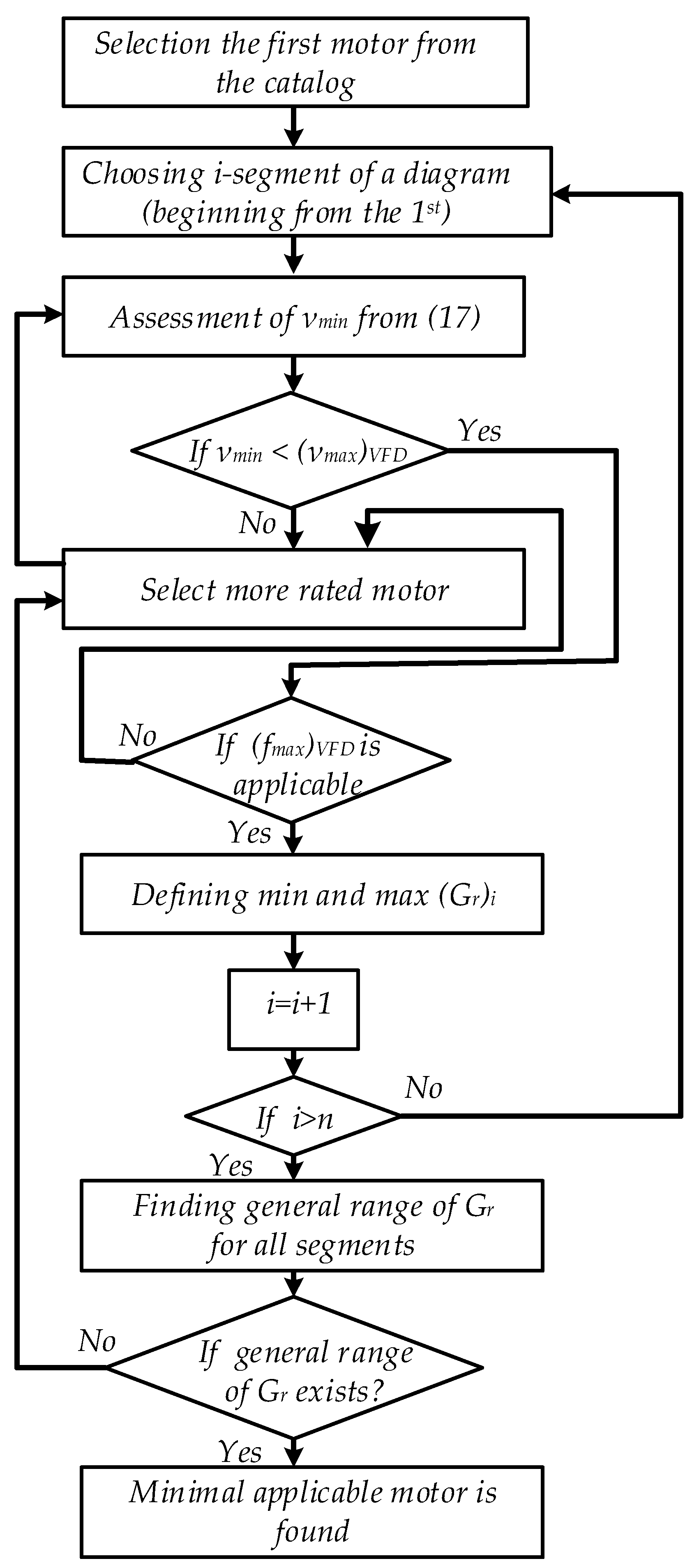
The motors located in the manufacturer’s catalog in ascending order of power are applicable for the task. However, the optimal motor is the one with the minimum size. Therefore, the first motor in the manufacturer’s catalog should be taken as the optimal solution, which satisfies Equation (5).

The proposed solution signifies a combinatorial optimization in which one parameter for the selection (gear ratio) should have a permanent value for the average driving cycle and therefore for the vehicle functionality. The two others (voltage magnitude and supply frequency) are permanently controlled. The possible gear ratio values must be selected at the first step of the solution.

2.3. Matching of AC Motor–Gearbox Coupling

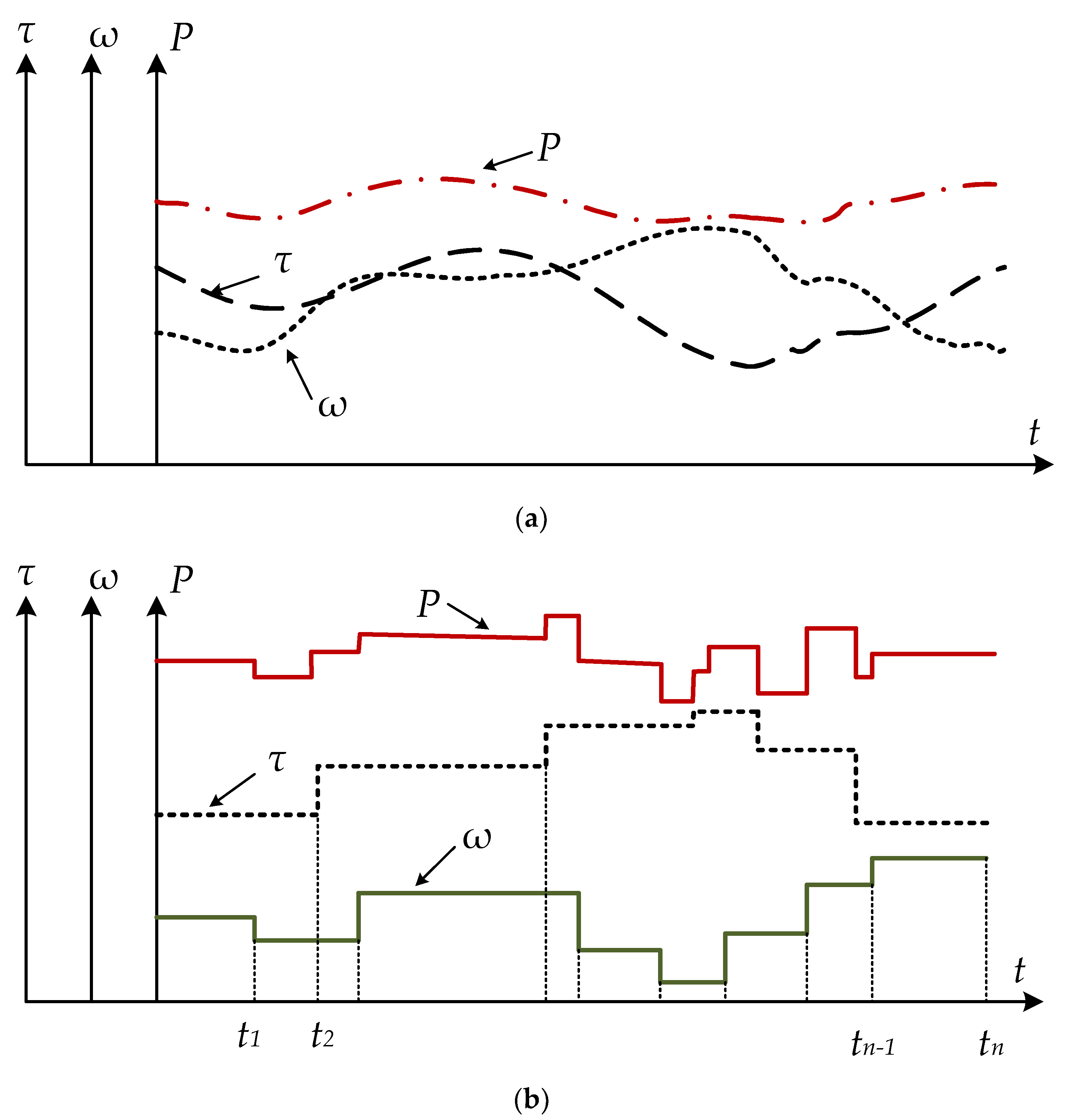
Considering a rapid and significant change of the required rotation velocity, torque, and driving power during the transportation cycle, the choice of an appropriate motor coupled with a gearbox represents an important challenge. Therefore, the approach based on the energy conservation law was chosen for the solution of this task. Thus, each segment of power required by vehicle is taken into consideration. A motor provides this power through a gearbox. The power needed in each driving segment is bigger than the net driving efforts because of the inevitable losses in a gearbox:

$$P_i=\frac{{\left(P_{d.c.}\right)}_i}{{\eta }_T}=\frac{{\omega }_i{\tau }_i}{{\eta }_T}$$

(6)

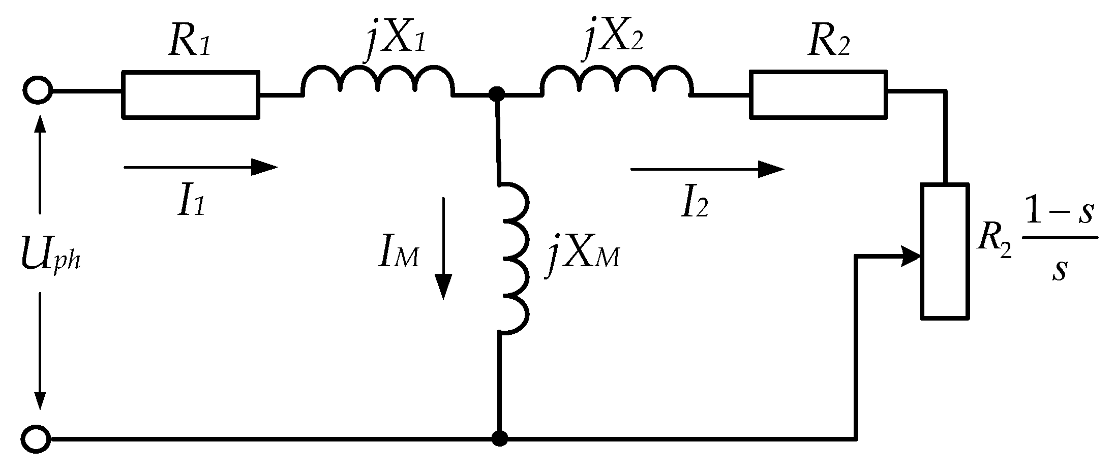
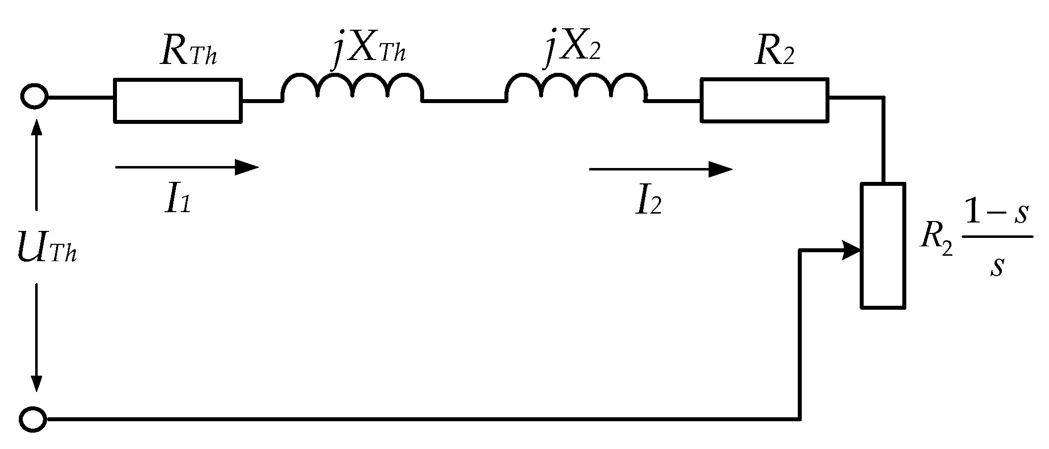
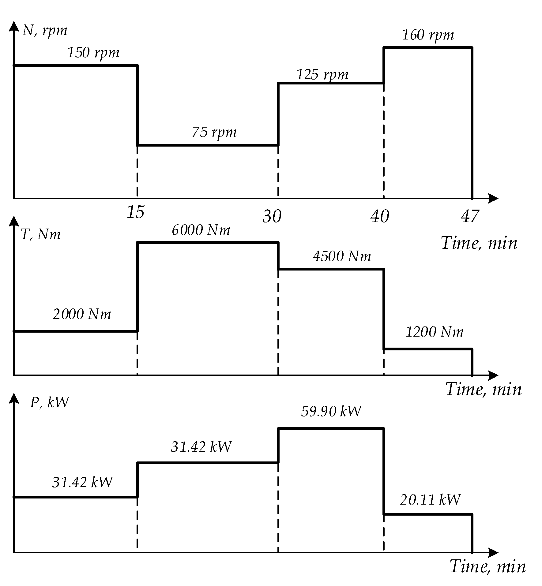
where ${\left(P_{d.c.}\right)}_i$ is the power of the driving efforts in the i_th time interval of the transportation diagram, ${\omega }_i$ is the rotation velocity in the i_th time interval, ${\tau }_i$ is the rotation velocity and torque in the i_th time interval, and ${\eta }_T$ is the efficiency of the gearbox. The ransportation diagram of a vehicle is a time-dependent function of the required torque vs. a driving velocity. It is challenging to select motor feeding parameters because of the uncertain choice. Numerous combinations of voltages and frequency can ensure the necessary power. Therefore, the AC motor parameters are analysed by the T-equivalent circuit (Figure 2). The equivalent circuit can be simplified for convenience with the Thevenin approach [40]. The simplified equivalent circuit is demonstrated in Figure 3.

Parameters $U_{Th}$, $R_{Th}$, and $X_{Th}$ are determined with the Kirchhoff circuit rules as follows:

$$\begin{gathered} U_{Th}=U_{ph}·abs\left(\frac{j{X}_M}{R_1+j\left(X_1+X_M\right)}\right)\approx U_{ph}\frac{X_M}{X_1+X_M}=U_{ph}\epsilon \\ {R}_{Th}=re\left(\frac{j{X}_M\left(R_1+j{X}_1\right)}{R_1+j\left(X_1+X_M\right)}\right)\approx R_1{\left(\frac{X_M}{X_1+X_M}\right)}^2 \\ {X}_{Th}=im\left(\frac{j{X}_M\left(R_1+j{X}_1\right)}{R_1+j\left(X_1+X_M\right)}\right)\approx X_1 \end{gathered}$$

(7)

wre $abs$, $re$, and $im$ operators signify absolute, real, and imagined magnitudes of the complex variables. Simplified expressions for $U_{Th}$, $R_{Th}$, and $X_{Th}$ are suitable for the calculations when the AC motor is supplied with nominal or slightly deviated voltages and frequencies.

Motor parameters (torque, velocity slip) vs. the applied voltage and frequency can be connected by the following expression [40]:

$$\begin{gathered} {\tau }_M=\frac{3U_{Th}^2{R}_2}{{\omega }_s}·\frac{s}{{\left(s{R}_{Th}+R_2\right)}^2+s^2{\left(X_{Th}+X_2\right)}^2} \\ {\omega }_s=\frac{2\pi f}{p},s=1-\frac{{\omega }_M}{{\omega }_s}. \end{gathered}$$

(8)

where ${\omega }_M$ and ${\omega }_s$ are synchronous and current motor rotation velocities, respectively.

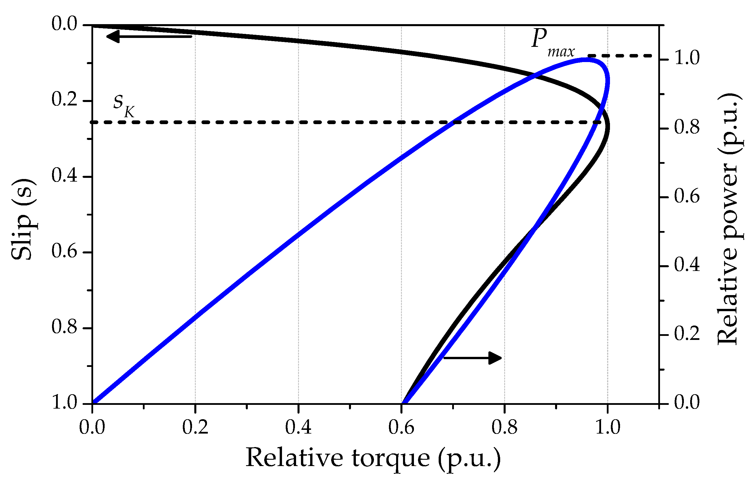
Motor power and other motor characteristics can be defined based on Equation (8). Figure 4 displays the typical AC motor parameters: critical slip ($S_K$) and maximum power ($P_{max}$). The critical slip is the velocity slip corresponding to the maximum achievable torque (${\tau }_{max}$). The power increases with motor loading until the power attains a maximum value ($P_{max}$), which should take place before the torque achieves a maximum value (${\tau }_{max}$). The motor power depends on the feeding voltage and current frequency. The specific relation of the motor power is influenced by individual VFD characteristics. Most VFDs provide a voltage that is proportional to the frequency ($V/f$ is constant). This relation provides the control of an AC induction motor with a constant magnetic flux and has well-known advantages such as maximum power and efficiency. Voltage increases with a frequency to some maximum limit ($U_{ph}<$ 450–480 V), which is restricted by the insulation breakdown capacity of a motor. After this point, even though the frequency increases, the voltage remains constant. The frequency range of a supplied voltage in VFD is also limited. The minimal frequency of the existing VFDs begins as usual from 5–10 Hz. The maximum frequency is limited in modern VFD below 80–100 Hz. This circumstance is defined by the maximal rotating ability of motor bearings and the ability of the conventional induction motors to operate at higher frequencies.

The power for the induction AC motor based on Equation (8) can be obtained as

$$\begin{gathered} {\mathit{P}}_{\mathit{M}}={\mathbf{\tau }}_{\mathit{M}}{\mathbf{\omega }}_{\mathit{M}}=\frac{3{\mathit{U}}_{\mathit{T}\mathit{h}}^2}{{\mathbf{\omega }}_{\mathit{m}\mathit{s}}}·\frac{{\mathit{R}}_2\mathit{s}\left(1-\mathit{s}\right){\mathbf{\omega }}_{\mathit{m}\mathit{s}}}{{\left(\mathit{s}{\mathit{R}}_{\mathit{T}\mathit{h}}+{\mathit{R}}_2\right)}^2+{\mathit{s}}^2{\left({\mathit{X}}_{\mathit{T}\mathit{h}}+{\mathit{X}}_2\right)}^2} \\ {\mathit{P}}_{\mathit{M}}=\frac{3{\mathit{U}}_{\mathit{T}\mathit{h}}^2}{{\mathit{R}}_2}·\frac{\left(1-\mathit{s}\right)\mathit{s}}{{\left(\mathit{s}\frac{{\mathit{R}}_{\mathit{T}\mathit{h}}}{{\mathit{R}}_2}+1\right)}^2+{\mathit{s}}^2{\left(\frac{{\mathbf{\omega }}_{\mathit{s}}}{{\mathbf{\omega }}_{\mathit{s}\mathit{n}}}\right)}^2{\left(\frac{{\mathbf{\omega }}_{\mathit{s}\mathit{n}}{\mathit{L}}_{\mathit{t}\mathit{o}\mathit{t}}}{{\mathit{R}}_2}\right)}^2} \\ {P}_M=\frac{3U_{Th}^2}{R_2}·\frac{{\upsilon }^2\left(1-s\right)s}{{\left(s\alpha +1\right)}^2+s^2{\upsilon }^2{\beta }^2} \end{gathered}$$

(9)

where p is the number of stator poles pairs; ($\alpha =R_{Th}/R_2$, $\beta ={\omega }_{sn}{L}_{tot}/R_2$, $\upsilon ={\omega }_s/{\omega }_{sn}$) are nondimensional parameters of resistance, reactance, and rotation velocity; ${\omega }_n$ is the nominal electrical frequency of the motor supply; and ${\omega }_{ms}$ is the mechanical synchronous motor speed (rad/s).

In the initial range for most of the existing VFDs, the supply voltage depends on the frequency and can be described functionally as $U_S=\phi \left(f_S\right)$. The linear approximation is accurate enough:

$$\begin{gathered} U_{ph}=U_0+K_2·f_S=U_0\left(1+\frac{f_{sn}{K}_2}{U_0}·\frac{f_s}{f_{sn}}\right) \\ {U}_{Th}=U_0\left(1+K_3\upsilon \right),\hspace{1em}{K}_3=\frac{f_{sn}{K}_2}{U_0} \end{gathered}$$

(10)

where $U_{ph}$. is the magnitude of phase voltage, which depends on the frequency supplied by VFD, $U_0$ is the initial voltage, $K_2$ is the aspect ratio between the voltage magnitude and frequency value ($f_s$), $f_{sn}$ is the nominal frequency of the AC motor, $\upsilon$. is the relative frequency ($f_s/f_{sn}$), and $K_3$ is the nondimensional coefficient.

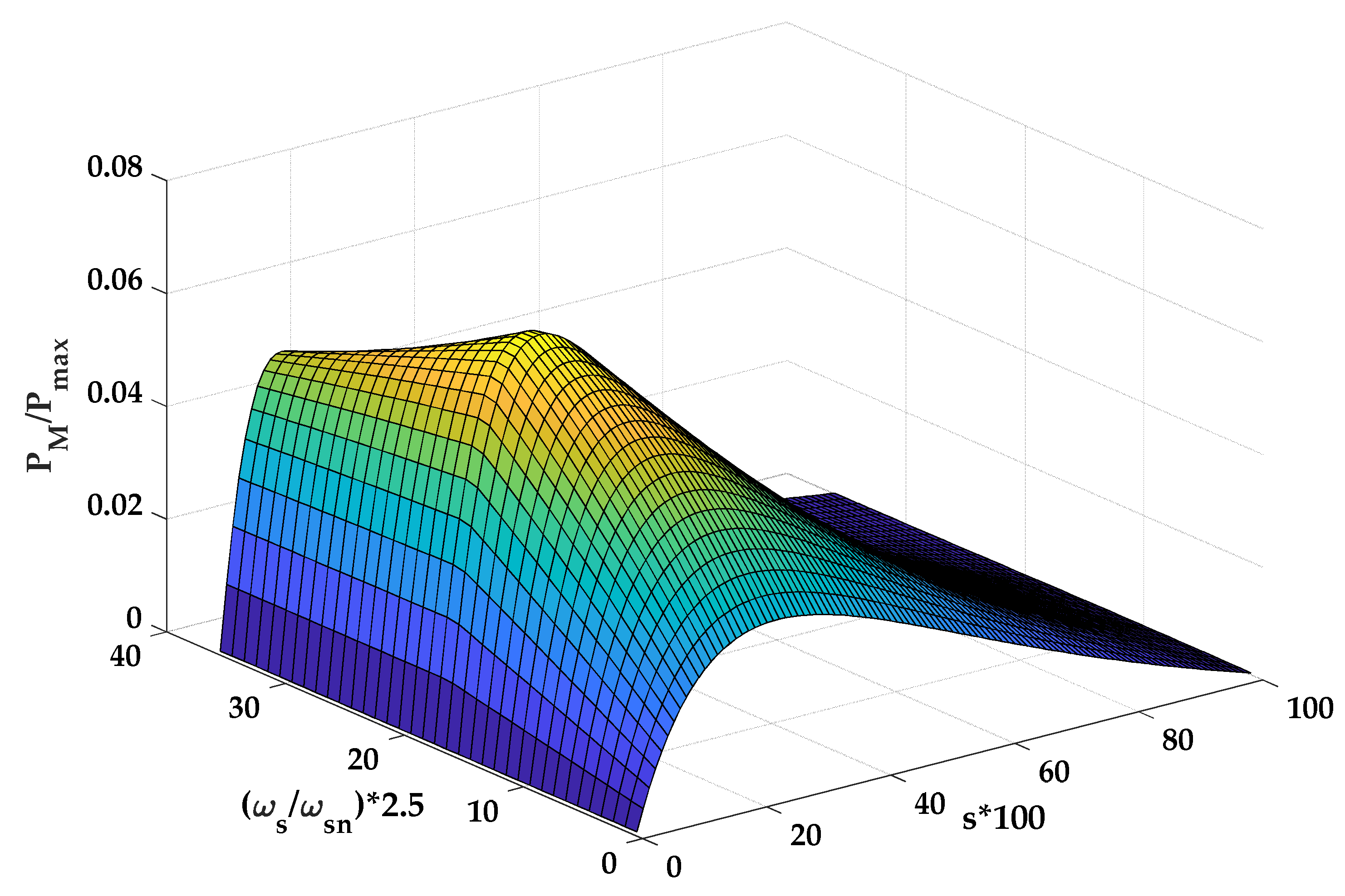
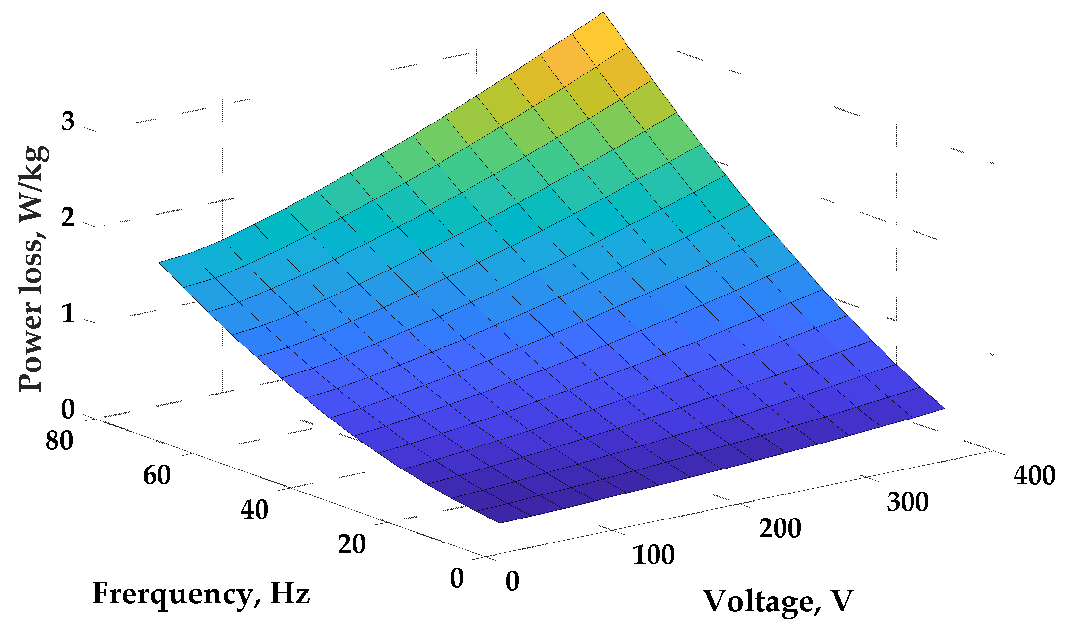
The supply voltage throughout the frequency range achieves a maximum permissible level of $U_s={\left(U_s\right)}_{max}$. As a result, the Thevenin voltage and achievable motor power do not remain constant. Accordingly, the motor power increases until ${\left(U_{Th}\right)}_{max}$ and then slowly decreases. A 3D graph of relative power vs. frequency and slip alterations for typical VFD is presented in Figure 5.

Equation (9) can be rearranged as follows:

$$\begin{gathered} \frac{P_M}{P_{max}}=\frac{s\left(1-s\right){\left(1+K_3\upsilon \right)}^2}{{\left(s\alpha +1\right)}^2+s^2{\upsilon }^2{\beta }^2}=\gamma . \\ {P}_{max}=\frac{3U_{ph}^2{\epsilon }^2}{R_2} \end{gathered}$$

(11)

A nondimensional equation that is valid for the ith interval of a loading diagram is compiled for the variable $s$:

$$\frac{P_{Mi}}{P_{max}}={\gamma }_i=\frac{s\left(1-s\right){\left(1+K_3\upsilon \right)}^2}{{\left(s\alpha +1\right)}^2+s^2{\upsilon }^2{\beta }^2}$$

(12)

After the simplification, a quadratic Equation (12) takes the form:

$$s^2\left[{\alpha }^2{\gamma }_i+{\beta }^2{\gamma }_i+{\left(1+K_3\upsilon \right)}^2\right]-s\left(2\alpha {\gamma }_i-{\left(1+K_3\upsilon \right)}^2\right)+{\gamma }_i=0$$

(13)

There are two possible solutions for $s$:

$$s_{1,2}=\frac{\left[{\left(1+K_3\upsilon \right)}^2-2\alpha {\gamma }_i\right]\pm \sqrt{{\left(1+K_3\upsilon \right)}^4-4{\gamma }_i\left(\alpha +1\right){\left(1+K_3\upsilon \right)}^2-4{\gamma }_i^2{\beta }^2}}{2\left[{\alpha }^2{\gamma }_i+{\beta }^2{\gamma }_i+{\left(1+K_3\upsilon \right)}^2\right]}$$

(14)

Two roots of $s$ should be real and positive. As a result, the determinant in Equation (14) should be positive, together with the positivity of the third member in Equation (13). These conditions ensure both positive roots of $s$ if

$${\left(1+K_3\upsilon \right)}^2-2\alpha {\gamma }_i>0\to \upsilon >\frac{\sqrt{2\alpha {\gamma }_i}-1}{K_3}$$

(15)

The requirement for the positivity of the determinant in Equation (14) is

$${\left(1+K_3\upsilon \right)}^4-4{\gamma }_i\left(\alpha +1\right){\left(1+K_3\upsilon \right)}^2-4{\gamma }_i^2{\beta }^2>0$$

(16)

The above equation shows bi-quadratic inequality for ${\left(1+K_3\upsilon \right)}^2$. After the arrangement, and considering positive conditions only, we arrive at

$$>\frac{\sqrt{2{\gamma }_i}\sqrt{\alpha +1+\sqrt{{\left(\alpha +1\right)}^2+{\beta }^2}}-1}{K_3}$$

(17)

The fulfillment of condition (17) automatically ensures inequality (15) as

$$\frac{\sqrt{2{\gamma }_i}\sqrt{\alpha +1+\sqrt{{\left(\alpha +1\right)}^2+{\beta }^2}}-1}{K_3}>\frac{\sqrt{2\alpha {\gamma }_i}-1}{K_3}$$

(18)

Equation (17) determines the lower applicable limit of frequency for the $i$-segment of a motor operation:

$$\begin{gathered} {\upsilon }_{min}\ge \frac{\sqrt{2{\gamma }_i}\sqrt{\alpha +1+\sqrt{{\left(\alpha +1\right)}^2+{\beta }^2}}-1}{K_3}\to {\left({\omega }_s\right)}_{min} \\ =2{\omega }_{sn}\frac{\sqrt{2{\gamma }_i}\sqrt{\alpha +1+\sqrt{{\left(\alpha +1\right)}^2+{\beta }^2}}-1}{K_3} \end{gathered}$$

(19)

The value of the minimum frequency should be well inside the frequency range of VFD. If this condition is not fulfilled, then a more powerful motor should be selected for consideration. If the condition of Equation (19) is satisfied, then the slip ($s$) has two positive roots. The smallest root should be chosen since only this causes stable motor functionality. The second positive root is bigger than the critical slip $s_K$ and cannot provide regular motor operation. Therefore, the solution for feasible slip is

$$s=\frac{\left[{\left(1+K_3\upsilon \right)}^2-2\alpha {\gamma }_i\right]-\sqrt{{\left(1+K_3\upsilon \right)}^4-4{\gamma }_i\left(\alpha +1\right){\left(1+K_3\upsilon \right)}^2-4{\gamma }_i^2{\beta }^2}}{2\left[{\alpha }^2{\gamma }_i+{\beta }^2{\gamma }_i+{\left(1+K_3\upsilon \right)}^2\right]}$$

(20)

Motor slip ($s$) ensures the required output power and depends on the VFD frequency. Slip tends to diminish during increases in frequency, as evidenced by a negative derivative of Equation (20). The obtained slip should ensure stable and reliable motor functionality. For this purpose, it must be 1.5–1.7 times less than the critical slip ($s_K$). The critical slip is represented by nondimensional variables ($\alpha$, $\beta$, $\upsilon$) as follows [40]:

$$s_K=\frac{R_2}{\sqrt{R_{Th}^2+X_{tot}^2}}=\frac{1}{\sqrt{{\left(\frac{R_{Th}}{R_2}\right)}^2+{\left(\frac{{\omega }_s}{{\omega }_{sn}}\right)}^2{\left(\frac{{\omega }_{sn}{L}_{tot}}{R_2}\right)}^2}}=\frac{1}{\sqrt{{\alpha }^2+{\upsilon }^2{\beta }^2}}$$

(21)

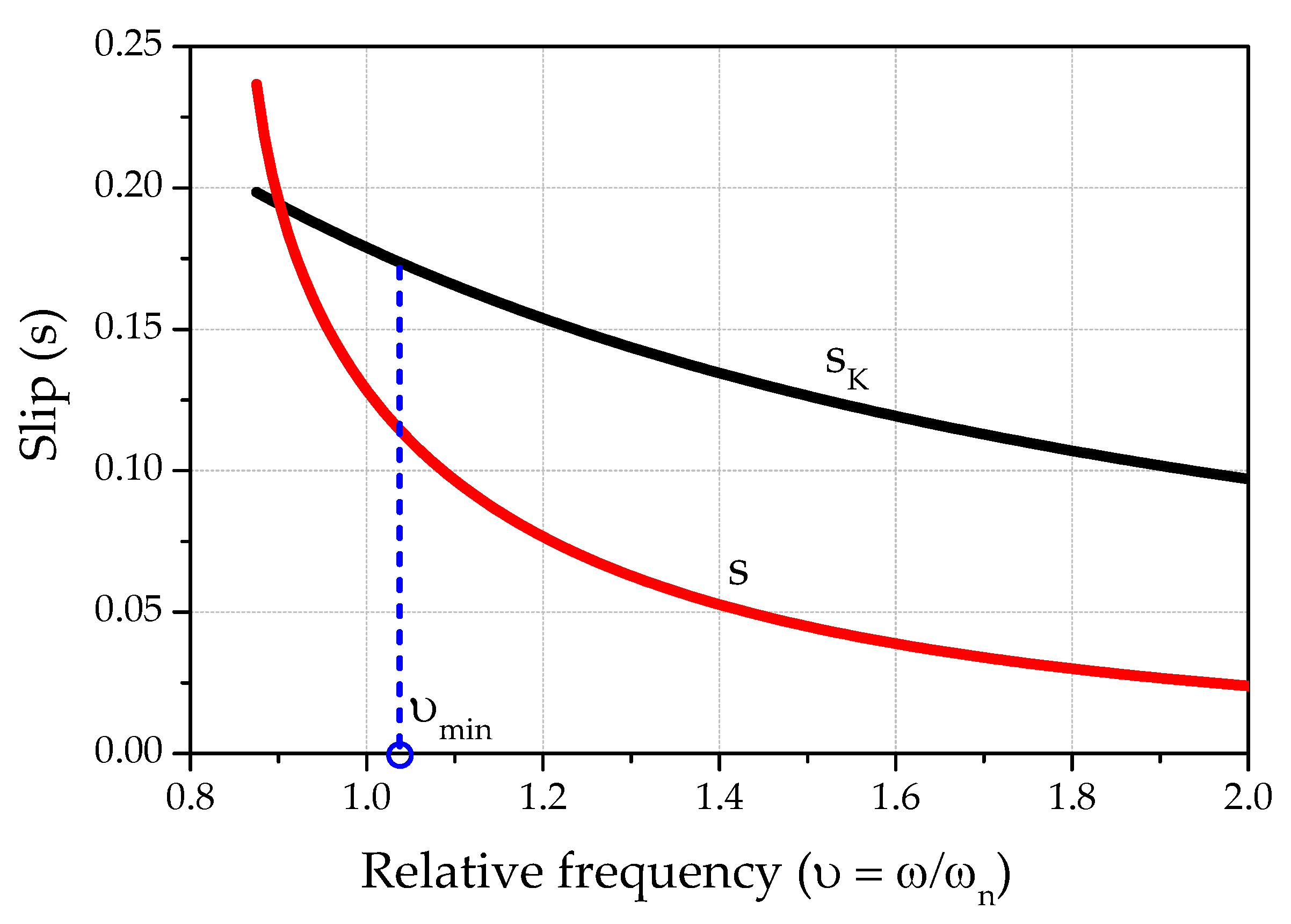
The relationship of $s$ and $s_K$ with the nondimensional parameter of frequency ($\upsilon$) is shown in Figure 6. The curves were obtained for $\alpha =$1.5, $\beta =$5, and $\gamma =$ 0.05. It is noticed that the $s_K$ value diminishes as frequency increases; however, with a lower rate. Therefore, to guarantee the required clearance between $s$ and $s_K$, a more rigorous inequality should be taken into consideration (Equation (22)).

This minimum applicable relative frequency (${\upsilon }_{min}$) can be found from the following difference:

$$\frac{\left[{\left(1+K_3\upsilon \right)}^2-2\alpha {\gamma }_i\right]-\sqrt{{\left(1+K_3\upsilon \right)}^4-4{\gamma }_i\left(\alpha +1\right){\left(1+K_3\upsilon \right)}^2-4{\gamma }_i^2{\beta }^2}}{2\left[{\alpha }^2{\gamma }_i+{\beta }^2{\gamma }_i+{\left(1+K_3\upsilon \right)}^2\right]}\le \frac{\left(0.55÷0.60\right)}{\sqrt{{\alpha }^2+{\upsilon }^2{\beta }^2}}$$

(22)

This equation can be solved with a numerical approach only because of its algebraic complexity. Importantly, it must be evaluated at the first step of the algorithm selection.

The VFD voltage control algorithm is significantly changed after the voltage attains the highest permissible value. As the voltage achieves maximum magnitude, it remains constant despite the increase in frequency. For many low-voltage VFDs, the maximum voltage limits are up to 450–480V. Equation (9) is modified to consider voltage permanence in this range of control:

$$\frac{{\mathrm{P}}_{\mathrm{Mi}}}{\left(\frac{3{\left(U_{Th}^2\right)}_{max}}{{\mathrm{R}}_2}\right)}={\gamma }_i^{*}=\frac{\left(1-\mathrm{s}\right)\mathrm{s}}{{\left(\mathrm{s}\mathsf{\alpha }+1\right)}^2+{\mathrm{s}}^2{\mathsf{\upsilon }}^2{\mathsf{\beta }}^2}$$

(23)

For steady motor operation, the solution of Equation (23) is

$$s=\frac{\left(1-2\alpha {\gamma }_i^{*}\right)-\sqrt{1-4{\gamma }_i^{*}\left(\alpha +1\right)-4{\left({\gamma }_i^{*}\upsilon \beta \right)}^2 }}{2\left[{\gamma }_i^{*}\left({\alpha }^2+{\upsilon }^2{\beta }^2\right)+1\right]}$$

(24)

Motor power decreases as frequency increases after the voltage achieves its maximum and remains constant. In principle, Equation (19) defines the maximum theoretically applicable frequency. Its relative value (${\upsilon }_{max}$) can be found according to the requirement for the expression under the square root to be positive:

$${\upsilon }_{max}\le \frac{1}{2{\gamma }_i^{*}\beta }\sqrt{1-4{\gamma }_i^{*}\left(\alpha +1\right)}$$

(25)

The vehicle motion control should ensure the required power ($P_{M_i}$) on each segment of the loading diagram for the entire frequency range if ${\upsilon }_{max}$[${\left({\omega }_s\right)}_{max}={\upsilon }_{max}{\omega }_{sn}$] is less than the upper-frequency limit of VFD. If this condition cannot be ensured, then a more powerful electric motor should be chosen for consideration. The lower relative (Equation (22)) and upper (Equation (25)) frequencies provide the calculation of achievable slips $s_{min}$ (Equation (14)) and $s_{max}$ (Equation (24)), respectively. Motor rotation velocities corresponding to these slips are calculated as

$${\left({\omega }_M\right)}_{min}=\frac{{\left({\omega }_s\right)}_{min}}{P}\left(1-s_{min}\right); {\left({\omega }_M\right)}_{max}=\frac{{\left({\omega }_s\right)}_{max}}{P}\left(1-s_{max}\right)$$

(26)

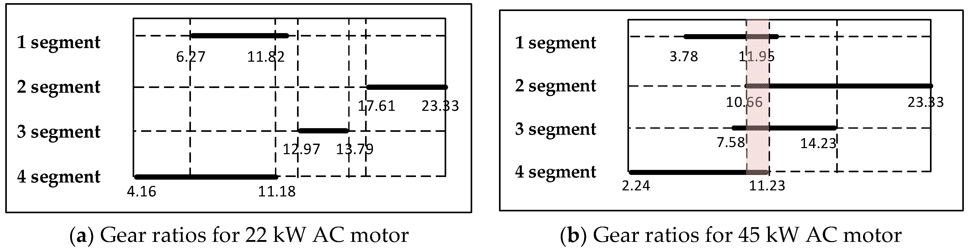
Finally, the gear ratio range ${\left(G_r\right)}_i$ for each $i$-segment of a loading diagram is as follows:

$${\left(G_r\right)}_i=\frac{{\left({\omega }_M\right)}_{min}}{{\left({\omega }_L\right)}_i}/\frac{{\left({\omega }_M\right)}_{max}}{{\left({\omega }_L\right)}_i}$$

(27)

The comparison of all ranges provides a generic span of gear ratios that is valid for the entire loading diagram. If a generic range is an empty set, then a more powerful motor should be selected.

2.4. Proposed Algorithm

Let us divide a driving diagram into several time segments with the motion parameters presented in

Table 1. Driving parameters of a loading diagram divided into n-segments.

Number of Segment (i)	Time Interval (s)	Wheel Rotation Velocity (rad/s)	Torque (Nm)	Pi (W)
1	t1	ω1	τ1	P1
2	t2	ω2	τ2	P2
…
n − 1	tn−1	ωn−1	τn−1	Pn−1
n	tn	ωn	τn	Pn

. The minimally applicable AC motor should be selected from a manufacturer catalog based on this table.

The proposed algorithm for the AC induction motor selection is shown in Figure 7. Firstly, the algorithm selects the first motor that seems to be suitable for this functionality. Let us follow the following rule of thumb: it is advisable to choose the first motor from the catalog with a nominal power equal to or slightly larger than the maximum power from $P_1-P_n$ divided by 3.5–4.0. Later, the range of valid gear ratios for each segment of a loading diagram should be found. The minimum frequency must be calculated previously to achieve this aim. After that, the minimal and maximal rotation velocities matching minimum and maximum frequencies are calculated. Later on, the minimal and maximal gear ratios for each segment are calculated. In the last stage, the general range of gear ratios is defined, which should not be an empty set. From this, all larger motors are valid for the optimal selection. The final choice should be determined by the comparison of the average motor losses with nominal ones.

2.5. Determination of AC Motor Losses

The efficiency estimation of AC induction motors is explicitly based on the mechanical, core (ferromagnetic), and resistive losses. In this work, total losses were chosen for the optimization of the motor–gear coupling in a drive system.

2.5.1. Resistive Losses in Induction Motor

The resistive losses are estimated using the equivalent circuit of the AC motor (Figure 2). Firstly, the equivalent circuit parameters should be found for the optimal motor selection and included in the motor catalog and datasheets. Resistive loss is calculated as

$$\mathsf{\Delta }{P}_{Cu}=3\left(I_1^2\mathsf{\Delta }{R}_1+I_2^2\mathsf{\Delta }{R}_2\right)$$

(28)

Current magnitudes ($I_1^{}$, $I_2^{}$) are calculated for the required working point. Output motor characteristics (torque and speed) are calculated with the simplified Thevenin equivalent circuit (Figure 3). The AC motor feeding from VFD inevitably requires the use of precise formulations for $U_{Th}$, $R_{Th}$, and $X_{Th}$. Firstly, it relates to the calculation of resistive losses. The skin-effect phenomenon influences the ohmic conductivity of motor windings. Let us consider a low current frequency in the rotor circuit due to the small slip of rotor velocity (less than 1–3%). The skin-effect influence can be considered for the stator windings only, and it can be neglected for rotor windings. Figure 8 shows the experimental setup for the resistance measurements of stator windings. Measurements were carried out on an induction motor with the values of 1 kW and 230/400 V by the RLC meter of BK Precision Co. [41]. Measurements results are presented in Figure 9.

The deviation of resistance in all three stator circuits is less than 0.2%, showing good winding symmetry and equality. The stator resistance for any AC induction motor at an arbitrary frequency $f$ is calculated as

$$R_f=R_{50Hz}\left[1+1.86·{10}^{-3}\left(f-50\right)\right]$$

(29)

where $R_{50Hz}$ is the equivalent stator resistance ($R_1$ in Figure 2) at the working motor temperature, which is obtained from the manufacturer’s datasheets. $R_f$ is the stator resistance for the current frequency supply. The measurements for stator reactance show its relative constancy (116–135 mH) in a wide range of applicable supply frequencies of 20–100 Hz. Therefore, all reactances can be assumed to be constant values in the further calculation of motor parameters. The current ($I_1$, $I_2$) can be found from the equivalent circuit (Figure 2) based on the previously calculated variables $U_{Th}$, $s$, and ${\omega }_s$ (in Section 2.4). However, the correction for parameters ($R_1$, $X_M$, $X_2$) should be done according to the applied frequency during the calculation. Once currents are determined, resistive losses for the chosen gear ratio can be calculated.

2.5.2. Mechanical and Core Losses

Despite having different natures, mechanical and core losses are estimated altogether under the consideration of the relative constancy of the induction motor velocity for the same feeding parameters of voltage and frequency. However, these losses act differently from the frequency and voltage alteration generated by VFD. This should therefore be considered. The mechanical and core losses are estimated with the concepts of constant and variable losses due to a nominal motor feeding-rayed voltage and frequency [39]. Corresponding coefficients $K_1$ and $K_2$ are used to determine constant and variable losses. Their values can be found through the formulation of nominal and current power losses ($\mathsf{\Delta }P$, $\mathsf{\Delta }{P}_n$) vs. nominal and current motor outcomes, $P_n$ and $P$:

$$\mathsf{\Delta }P=\mathsf{\Delta }{P}_n\left(K_1+K_2{\left(\frac{P}{P_n}\right)}^2\right)$$

(30)

Coefficients $K_1$ and $K_2$ are calculated with motor efficiency for a full and half-loaded AC motor (${\eta }_n$ and ${\eta }_{50\%}$) by the following equations:

$$\begin{gathered} \mathsf{\Delta }{P}_n=P_n\frac{1-{\eta }_n}{{\eta }_n} \\ \mathsf{\Delta }{P}_{50\%}=\frac{P_n}{2}·\frac{1-{\eta }_{50\%}}{{\eta }_{50\%}} \\ {K}_2=\frac{4}{3}\left(1-\frac{\mathsf{\Delta }{P}_{50\%}}{\mathsf{\Delta }{P}_n}\right) \\ {K}_1=1-K_2 \end{gathered}$$

(31)

Mechanical and core losses during motor feeding from VFD should be split and calculated independently. However, in this case, the coefficient $K_{mech}$ must be equal to that calculated from Equation (33). Mechanical losses can be estimated as proportionally dependent on rotation velocity ${\omega }_m$:

$$\mathsf{\Delta }{P}_{mech}=K_{mech}·{\omega }_m$$

(32)

The coefficient $K_{mech}$ is 40–50%% of coefficient $K_1$, since for the nominal motor feeding (voltage, frequency), pure mechanical loss is approximately half of the constant loss. Therefore,

$$K_{mech}=\frac{\left(0.4-0.5\right)K_1·\mathsf{\Delta }{P}_n}{{\omega }_n}$$

(33)

where ${\omega }_n$ is the rated motor velocity. Core losses during voltage and frequency alterations should be assessed independently by modified or generalized Steinmetz expressions [40]:

$$\mathsf{\Delta }{P}_C=K_C{B}^{\alpha }{f}^{\beta }$$

(34)

Coefficients $\alpha$ and $\beta$. for the sinusoidal excitation were taken from [42,43], and their magnitudes are approximated based on the presented literature data as

$$\alpha =2.181,\beta =-0.89+1.25B^{-0.2}{f}^{0.2}$$

(35)

Coefficient $K_C$ can be found according to the weight of a motor stator:

$$K_C=W_{st}·2.476$$

(36)

where $W_{st}$ is the weight of the motor stator.

The weight of a motor stator can be estimated as a portion of the total motor mass: 39–42% for the steel case and 45–48% for the aluminum case. Taking into consideration Equations (31)–(36) for the core losses vs. frequency and voltage alterations,

$$\mathsf{\Delta }{P}_C=K_C{U}^{2.181}{f}^{-0.89+1.25U^{-0.2}{f}^{0.2}}$$

(37)

Here, we considered that the supply voltage could be used to calculate induction ($B$) as follows:

$$B=\frac{U}{4.44A_{st}{N}_{ }f}$$

(38)

where $A_{st}$ is stator area, $N$ is the turn number, and $f$ is frequency. A typical 3D plot for the relative core losses is shown in Figure 10.

3. Results

The selection procedure for the demonstration of the submitted methodology is demonstrated in the following example. The given loading diagram is presented in Figure 11 and

Table 2. Loading diagram of a vehicle.

Time-Interval (i)	Segment Time (min)	Rotation Velocity (rpm)	Rotation Velocity (rad/s)	Torque (Nm)	Power (W)	Motor Power (W)
1	15	150	15.71	2000	31,420	35,705
2	15	75	7.85	6000	47,100	53,522
3	10	125	13.09	4500	58,905	66,938
4	17	160	16.75	1200	20,110	22,852

.

For simplicity, a loading diagram was chosen to consist of only four-time intervals. A loading diagram can be divided into many time intervals that will ensure more precise motor selection. It is worth pointing out that the dependence of the load diagram from the type of the vehicle and its exploitation characteristics.

To demonstrate the submitted approach, the group of six consecutive low voltage, AC induction motors (380 V, 50 Hz, $n_{synch}=$ 1500 rpm (50π rad/s)) from the manufacturer’s catalog was selected (

Table 3. Possible AC motors for optimal selection.

${\mathit{P}}_{\mathit{n}}\left(\mathbf{kW}\right)$	n (rpm)	${\mathit{I}}_{\mathit{n}}\left(\mathbf{A}\right)\left(400\mathbf{V}\right)$	Efficiency (%)	P.F. (p.u.)	${\mathit{T}}_{\mathit{n}}\left(\mathbf{Nm}\right)$	${\mathit{T}}_{\mathit{m}\mathit{a}\mathit{x}}$$/{\mathit{T}}_{\mathit{n}}$	Weight (kg)
22	1468	39.3	91.2	0.89	143	2.4	184
30	1472	53.1	92.1	0.89	195	2.2	286
37	1476	67.6	92.2	0.86	239	2.1	338
45	1477	80.9	92.5	0.87	291	2.3	358
55	1475	98.7	92.9	0.87	356	2.4	449
75	1482	133.6	94	0.86	483	2.2	535

). The optimal motor should be chosen for the represented loading diagram (Table 2).

The Thevenin equivalent circuit parameters of each motor are summarized in

Table 4. Parameters of Thevenin equivalent circuits.

${\mathit{P}}_{\mathit{n}}\left(\mathbf{kW}\right)$	${\mathit{R}}_1\left(\mathsf{\Omega }\right)$	${\mathit{R}}_2\left(\mathsf{\Omega }\right)$	${\mathit{X}}_1$$= {\mathit{X}}_2\left(\mathsf{\Omega }\right)$	${\mathit{X}}_{\mathit{m}}\left(\mathsf{\Omega }\right)$	${\mathit{L}}_{1 }$$= {\mathit{L}}_2\left(\mathbf{mH}\right)$	${\mathit{L}}_{\mathit{m}}\left(\mathbf{mH}\right)$
22	0.4412	0.4044	1.211	39.15	3.855	124.62
30	0.8521	0.2471	0.6482	31.76	2.063	101.10
37	0.7196	0.1671	0.6975	22.55	2.220	71.78
45	0.3803	0.1379	0.5914	19.12	1.883	60.86
55	0.3877	0.1198	0.5069	16.39	1.614	52.17
75	0.2291	0.065	0.3563	11.52	1.134	36.67

.

For the control, motors with V/f control (VFD of Danfoss Co. [44]) were chosen. The output VFD voltage ($V$) is expressed as

$$\begin{gathered} V=150+6.2·f\hspace{1em}\mathrm{for}f<55 Hz \\ V=490\hspace{1em}\mathrm{for}55Hz\le f\le 60 Hz \end{gathered}$$

(39)

For each motor, gear ratio ranges were calculated according to Equation (19), and all four segments of the loading diagram are represented in

Table 5. Gear ratio ranges applicable for all AC motors.

Gear Ratio
Motor Size (kW)	1		2		3		4
	Min	Max	Min	Max	Min	Max	Min	Max
19	7.45	11.83	20.14	23.25	X	X	4.94	11.18
22	6.27	11.82	17.61	23.33	12.97	13.79	4.16	11.17
30	5.34	11.91	14.65	23.66	10.47	14.08	3.42	11.22
37	5.08	11.93	14.25	23.73	10.20	14.16	3.22	11.22
45	3.78	11.95	10.66	23.82	7.58	14.24	2.24	11.23
55	3.46	11.96	9.88	23.86	7.06	14.27	1.99	11.24
75	2.16	11.98	6.73	23.94	4.97	14.34	1.00	11.24

.

The analysis of the selected motors shows the principal possibility of applying motors beginning from $P_n=$ 22 kW and further. The lighter motor of 18.5 kW cannot ensure the entire loading diagram and drive vehicle in the third segment. Only more powerful motors can provide all segments of a driving diagram. However, the AC motors rated by 22 kW, 30 kW, and 37 kW have no common range of gear ratios in the overall range. Therefore, these motors cannot be applied for the entire loading diagram with the idem gear ratio. The overall gear ratio ranges are illustrated in Figure 12a,b. The assessment of the overall gear ratios (

Table 6. Common affordable gear ratio for AC motors.

Motor Size (kW)	Common Gear Ratio		Total Losses (W)		Nopt (n:1)
	Min	Max	Real	Nom
19	No	No	–	–	–
22	No	No	–	–	–
30	No	No	–	–	–
37	No	No	–	–	–
45	10.66	11.23	4384	3649	11.15:1
55	9.88	11.24	4707	4203	11.03:1
75	6.73	11.24	4299	4787	9.31:1

) shows that a common range exists only for 45 kW and bigger AC motors.

As expected, the range of the overall gear ratio grows with increasing motor power. In the next step, power losses are estimated for the final selection of the optimal AC motor. Each interval of gear ratios is divided into several evenly distributed magnitudes. Further, torque and rotation velocity parameters from a loading diagram are reflected as the required motor velocity and torque. The voltage and frequency magnitudes of VFD are defined based on the necessary motor parameters. This provides an estimation of the motor current and then mechanical, winding resistance, and core losses. The gear ratio ensuring minimal average losses in all segments of a loading diagram is defined as the best solution for a chosen motor. Despite the principle possibility of motors rated from 37 kW to ensure loading diagram, the 75 kW AC motor only shows minimal real losses that are less than the nominals. Therefore, this is the optimal selection for the chosen loading diagram.

4. Discussion

This work represents the solution to the optimal selection of an AC induction motor fed by VFD which is applicable to work in the driving system of an electrified vehicle with some chosen loading diagrams. For the first time, the motor selection for an electrified vehicle was carried out to find the optimal motor–gearhead combination. This methodology ensures an arbitrary loading diagram with minimal losses and weight of the AC motor. The optimal choice requires both the selection of a motor and an optimally matching gearhead defined by its gear ratio considering the functionality of VFD. The optimal combination of the AC motor–gearhead-load is based on minimizing drive system losses and choosing the minimal motor with an average efficiency less than the nominal one from a manufacturer’s catalog. An original AC induction motor estimation algorithm that can be used for a given loading diagram was developed. A special mathematical procedure describing the motor functionality parameters (e.g., motor losses) and gearhead ratio was created with the equivalent circuit on the Thevenin approach. The example of a motor-gearhead selection was demonstrated for some arbitrarily chosen loading diagrams. The represented instance shows the importance of VFD with a wide frequency and voltage range for minimizing average losses and including a smaller AC motor in the drive system.

This study paves the way for future research work in this area, including the variant of a driving system with a controllable gearhead with either continuously variable or several ranges of stepped transmission ratios.

5. Conclusions

The analysis of the proposed approach for the optimal selection of an AC motor in the driving system of an electrified vehicle illustrates the importance of the correct choice of the AC motor–gear ratio combination for minimizing losses and decreasing motor weight. It is proposed that this optimal selection should be evaluated by comparing the average AC motor losses during the driving cycle diagram with those determined by nominal motor parameters. The calculation of motor losses (mechanical, ferromagnetic core, and resistive) is assessed with an equivalent Thevenin motor circuit, which is estimated before motor selection. Based on the equivalent circuit, the feasible range of gear ratio magnitudes for each segment of a loading diagram is calculated. Further, the general common ratio ranges for a specific motor applicable for the entire loading diagram are established. Only AC motors with a common ratio range for the total loading diagram are taken into consideration. Later, the optimal ratio magnitude inside a common range ensuring minimum average motor losses is found. Finally, the first AC motor from the manufacturer guaranteeing average losses not more than the nominal losses is selected as an optimal choice. The proposed algorithm can be fulfilled by programming software, making the selection procedure more suitable and electric vehicles more reliable and sustainable.