Evaluating the Dynamic Energy Production Efficiency in APEC Economies

Abstract

This study introduces the translation adjustment model of Seiford and Zhu (2002) into dynamic DEA models to measure and analyze the dynamic energy efficiency of Asia-Pacific Economic Cooperation (APEC) economies from 2010 to 2014. The APEC economies are divided into annual energy and overall energy efficiency ratings, and improvement directions are proposed for the different variables. With the proposal of magnitude, this study discusses the changes in intertemporal conversion variables and proposes suggestions for improvement. Finally, this study analyzes the implications of energy investment and the efficiency policies of APEC economies. The results show that economies with the lowest overall energy efficiency ratings have great potential for improvement. Reducing capital stock, labor, fossil fuel consumption, and CO₂ emissions while increasing GDP can increase energy efficiency ratings. However, economies do not want to reduce the state’s capital stock, and labor and population birth adjustments are difficult. Energy efficiency can only start by adjusting the consumption of fossil fuels, CO₂ emissions, and GDP. The results indicate that to improve energy efficiency and reduce fossil fuel consumption and CO₂ emissions, economies are expected to increase their GDP unless they enact cuts through policy and technical approaches, appropriately adjust their energy policies, and actively develop new energy technologies to effectively reduce CO₂ emissions and achieve optimal energy efficiency.

1. Introduction

International attention on the effects of excessive energy consumption began with the United Nations Framework Convention on Climate Change (UNFCCC), as adopted by the United Nations Headquarters in 1992. (The United Nations Framework Convention on Climate Change: the purpose is to stabilize the concentrations of greenhouse gases in the atmosphere in order to adapt the climate system to climate changes without any human interference and to take food production and economic development into account.)Then, it continued to the Kyoto Protocol (Kyoto Protocol: the creation of detailed regulations and legally enforceable reduction targets, including how to mitigate and combat climate change, and promotion of the “Kyoto Protocol” to become international law are the first steps to reverse global climate change), which represents the supplementary terms of the UNFCCC and was passed in Kyoto, Japan, in 1997, and to the Paris Agreement (Paris Agreement: to keep the earth’s temperature rise within a maximum of 2 °C, as compared with the temperature in preindustrial times, and to strive to achieve the abovementioned temperature rise standard and continue to reduce to the target of within 1.5 °C. Unlike the Kyoto Protocol, the Paris Agreement extends the emission reduction obligations to China and India and requires developed countries to provide climate change funds to help developing countries reduce their carbon dioxide emissions and to be capable of facing the consequences resulting from global climate change. It also makes all countries set their own emission reduction targets over a five-year cycle), which was passed at the United Nations Climate Summit in 2015. It is known that energy issues are closely related to world climate change issues, food issues, population issues, and water resources. (The eight major issues discussed at the 2016 World Economic Forum (WEF) indicated that climate change is the most serious global problem at present, and failure to efficiently deal with climate change is the biggest threat to the global economy (WEF, 2016). The 2017 Climate Vulnerable Forum (CVF) also explicitly indicated that the main cause of global climate change is global temperature warming, which comes from the excessive emissions of carbon dioxide, and such massive greenhouse gas emissions arising from fossil fuel cause an increase in the average global temperature, melt the ice caps, and cause extreme weather, drought, and rising sea levels. If climate change cannot be dealt with efficiently, hundreds of millions of people may die by 2030, and the annual global gross domestic product will decrease.) Therefore, ways to save energy, improve energy efficiency, develop green energy, and reduce carbon dioxide emissions have long been important issues of international concern.

According to the data on carbon dioxide emissions, as collected by CDIAC for the United Nations, and the gross domestic product (GDP) statistics collected in the United Nations database (UN data), in 2015, the world’s top 10 carbon dioxide emitters accounted for 67.07% of the world’s total emissions, as shown in

Table 1. The 10 economies with the top carbon dioxide emissions worldwide in 2015.

Ranking	Carbon Dioxide Emissions (KMT)	Percentage of World (%)	GDP Ranking	Remark
World	36,061,710	100%	-	-
1 China	10,641,789	29.51%	2	APEC member
2 the U.S.	5,172,338	14.34%	1	APEC member
3 the E.U.	3,469,671	9.62%	-	-
4 India	2,454,968	6.81%	7	-
5 Russia	1,760,895	4.88%	12	APEC member
6 Japan	1,252,890	3.47%	3	APEC member
7 German	777,905	2.16%	4	-
8 Iran	633,750	1.76%	29	-
9 South Korea	617,285	1.71%	11	APEC member
10 Canada	555,401	1.54%	10	APEC member

Source: U.S. Department of Energy Carbon Dioxide Information Analysis Center (CDIAC, https://cdiac.ess-dive.lbl.gov/trends/emis/top2014.tot (accessed on 29 June 2021)), United Nations database (UNDATA (accessed on 29 June 2021)).

, and their gross domestic products rank among the highest in the United Nations. Six of these countries are APEC economies: China, the United States, Russia, Japan, Korea, and Canada. Moreover, China ranked first in terms of global carbon dioxide emissions in 2015, accounting for 29.51% of total global emissions.

The Asia-Pacific Economic Cooperation (APEC) (The official website of Asia–Pacific Economic Cooperation (APEC): https://www.apec.org/ (accessed on 29 June 2021)) is one of the most significant multilateral official economic cooperation forums in the Asia Pacific region, and there are a total of 21 participant economies: The United States, Russia, China, Japan, Canada, Singapore, Australia, Taiwan, Brunei, Chile, Hong Kong, Indonesia, Korea, Malaysia, Mexico, New Zealand, Peru, Papua New Guinea, the Philippines, Thailand, and Vietnam. It cannot be ignored that the total population of APEC economies accounts for 40.00% of the global population, their gross domestic products account for nearly 55.00% of the global total, and their total trades account for nearly 44.00% of the global total. In terms of geographical range, overall economic strength, and organizational activities, the consensus reached by APEC has a substantial influence on global economic and trade policies, as well as norms.

As shown in Table 1, there were a total of 6 APEC economies among the world’s top 10 carbon dioxide emitters in 2015, as previously mentioned. Among them, China is the largest energy demander, and in 2015, its emissions accounted for 29.51% of the global total and ranked first, while its gross domestic product ranked second in the United Nations. The United States is a large energy consumer and importer, and in 2015, its emissions accounted for 14.34% of the global total and ranked second, and its gross domestic product ranked first in the United Nations. Russia is the largest oil and natural gas exporter in the world, and in 2015, its emissions accounted for 4.88% of the global total and ranked fifth, and its gross domestic product ranked twelfth in the United Nations. Japan is currently the fifth-largest energy consumer and the second-largest energy importer in the world, and in 2015, its emissions accounted for 3.47% of the global total and ranked sixth, and its gross domestic product ranked third in the United Nations. Korea is the eighth largest energy consumer in the world, and in 2015, its emissions accounted for 1.71% of the global total and ranked ninth, and its gross domestic product ranked eleventh in the United Nations. Canada is an important petrochemical energy producer, and in 2015, its emissions accounted for 1.54% of the global total and ranked tenth, and its gross domestic product ranked tenth in the United Nations. Environmental protection and proper resource allocation have long been a focus issue of international concern, and energy efficiency is the core of this issue. As shown in Table 1 and

Table 2. Economies belonging to APEC with the highest carbon dioxide emissions in 2015.

Economy	Energy Situation	Ratio of CO2 Emissions to the World (%)	GDP (Million Dollars)
China	The largest energy user	29.51%	11,158,857
The U.S.	Higher energy consumption and imports	14.34%	18,036,648
Russia	The world’s largest exporter of oil and gas	4.88%	1,365,865
Japan	The world’s fifth-largest energy consumer and the second largest energy importer	3.47%	4,383,076
South Korea	The world’s eighth-largest energy consumer	1.71%	1,382,764
Canada	Important producer of petrochemical energy	1.54%	1,552,807
Percentage of the world		55.45%	45.15%

Source: U.S. Department of Energy Carbon Dioxide Information Analysis Center (CDIAC, https://cdiac.ess-dive.lbl.gov/trends/emis/top2014.tot (accessed on 29 June 2021)), United Nations database (UNDATA (accessed on 29 June 2021)).

, in 2015, the total gross domestic products of six APEC economies, China, the United States, Russia, Japan, Korea, and Canada, accounted for 45.15% of the global total, and their carbon dioxide emissions accounted for 55.45% of the global total, which was more than half of the total global emissions. These notable statistical data once again stress the necessity and importance of evaluating the energy efficiency of APEC economies.

All economies pursue economic development, so is it possible to look back and consider the living environment that has been created for the next generation? This research collects the data of APEC economies from 2010 to 2014 and uses the dynamic DEA model to evaluate and analyze the energy efficiency rankings of 20 economies based on their CO2 emissions calculated from fossil fuels. The targets of this research are as follows: (1) discussing the annual and overall energy efficiency of APEC economies; (2) making suggestions for improvement directions and ranges of different variables; (3) exploring changes in the intertemporal conversion variables of APEC economies and suggestions for improvement; (4) analyzing the energy inputs and efficiency policy implications of APEC economies.

Over the past several decades, many studies have focused on the themes of energy and the environment to find appropriate solutions balancing economic growth and environmental protection, energy consumption and CO₂ emissions (Pittman [1], Weber and Domazlicky [2], Zofio and Prieto [3]). Among these, DEA models have been applied to measure the energy efficiency [4,5,6,7,8,9,10,11,12,13,14,15,16,17,18,19,20,21,22,23,24,25,26,27,28,29]. Studies related to energy efficiency usually take undesirable outputs into account and assess the value of energy efficiency through various DEA models (Pittman [30], Fär, Grosskopf, Lovell, and Pasurka [31], Färe, Grosskopf, and Kokkelenberg [32], Scheel [33], Pasupathy [34]). There are two main methods to analyze undesirable outputs: 1) considering them as weak disposable (WD) variables in their original forms (Färe and Grosskopf [35,36,37]) and 5) treating them as strong (free) disposable (SD) variables in their different forms, such as in the form of their additive inverse or in the form of their reciprocals (see AlirenzaAmirteimoori, Kordrostami and Sarparast [38], Seiford and Zhu [39], Lovell [40], Athanassopoulos and Thanassoulis [41], Arcelus and Arocena [42]).

Nevertheless, one limitation of such research is that they evaluated the efficiency of bad outputs within cross-sectional data but not time-series data. The changes in carry-over variables that persist during the sample period were not considered. To be more specific, previous studies usually applied traditional DEA models to evaluate the production efficiency and technical efficiency of decision-making units (DMUs) during a certain period of time in a static way, while if we adopt the assumption of static optimization, there may be inefficient biased measurements. Therefore, in the long term, the quasi-fixed inputs may not be allocated efficiently or adjusted to optimal levels, according to the results of Nemoto and Goto [43]. Moreover, when considering some terms with intertemporal effects to assess overall efficiency, the interrelationship between successive periods must be analyzed dynamically (Kao [44]). It is necessary for us to establish a dynamic DEA model to calculate the energy efficiency of 20 APEC economies.

Sengupta [45] and Färe and Grosskopf [6] mainly contributed to the development of the dynamic data envelopment analysis model. Sengupta [45] showed a dynamic DEA model by introducing the adjusted cost method to analyze the risk and output fluctuation of a dynamic production frontier when the shadow value of quasi-fixed input and its optimal path are incorporated into the analysis of linear programming. Färe and Grosskopf [3] formulated different intertemporal variables and input them into actual multioutput production processes for various periods. Since then, much research has followed and developed dynamic DEA models [46,47,48,49,50,51,52]. Tone and Tsutsui [53] connected two consecutive periods by merging the carry-over variable, establishing a slack-based model for measuring period and overall efficiencies. Jafarian-Moghaddam and Ghoseiri [54] built a fuzzy dynamic multi-objective DEA model to evaluate railway efficiency performance. Soleimani-damaneh [55] developed a new technique to estimate the return on a scale using the dynamic DEA model to obtain the advantages of the algorithm. Based on the quarterly data of the Zagreb Stock Exchange, Tihana [56] used a dynamic slack-based measure (SBM) DEA model to assess the relative efficiency during the period 2009–2012. Sueyoshi et al. [57] evaluated the environmental performance of coal-fired power plants in the United States from 1995 to 2007 by using dynamic DEA window analysis at the time-shifting front.

Our study aims to respond to the results estimated by Seiford and Zhu [39], which use CO₂ emissions as undesirable output and view real GDP as a carry-over variable in dynamic DEA models (Tone and Tsutsui [53]). The method commonly used in the literature for assessing efficiency tends to produce overestimated efficiency scores when the essence of dynamics is neglected. This presents a dynamic analysis of data as it becomes available. We contribute by introducing the translation adjustment model of Seiford and Zhu (2002) into dynamic DEA models so that we can decompose the data into different elements of efficiency variance. Additionally, the data can be applied to deal with the variance.

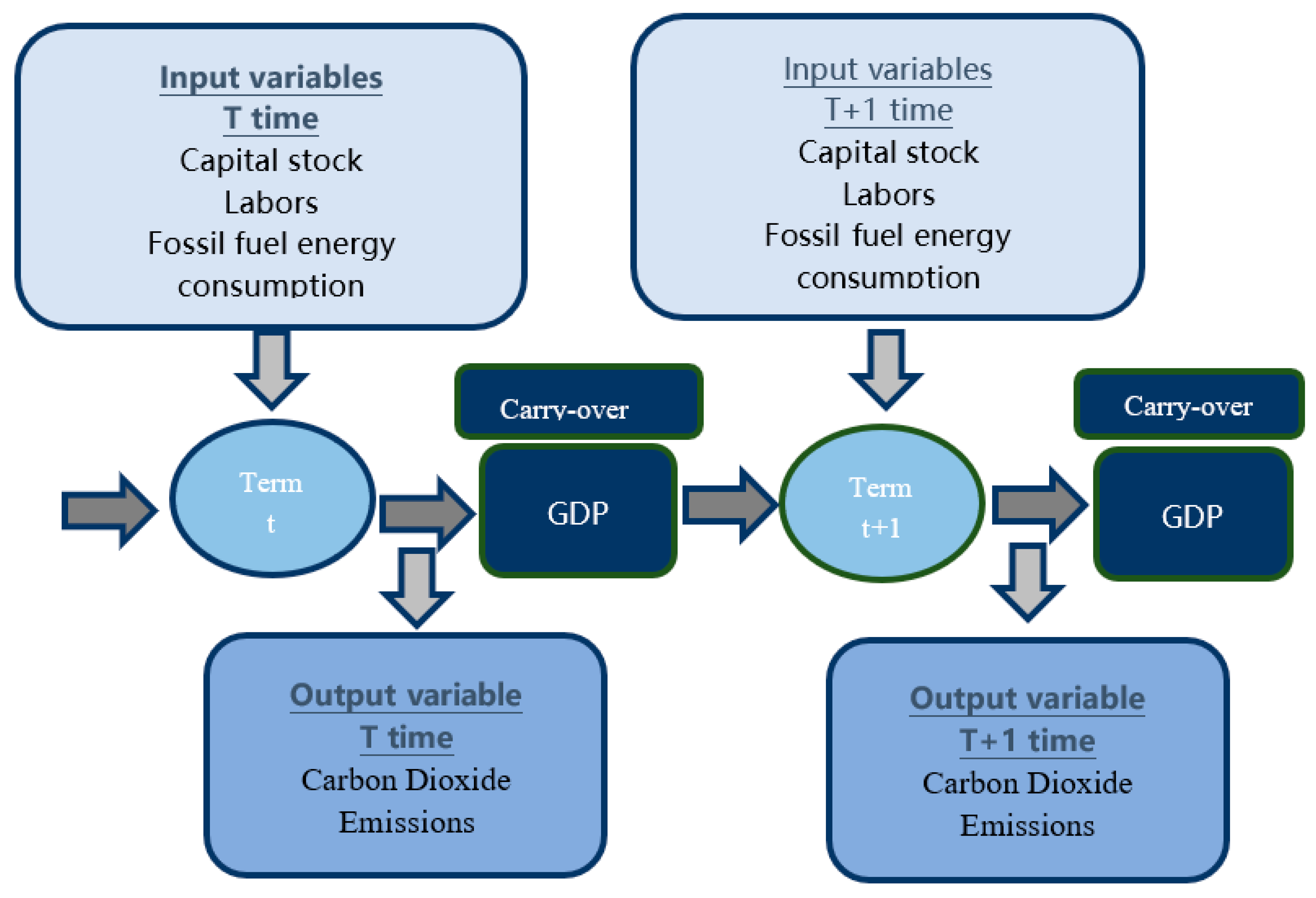
In this study, the energy efficiency rates of APEC economies are evaluated by dynamic DEA with nonoriented variable returns-to-scale models, which intend to estimate the energy efficiency values and analyze related policy implications of APEC economies, based on empirical results, and to expand the applicable measurements of all economies’ energy efficiency, based on this study, so that energy policies can be adjusted in a timely manner under the condition that all economies can pursue economic development and thus make the ecological environment of the earth sustainable. Therefore, this study collects the data of APEC economies to measure their energy efficiency over the period 2010–2014 and studies the impacts of undesirable outputs vs. energy efficiency ranking. We use labor force, actual capital stock, and energy consumption as the input variables in dynamic DEA models, while the undesirable output variable is CO₂ emissions, which is calculated by fossil fuel from 2010 to 2014. In the model, the carry-over variable is the real GDP. Dynamic DEA with nonoriented variable returns-to-scale models is utilized for related discussions.

This study is organized as follows: Section 2 presents the dynamic DEA model; Section 3 displays the estimated results of empirical measurement; Section 4 offers a discussion based on the results from the last section; Section 5 presents the conclusions and policy implications.

2. Materials and Methods

2.1. Performance Model

DEA is a method that applies several inputs to produce related outputs in a given time period to measure the relative efficiency of a set of decision-making units (DMUs). Various approaches can be used to measure efficiency changes during a certain period; for instance, window analysis and the Malmquist index [58]; Klopp [59] came up with window analysis, and the Malmquist Index was proposed by Färe et al. [11]. When considering the effect of the time change, these models usually ignore the carry-over activity between period t and period t + 1 and only focus on a single time period, aiming at local optimization. In the real business world, long-term planning and investment is a major problem for companies to improve business. The dynamic DEA model proposed by Färe and Grosskopf [6] is the first innovative contribution to solve this problem by introducing the dynamic aspects of production into the traditional DEA model in the case of multiple outputs. They framed several intertemporal methods, which laid a solid foundation for most later studies on dynamic DEA models. Later, Chen [60], Kao [61], Nemoto and Goto [62], Sueyoshhi and Sekitani [48], and Chang et al. [63] developed dynamic DEA, and Tone and Tsutsui [53] incorporated SBM into dynamic DEA.

The resulting model is nonoriented and can handle inputs and outputs separately, indicating that the model is suitable for nonuniformly distributed inputs and outputs, which can assign related weights according to their importance. Tone and Tsutsui divided carry-over variables into four categories, which serve as the analysis basis for the dynamic DEA models: (1) desirable, (2) undesirable, (3) free, and (4) fixed. The variables can be divided into three types: input, output, and nonoriented.

In addition, in terms of the features of carry-overs, this study views real GDP as the desirable carry-over variable, corresponding to the profits carried over from GDP to the next period. This research mainly concentrates on the idea that governments must promote economic growth without increasing CO₂ emissions. Thus, the performance of GDP in period t will exert an influence on the efficiency of period t + 1. The dynamic SBM model is used in this study to evaluate the overall efficiency of DMUs, as well as term efficiency; in these cases, the single-period optimization model is not suitable for performance evaluation. To consider the long-term perspective, the dynamic DEA model adds carry-over activities, which enables us to evaluate the specific efficiency of one period based on long-term optimization of the whole period. The estimated processes of the overall and term efficiencies under dynamic DEA model conditions are shown in Figure 1.

2.2. Samples and Data

In this study, a total of 21 APEC economics were taken as the original subjects; however, the data of “Papua New Guinea” were not completely collected; thus, the remaining 20 economies were taken as the subjects, and the study samples are shown in

Table 3. The summary of the APEC economies.

Economies	Join Time	Geography
Australia	November, 1989	Oceania
Brunei Darussalam	November, 1989	Asia
Canada	November, 1989	America
Indonesia	November, 1989	Asia
Japan	November, 1989	Asia
Malaysia	November, 1989	Asia
New Zealand	November, 1989	Oceania
South Korea	November, 1989	Asia
Singapore	November, 1989	Asia
Thailand	November, 1989	Asia
The Philippines	November, 1989	Asia
The United States	November, 1989	America
Chinese Taipei	November, 1991	Asia
Hong Kong, China	November, 1991	Asia
China	November, 1991	Asia
Mexico	November, 1993	America
Papua New Guinea	November, 1993	Oceania
Chile	November, 1994	America
Peru	November, 1998	America
Russia	November, 1998	Europe
Vietnam	November, 1998	Asia

Note: There is no database or official statistical yearbook to publish APEC’s Fossil fuel energy consumption after 2015. Additionally, the data from a certain country is not included in the Carbon dioxide emission data. Therefore, this study has compiled the latest public information of World Bank and UN data from 2010 to 2014 to analyze the implications of energy investment and the efficiency policies of APEC economies. Fossil fuel energy consumption: https://data.worldbank.org/indicator/EG.USE.COMM.FO.ZS (accessed on 29 June 2021). CO₂ emissions: https://data.worldbank.org/indicator/EN.ATM.CO2E.KT (accessed on 29 June 2021). Greenhouse Gas (GHGs) Emissions: http://data.un.org/Data.aspx?q=co2&d=GHG&f=seriesID%3aGHG (accessed on 29 June 2021). Carbon dioxide (CO₂) Emissions: http://data.un.org/Data.aspx?q=carbon+dioxide&d=GHG&f=seriesID%3aCO2 (accessed on 29 June 2021).

.

The basic discussion period of this paper is from 2010 to 2014, and the latest and most complete publicly quantifiable statistical data of the five consecutive years are used. (Due to the limitation of study time and difficulty in obtaining national quantitative data, and because some obtained statistical data are incomplete, the most complete and publicly external quantifiable data of the past five years were obtained for analysis.) The data sources come from (1) UN data, (2) The World Bank, and (3) Directorate General of Budget, Accounting and Statistics, Executive Yuan, Taiwan.

In this study, energy efficiency was evaluated by the dynamic DEA with nonoriented variable returns-to-scale models to estimate efficiency values according to the nonoriented method and to consider the differences between input items and output items, where the estimated efficiency values are all between 0 and 1. Under the given inputs, the maximum efficiency can be achieved; that is, the maximum output is obtained. The output result may be the expected desirable output, namely, good output; however, it may be accompanied by undesirable output, namely, bad output, which will decrease the overall efficiency value; therefore, the expected value of the variable shall be as small as possible.

This study selected 3 items, capital stock, labor, and fossil fuel energy consumption, as the inputs of the nonoriented variable returns-to-scale models of dynamic DEA. Carbon dioxide emissions are the undesirable output, and GDP is the intertemporal carry-over variable of desirable output. The definitions of the input, output, and intertemporal conversion variables in this study are collected and described, as shown in

Table 4. The definitions of inputs, outputs, and carry-over variables.

Variables		Definition	Trend
Inputs	Capital (Million Dollars)	The total amount of capital at a given point in an economy.	↓
	Labors	The population with the ability and willingness to work in or looking for work during the data standard week.	↓
	Fossil fuel energy consumption (Tons)	The energy use of natural resources, including coal, oil, and natural gas.	↓
Undesirable output	Carbon dioxide emission (million tons)	Average greenhouse gas emissions from the production, transportation, use, and recycling of the product.	↓
Desirable output Carry-over	GDP (Million Dollars)	The total value of all products and goods produced in an economy over a given period of time.	↑

.

According to the undesirable output model of Fare, Grosskopf, Lovell, and Pasurka [31], Seiford and Zhu [39] used DEA output-oriented BCC models as the basis to consider the problems of desirable outputs (good) and undesirable outputs (bad). The feature of DEA classification invariance was used to transform data adjustments and maintain linearity and geometric convexity. Seiford and Zhu [39] decomposed the outputs, as shown in the model below, where $Y^g$ is the desirable output, representing good output, $Y^b$ is the undesirable output, representing bad output, and the gross output is Y = $Y^g+Y^b$.

$$\left[\begin{array}{c}X\\ -X\end{array}\right]=\left[\begin{array}{c}{Y}^g\\ Y^b\\ -x\end{array}\right]$$

(1)

In traditional DEA models, it is assumed that a larger Y value ($Y^g+Y^b$) represents higher efficiency, where the increase in undesirable output $Y^b$ will reduce efficiency. All previous studies related to undesirable output values referred to the data translation adjustment mode of Seiford and Zhu [39] for processing; after the maximum value of an undesirable output is adjusted to a small value of 1 or 0.01, the values of all decision-making units are translated, and then, the efficiency performances of all DMUs are measured. Therefore, the suggested adjustment of the difference variables for undesirable outputs is less significant, and it is difficult to propose proper improvement suggestions through empirical analyses; thus, the suggested adjustment range of measuring efficiency and the difference variables of undesirable outputs is relatively limited. Hence, to improve the above limitation, in this study, translation adjustment was adopted for the value of an undesirable output $Y^b$, while in DMUs, the maximum value of $Y^b$ was adjusted to the minimum value, and the minimum value of $Y^b$ was adjusted to the maximum value. In this way, more appropriate suggestions were made for the adjustment range of the undesirable output values in this study, which had little effect on evaluating the efficiency values of all DMUs. This innovative adjustment mode provided an objective and reasonable description of undesirable output values and efficiency values, which is beneficial for this result analysis. Therefore, the undesirable output variable is adjusted as $\overline{Y_j^b}=W-Y_j^b+2min{Y}_j^b>0$, where $W=\left(\max Y_j^b-min{Y}_j^b\right)$.

2.3. Study of the Descriptive Statistics of Variables

In this study, descriptive statistical analysis was conducted on 20 APEC economies from 2010 to 2014 according to inputs, outputs, existence durations, and other relevant variable data of each year to understand the relationships among all variables. The descriptive statistical analyses of the input and output variable data of APEC economies from 2010 to 2014 are selected in this study, as shown in

Table 5. Descriptive statistics for variables of APEC economies during 2010–2014.

Variables		Mean	Max.	Min.	S.D.
2010
inputs	Capital	466,708.77	2,904,643.81	392.00	854,077.76
	Labors	74,499,482.70	778,967,720.00	189,509.00	170,866,513.70
	Fossil fuel energy consumption	2908.08	13,235.00	22.00	3134.33
Undesirable output	Carbon dioxide emissionsafter conversion	7,752,164.68	8,776,040.42	8203.08	2,181,022.79
Carry-over	GDP	1,814,811.67	14,964,372.00	13,707.37	3,535,616.53
2011
inputs	Capital	532,101.13	3,611,037.69	375.00	985,004.68
	Labors	75,094,431.80	784,390,231.00	192,391.00	171,999,803.80
	Fossil fuel energy consumption	2478.48	11,889.00	31.00	2834.58
Undesirable output	Carbon dioxide emissionsafter conversion	8,651,583.39	9,733,538.12	9695.55	2,351,256.45
Carry-over	GDP	2,018,737.71	15,517,926.00	18,525.32	3,757,267.94
2012
inputs	Capital	575,291.98	4,043,534.05	350.00	1,087,316.24
	Labors	75,746,834.50	789,130,421.00	194,864.00	173,015,145.44
	Fossil fuel energy consumption	4342.36	25,205.00	32.00	6506.39
Undesirable output	Carbon dioxide emissionsafter conversion	8,933,792.46	10,028,573.94	9666.21	2,394,092.72
Carry-over	GDP	2,129,974.08	16,155,255.00	19,048.50	3,954,016.76
2013
inputs	Capital	600,196.53	4,552,646.95	369.00	1,188,002.44
	Labors	76,244,213.70	793,347,524.00	197,026.00	173,914,054.72
	Fossil fuel energy consumption	1972.22	11,457.60	57.00	2531.17
Undesirable output	Carbon dioxide emissionsafter conversion	8,694,890.22	10,258,007.13	7803.38	3,027,696.82
Carry-over	GDP	2,176,995.27	16,691,517.00	18,093.83	4,095,094.13
2014
inputs	Capital stock	616,077.06	4,927,523.85	385.00	1,276,954.69
	Labors	76,757,707.10	796,905,370.00	199,025.00	174,674,523.98
	Fossil fuel energy consumption	1858.85	11,831.10	60.00	2611.35
Undesirable output	Carbon dioxide emissionsafter conversion	8,745,654.06	10,291,926.88	9108.83	3,057,603.14
Carry-over	GDP	2,233,312.89	17,393,103.00	17,123.13	4,299,553.87

.

2.4. Dynamic-SBM-ENERGY DEA Model

2.4.1. Production Possibility Set

This study considers n $DM{U}_k$ (k = 1, …, n) over time t (t = 1, …, T). Each DMU has common inputs (i = 1, 2, …, p; m = 1, 2, …, $n_{energy}$) and output (j = 1, 2, …, q). Consider $x_{ikt}\left(i=1,\dots ,p\right)$ and $y_{jkt}\left(j=1,\dots ,q\right),e_{mkt}\left(m=1,\dots ,n_{energy}\right)$ denotes the observed (discretionary) input and (discretionary) output values of $DM{U}_h$ at time t, respectively. We symbolize the category link as $z_{iht}^{good}$, which means desirable carry-over, such as GDP. We define the notion $z_{lht}^{good}forintended-output$ ($l$ = 1, …, $n^0{}_{bad}$; t = 1, …, T) to denote a good link value, where $n^0{}_{bad}$ is the number of good links. We define the notion $z_{mht}^{good}forinput$ ($l$ = 1, …, $n_{energy}$; t = 1, …, T) to denote a good link value, where $n_{energy}$ is the number of good links,

$$T=\left\{(X_{\mathit{iht}},y_{\mathit{jht}},e_{\mathit{mht}})|\begin{array}{c}{{\displaystyle \sum }}_{\begin{array}{c}k=1\\ k\ne h\end{array}}^n{\lambda }_k{}^t{X}_{\mathit{ikt}}\le X_{\mathit{iht}},i=1, 2,\dots ,p,t=1, 2, \dots ,T;{{\displaystyle \sum }}_{\begin{array}{c}k=1\\ k\ne h\end{array}}^n{\lambda }_k{}^t{e}_{\mathit{mkt}}\le e_{\mathit{mht}}\\ m=1, 2,\dots ,n_{\mathit{energy}},t=1, 2,\dots ,T\\ {{\displaystyle \sum }}_{\begin{array}{c}k=1\\ k\ne h\end{array}}^n{\lambda }_k{}^t{y}_{\mathit{jkt}}\ge y_{\mathit{jht}},j=1,2,\dots ,q,,t=1,2,\dots ,T;\\ {{\displaystyle \sum }}_{\begin{array}{c}k=1\\ k\ne h\end{array}}^n{\lambda }_k{}^t=1,{\lambda }_k{}^t\ge 0,\\ k=1,2,\dots ,n;j\ne h\\ {{\displaystyle \sum }}_{k=1}^n{z}_{\mathit{lkt}}^{\mathit{good}}\ast {\lambda }_k^t\ge z_{\mathit{lkt}}^{\mathit{good}},\\ l=1,2,\dots ,n,t=1,2,\dots ,T;\end{array}\right\}$$

(2)

This constraint is very important for the Dynamic SBM Energy DEA model, as it connects the activities between time t and t + 1.

2.4.2. Dynamic-SBM-ENERGY Model

We express $DM{U}_k\left(k=1,\dots ,n\right)$ under the above production possibility sets and define nonoriented efficiency under the goal of maximizing output and minimizing input, as shown in the following:

Model:

• let the set of DMUs be k = 1, 2, 3, …, n, over T terms (t = 1, 2, 3,…, T);
• the input of x be i = 1, 2, 3, …, p;
• the energy input of x be m = 1, 2, 3, …, $n_{energy}$;
• $the output of y be j=$1, 2, 3, …, q;
• z = carry over with good categories, i.e., The carry-over of this article is GDP;
• $l=1, 2,\dots , n^0{}_{bad}$; m = 1, 2, 3, …, $n_{energy}$;
• W = weight: $W^t for time period$, $W^i for$ input, and $W^j for$ output.

The following is the nonoriented Model:

$${\alpha }_0{}^{\ast } =min\frac{{{\displaystyle \sum }}_{t=1}^T{W}^t[1-\frac{1}{p+n_{\mathit{energy}}}({{\displaystyle \sum }}_{i=1}^p\frac{w^i\ast s_{\mathit{it}}^{-}}{x_{\mathit{iht}}}+{{\displaystyle \sum }}_{m=1}^{n_{\mathit{energy}}}\frac{s_{\mathit{mt}}^{-}{}^{\mathit{energy}}}{z_{\mathit{mht}}^{\mathit{good}}})]}{{{\displaystyle \sum }}_{t=1}^T{W}^t[1+\frac{1}{q+n^o{}_{\mathit{bad}}}({{\displaystyle \sum }}_{j=1}^q\frac{w^j\ast s_{\mathit{jt}}^{+}}{y_{\mathit{jht}}}+{{\displaystyle \sum }}_{l=1}^{n^o{}_{\mathit{bad}}}\frac{s_{\mathit{lt}}^{+}{}^{\mathit{bad}}}{z_{\mathit{lht}}^{\mathit{good}}})]}$$

(3)

$${{\displaystyle \sum }}_{k=1}^n{z}_{\mathit{lkt}}{}^{\ast }{\lambda }_k^t={{\displaystyle \sum }}_{k=1}^n{z}_{\mathit{lkt}}{}^{\ast }{\lambda }_k^{t+1},\forall l,t=1, 2,\dots ,T+1,$$

(3a)

$$\begin{gathered} S.t. \\ {x}_{\mathit{iht}}={{\displaystyle \sum }}_{k=1}^n{x}_{\mathit{ikt}}{}^{\ast }{\lambda }_k^t+s_{\mathit{it}}^{-},i=1,\dots ,t=1,3,T \end{gathered}$$

(4)

$$e_{mht}={{\displaystyle \sum }}_{k=1}^n{e}_{mkt}{}^{\ast }{\lambda }_k^t+s_{ft}^{-energy},m=1,2,\dots , n_{energy},t=1,2,3,\dots ,T$$

(5)

$$y_{jht}={{\displaystyle \sum }}_{k=1}^n{y}_{jkt}{}^{\ast }{\lambda }_k^t-s_{jt}^{+},j=1,2,\dots ,q,t=1,2,3,\dots ,T$$

(6)

$$z_{lht}^{good}={{\displaystyle \sum }}_{k=1}^n{z}_{lht}^{good}{}^{\ast }{\lambda }_k^t-s_{lt}^{+}{}^{good},l=1,2,\dots , n^0{}_{bad},t=1,2,3,\dots ,T$$

(7)

where output $z_{lht}^{good}$ is carry-over for good category

$$z_{\mathit{mht}}^{\mathit{good}}={{\displaystyle \sum }}_{k=1}^n{z}_{\mathit{mht}}^{\mathit{good}}{}^{\ast }{\lambda }_k^t-s_{\mathit{mt}}^{+\mathit{energy}},m=1,2,\dots ,n_{\mathit{energy}},t=1,2,3,\dots ,T$$

(8)

where input $z_{mht}^{good}$ is carry-over for good category

$${{\displaystyle \sum }}_{k=1}^n{\lambda }_k^t=1,\left(\mathit{\text{VRS-setting}}\right)$$

(9)

$${\lambda }_k^t\ge 0,s_{\mathit{it}}^{-}\ge 0,s_{\mathit{lt}}^{+\mathit{bad}}\ge 0,s_{\mathit{mt}}^{-\mathit{energy}}\ge 0,s_{\mathit{jt}}^{+}\ge 0\forall i,j,m,l,t$$

(9a)

where

• $s_{it}^{-}:$ slacks of good input;
• $s_{jt}^{+}:$ slacks of good output;
• $s_{mt}^{-energy}$: slacks of energy input;
• $s_{lt}^{+bad}$: slacks of bad output (i.e., Carbon dioxide emissions) after conversion.

Here is the solution with the most efficiency:

$${\alpha }_{0t} =\frac{[1-\frac{1}{p+n_{\mathit{energy}}}\left({{\displaystyle \sum }}_{i=1}^p\frac{W^i{\ast s}_{\mathit{it}}^{-}}{x_{\mathit{iht}}}+{{\displaystyle \sum }}_{m=1}^{n_{\mathit{energy}}}\frac{s_{\mathit{mt}}^{-\mathit{energy}}}{z_{\mathit{mht}}^{\mathit{good}}})\right]}{[1+\frac{1}{q+n^o{}_{\mathit{bad}}}({{\displaystyle \sum }}_{j=1}^q\frac{w^j{\ast s}_{\mathit{jt}}^{+}}{y_{\mathit{jht}}}+{{\displaystyle \sum }}_{l=1}^{n^o{}_{\mathit{bad}}}\frac{s_{\mathit{lt}}^{+}{}^{\mathit{bad}}}{z_{\mathit{lht}}^{\mathit{good}}})]}$$

(10)

where $s_{it}^{-},s_{jt}^{+},s_{lt}^{+bad},s_{mt}^{-energy}$ are slacks denoting input excess, output shortfall, intended-output shortfall, and energy -input excess, respectively. The $w_i^{+}$ is the weight to output i and must fit the following condition: ${{\displaystyle \sum }}_{i=1}^p{W}^i=p$. Similarly, the $w_i^{-}$ is the weight of input I and satisfies the condition: ${{\displaystyle \sum }}_{j=1}^q{w}^j=q$. The $w^t$ is the weight to time t and satisfies the condition: ${{\displaystyle \sum }}_{t=1}^T{w}^t=T$.

3. Empirical Results and Analysis

In this study, the nonoriented variable returns-to-scale of dynamic DEA was employed to measure the energy efficiency of 20 APEC economies from 2010 to 2014, determine the relatively inefficient parts, and make suggestions for improvement directions, as well as the ranges of different variables, to explore changes in the intertemporal conversion variables of APEC economies and make improvement suggestions.

3.1. Energy Efficiency Analysis

The study employs the nonoriented variable returns-to-scale dynamic DEA model to measure the annual and overall energy efficiency of 20 APEC economies from 2010 to 2014. The results are analyzed and collected in

Table 6. The energy efficiency of APEC economies from 2010 to 2014.

Economies	2010	2011	2012	2013	2014	Overall	Ranking
Taiwan	1.0000	1.0000	0.4840	0.4867	0.4501	0.6905	8
Australia	1.0000	1.0000	1.0000	1.0000	1.0000	1.0000	1
Brunei	1.0000	1.0000	1.0000	1.0000	1.0000	1.0000	1
Canada	0.6846	0.7551	0.7413	0.7064	0.6609	0.7097	7
Chile	0.4374	0.4199	0.4115	0.4415	0.5111	0.4442	10
China	0.0009	0.0008	0.0009	0.0005	0.0005	0.0007	20
Hong Kong	0.9652	0.9109	0.6132	0.1079	0.9609	0.4258	11
Indonesia	0.3361	0.2972	0.1878	0.2563	0.2882	0.2737	18
Japan	0.9998	0.9997	1.0000	1.0000	0.9987	0.9996	5
South Korea	0.3990	0.3968	0.4414	0.4310	0.4216	0.4179	13
Mexico	0.4783	0.4859	0.4994	0.4962	0.0954	0.2622	19
Malaysia	0.3699	0.4452	0.3946	0.4366	0.4801	0.4250	12
The New Zealand	1.0000	1.0000	1.0000	1.0000	1.0000	1.0000	1
Peru	0.3841	0.3859	0.3679	0.3869	0.4670	0.3981	15
The Philippines	0.3779	0.3938	0.4528	0.4200	0.4082	0.4101	14
Russia	0.3866	0.4362	0.4952	0.4575	1.0000	0.5445	9
Singapore	1.0000	1.0000	1.0000	0.9701	0.9656	0.9871	6
Thailand	0.3056	0.2957	0.2938	0.3187	0.3805	0.3189	16
The United States	1.0000	1.0000	1.0000	1.0000	1.0000	1.0000	1
Vietnam	0.2294	0.2822	0.3124	0.3797	0.3966	0.3176	17
Mean	0.6177	0.6253	0.5848	0.5648	0.6268	0.5813	-
Max	1.0000	1.0000	1.0000	1.0000	1.0000	1.0000	-
Min	0.0009	0.0008	0.0009	0.0005	0.0005	0.0007	-
S.D.	0.3389	0.3323	0.3157	0.3223	0.3349	0.3162	-

.

From 2010 to 2014, the average overall energy efficiency was 0.5813, the maximum value was 1.000, the minimum value was 0.0007, and the standard deviation was 0.3162. The average energy efficiency rankings of eight economies, Taiwan, Australia, Brunei, Canada, Japan, New Zealand, Singapore, and the United States, were higher than the average overall energy efficiency ranking, while the average energy efficiency rankings of 12 economies, Chile, China, Hong Kong, Indonesia, Korea, Mexico, Malaysia, Peru, the Philippines, Russia, Thailand, and Vietnam, were lower than the average overall energy efficiency ranking. From 2010 to 2014, the APEC economies of the four economies with the best overall energy efficiency were Australia, Brunei, New Zealand, and the United States, meaning that all of their annual energy efficiencies were 1.0000 during the study period. Those with excellent performance can be regarded as the models from which other economies can learn. The overall ranking was Japan, Singapore, Canada, Taiwan, Russia, Chile, Hong Kong, Malaysia, Korea, the Philippines, Peru, Thailand, and Vietnam. The top three economies with the worst overall energy efficiency ratings were Indonesia (0.2737), Mexico (0.2622), and China (0.0007), meaning there was much room for efficiency improvement. This is where the main findings of this paper differ from other literature. Regarding the energy use efficiency of China, the results of this paper are quite different from other results. China uses a large amount of energy and thus emits a large amount of carbon dioxide. Lu et al., 2019 concluded that China uses energy efficiently, but they failed to adjust the CO₂ data. In the future, the largest output of CO₂ will become the benchmark and then overmeasure the energy use efficiency of China.

Taiwan had the best energy efficiency levels in 2010 and 2011; however, its efficiency dropped in the last three years. While Vietnam has improved its energy efficiency level each year, its efficiency level is still less than 0.4. While Indonesia experienced a decrease in the first three years, its overall efficiency still shows a decreasing trend.

3.2. Improvement of the Input Items

The suggestions for improvement, as well as the ranges of different variables as inputs for APEC economies from 2010 to 2014, as selected by this study, are shown in

Table 7. The adjustment of input items for AEPC economies from 2010 to 2014.

Economies	Adjustment Range of Capital Stock (%)						Adjustment Range of Labor (%)						Adjustment Range of Consumption of Fossil Fuel Energy (%)
	2010	2011	2012	2013	2014	Mean	2010	2011	2012	2013	2014	Mean	2010	2011	2012	2013	2014	Mean
Taiwan	0.00	0.00	−100.00	−100.00	−100.00	−60.00	0.00	0.00	−56.95	−56.78	−56.55	−34.06	0.00	0.00	−91.97	−91.10	−91.18	−54.85
Australia	0.00	0.00	0.00	0.00	0.00	0.00	0.00	0.00	0.00	0.00	0.00	0.00	0.00	0.00	0.00	0.00	0.00	0.00
Brunei	0.00	0.00	0.00	0.00	0.00	0.00	0.00	0.00	0.00	0.00	0.00	0.00	0.00	0.00	0.00	0.00	0.00	0.00
Canada	−19.90	−8.15	−17.79	−14.64	−9.25	−13.95	−5.52	−8.97	−1.49	−4.42	−10.14	−6.11	−69.21	−56.36	−56.82	−69.03	−82.34	−66.75
Chile	−11.14	−18.57	−22.94	−15.66	0.00	−13.66	−59.55	−60.54	−60.85	−60.91	−60.22	−60.41	−94.30	−93.93	−92.63	−90.82	−86.19	−91.57
China	−45.48	−54.11	−55.49	−58.26	−59.29	−54.53	−88.35	−88.43	−88.40	−88.43	−88.42	−88.41	−68.76	−69.39	−58.30	−87.84	−90.03	−74.86
Hong Kong	−1.26	0.00	0.00	−10.39	0.00	−2.33	−0.95	−3.83	−19.79	−15.91	−2.38	−8.57	−8.24	−21.35	−96.24	−95.77	−9.35	−46.19
Indonesia	−36.37	−42.74	−73.57	−37.28	−33.40	−44.67	−91.77	−91.87	−87.28	−92.05	−92.09	−91.01	−64.07	−74.64	−81.97	−90.96	−86.42	−79.61
Japan	−0.01	−0.01	0.00	0.00	−0.01	−0.01	−0.01	−0.01	0.00	0.00	−0.10	−0.02	−0.05	−0.06	0.00	0.00	−0.27	−0.08
South Korea	−39.10	−42.83	−35.21	−31.03	−32.84	−36.20	−48.93	−49.64	−50.06	−50.45	−50.55	−49.93	−88.10	−87.01	−79.09	−87.79	−87.53	−85.90
Mexico	−10.57	−15.54	−12.74	−6.82	−3.82	−9.90	−75.59	−75.76	−76.56	−76.77	−77.13	−76.36	−65.32	−62.05	−57.73	−66.24	−59.98	−62.26
Malaysia	−71.48	−14.55	−21.46	−16.34	−11.26	−27.02	−49.86	−70.74	−71.84	−72.94	−73.29	−67.73	−62.77	−79.40	−87.47	−76.66	−69.09	−75.08
The New Zealand	0.00	0.00	0.00	0.00	0.00	0.00	0.00	0.00	0.00	0.00	0.00	0.00	0.00	0.00	0.00	0.00	0.00	0.00
Peru	−8.02	−10.10	−15.52	−11.84	−1.41	−9.38	−83.91	−83.95	−84.19	−84.06	−84.15	−84.05	−87.10	−85.90	−89.83	−86.12	−74.05	−84.60
The Philippines	0.00	0.00	0.00	0.00	0.00	0.00	−91.93	−92.01	−91.57	−92.09	−89.77	−91.47	−88.64	−84.20	−71.01	−81.68	−87.51	−82.61
Russia	−21.28	−21.82	−10.39	−2.55	0.00	−11.21	−71.70	−71.80	−71.55	−71.22	0.00	−57.25	−65.25	−65.04	−58.98	−79.94	0.00	−53.84
Singapore	0.00	0.00	0.00	−2.09	−2.23	−0.86	0.00	0.00	0.00	0.00	0.00	0.00	0.00	0.00	0.00	−6.89	−8.08	−2.99
Thailand	−22.08	−25.44	−28.26	−24.28	−4.27	−20.87	−88.57	−88.73	−88.68	−88.47	−88.40	−88.57	−95.09	−94.92	−93.91	−90.71	−90.79	−93.08
The United States	0.00	0.00	0.00	0.00	0.00	0.00	0.00	0.00	0.00	0.00	0.00	0.00	0.00	0.00	0.00	0.00	0.00	0.00
Vietnam	−28.86	−14.59	−13.16	−8.06	−9.28	−14.79	−95.41	−95.44	−95.51	−95.53	−95.52	−95.48	−97.38	−94.49	−90.96	−75.43	−74.68	−86.59
mean	−15.78	−13.42	−20.33	−16.96	−13.35	−15.97	−42.60	−44.09	−47.24	−47.50	−43.44	−44.97	−47.71	−48.44	−55.35	−58.85	−49.87	−52.04

. From 2010 to 2014, the average adjustment range of the capital stock was −15.97%, and the adjustment ranges of the capital stocks of five economies, Australia, Brunei, New Zealand, the Philippines, and the United States, were 0.00%, representing no need for adjustment. In contrast, the average suggested adjustment ranges of six economies, Taiwan, China, Indonesia, Korea, Malaysia, and Thailand, were higher than the overall average; these economies saw improvements in their usage of capital, especially Taiwan and China. This study finds that the adjustment ranges of the capital stocks of Russia and Vietnam show a gradual downward trend; in particular, the adjustment range of the capital stock of Russia was reduced to 0 in 2014, as it engaged in efficient capital usage. Canada, Mexico, Malaysia, and Peru show a downward trend of capital stocks.

The overall average adjustment range of labor was −44.97%, and the average suggested adjustment ranges of 11 economies, Chile, China, Indonesia, Korea, Mexico, Malaysia, Peru, the Philippines, Russia, Thailand, and Vietnam, were higher than the overall average, indicating that there is much room for improvement in the use of labor in these economies, particularly the Philippines and Indonesia. Furthermore, the adjustment ranges of China, Thailand, and Vietnam in terms of labor remained at an average level (88.41; 88.57; 95.48). The adjustment range of labor of three economies, Korea, Mexico, and Malaysia, showed a slight upward trend from 2010 to 2014.

Regarding the consumption of fossil fuel energy, the average adjustment range of the overall APEC economies was −52.04%. The adjustment range between 2010 and 2014 shows a fluctuation of rising, followed by falling. The average suggested adjustment ranges of 13 economies, Taiwan, Canada, Chile, China, Indonesia, Korea, Mexico, Malaysia, Peru, the Philippines, Russia, Thailand, and Vietnam, were higher than the overall average.

Based on the above information, four economies, Australia, Brunei, New Zealand, and the United States, had the best overall performance, and no adjustment was required for their input variables during the study period. Five economies, China, Indonesia, Korea, Malaysia, and Thailand, had the worst overall performance, meaning that their input variables during the study period were in the most urgent need of improvement, and the average suggested improvement range was higher than the overall average.

3.3. Improvement of Undesirable Outputs

The adjustment results of outputs are mainly summarized in

Table 8. The adjustment of undesirable output for APEC economies between 2010 and 2014.

Economies	Undesirable Output–Adjustment Range of Carbon Dioxide Emissions (%)
	2010	2011	2012	2013	2014	Mean
Taiwan	0.00	0.00	−1.26	−1.28	−1.32	−0.77
Australia	0.00	0.00	0.00	0.00	0.00	0.00
Brunei	0.00	0.00	0.00	0.00	0.00	0.00
Canada	0.00	0.00	0.00	0.00	0.00	0.00
Chile	−0.12	−0.19	−0.18	−0.24	−0.17	−0.18
China	−69,285.47	−69,120.30	−73,375.75	−93,545.64	−79,909.74	−77,047.38
Hong Kong	0.00	0.00	0.00	−900.26	0.00	−180.05
Indonesia	−1.72	−3.55	−2.73	−2.23	−1.90	−2.43
Japan	0.00	0.00	0.00	0.00	0.00	0.00
South Korea	−2.10	−2.22	−2.19	−2.20	−2.06	−2.15
Mexico	0.99	−1.19	−1.37	−1.25	−910.72	−183.10
Malaysia	−1.10	−1.51	−1.44	−1.59	−1.62	−1.45
The New Zealand	0.00	0.00	0.00	0.00	0.00	0.00
Peru	−0.24	−0.14	−0.16	−0.18	−0.22	−0.19
The Philippines	−0.28	−0.26	−0.25	−0.35	−0.22	−0.27
Russia	−13.63	−13.49	−14.17	−13.16	0.00	−10.89
Singapore	0.00	0.00	0.00	0.00	0.00	0.00
Thailand	−2.07	−1.84	−1.97	−1.96	−2.09	−1.99
The United States	0.00	0.00	0.00	0.00	0.00	0.00
Vietnam	−1.28	−1.26	−1.09	−1.12	−1.30	−1.21
mean	−3465.45	−3457.30	−3670.13	4723.57	−4041.57	−3871.60

and

Table 9. The adjustment of the intertemporal conversion variable GDP for APEC economies from 2010 to 2014.

Economies	Desirable Output—Adjustment Range of GDP (%)
	2010	2011	2012	2013	2014	Mean
Taiwan	0.00	0.00	6.83	7.08	8.01	4.38
Australia	0.00	0.00	0.00	0.00	0.00	0.00
Brunei	0.00	0.00	0.00	0.00	0.00	0.00
Canada	0.00	0.00	1.35	0.00	5.47	1.36
Chile	5.66	1.41	0.00	0.00	14.32	4.28
China	41.01	17.90	8.58	0.00	0.00	13.50
Hong Kong	0.00	1.14	0.00	0.00	0.00	0.23
Indonesia	12.04	0.00	0.25	5.07	12.39	5.95
Japan	0.00	0.00	0.00	0.00	0.03	0.01
South Korea	4.88	0.27	2.71	0.00	0.00	1.57
Mexico	6.04	0.00	2.82	0.51	1.96	2.27
Malaysia	7.75	1.11	0.00	3.10	3.36	3.06
The New Zealand	0.00	0.00	0.00	0.00	0.00	0.00
Peru	9.70	7.28	0.00	3.13	8.63	5.75
The Philippines	10.40	9.34	2.06	0.00	0.00	4.36
Russia	30.87	2.56	0.00	0.00	0.00	6.69
Singapore	0.00	0.00	0.00	0.00	0.00	0.00
Thailand	3.52	3.13	0.34	0.00	8.32	3.06
The United States	0.00	0.00	0.00	0.00	0.00	0.00
Vietnam	26.44	24.29	13.07	11.27	7.79	16.57
mean	7.92	3.42	1.90	1.51	3.51	3.65

. Based on the energy efficiency evaluation of 20 APEC economies, the analysis results in Table 8 show that the overall average adjustment range of carbon dioxide emissions of undesirable output variables for APEC economies from 2010 to 2014 was −3871.60%, and only China’s average suggested adjustment range was higher than the overall average. According to the definition of Seiford and Zhu (2002), regarding the adjustment mode of undesirable outputs, the high carbon dioxide emissions of China will cause underestimation of its energy use efficiency during evaluation, as high emissions will move China closer to the frontier in terms of possible production and even become the benchmark. Therefore, another translation adjustment mode of carbon dioxide emission is provided in this paper to measure the actual energy use efficiency of all economies to calculate whether they can actually be controlled or adjusted.

Based on the above information, the seven economies of Australia, Brunei, Canada, Japan, New Zealand, Singapore, and the United States had the best overall performance, and no adjustment was needed for their undesirable output variables during the study period. China was the country with the worst overall performance, its undesirable output variables during the study period were in the most urgent need of improvement, and the average suggested improvement range was higher than the overall average.

3.4. Changes in Intertemporal Conversion Variables and Improvement Suggestions

In this study, gross domestic product (GDP) was selected as the carry-over to link the current period and the next period to facilitate a more complete analysis of the effects of gross domestic product for overall energy efficiency evaluation. Moreover, an adjustment rate was proposed for intertemporal conversion variables, which would help APEC economies achieve a relatively efficient reference and facilitate desirable outputs (good results) being brought into the next period.

In this study, changes in intertemporal conversion variables and suggestions for the improvement of APEC economies from 2010 to 2014 were selected. The analysis results in Table 9 show that the overall average adjustment range of the gross domestic product of desirable output variables for APEC economies from 2010 to 2014 was 3.65%, and the average suggested adjustment range of eight economies, Taiwan, Chile, China, Indonesia, Peru, the Philippines, Russia, and Vietnam, was higher than the overall average. Based on the above information, five economies, Australia, Brunei, New Zealand, Singapore, and the United States, had the best overall performance, and no adjustment was needed for their desirable output variables during the study period. Eight economies, Taiwan, Chile, China, Indonesia, Peru, the Philippines, Russia, and Vietnam, have the worst overall performance, and their intertemporal conversion variables are in the most urgent need of improvement. Furthermore, while China and Vietnam have the largest adjustments at 13.5% and 16.57%, respectively, their adjustments show a declining trend year by year, particularly China, where the adjustment range of the GDP was reduced to 0 in 2013. In other words, when considering the economic growth of the previous period, China’s adjustment to GDP output is optimal.

4. Energy Policy Implications of APEC Economies

The variables selected in this study were used to analyze the energy inputs and policy improvement directions of all economies, as well as efficiency policy implications, to achieve the optimal efficiency targets. While reducing capital stock, labor, fossil fuel energy consumption, and carbon dioxide emissions and increasing gross domestic production can increase energy efficiency, economies do not want to reduce the state’s capital stock; because labor is related to population birth, adjustments are difficult; thus, adjustments can only start from fossil fuel energy consumption, carbon dioxide emissions, and gross domestic production. Hence, this study analyzes the effects of adjustments to fossil fuel energy consumption and carbon dioxide emissions on gross domestic production to analyze the implications of efficiency policies.

As shown in

Table 10. A summary of energy efficiency, ranking, and adjustment arrangement of variables for APEC economies.

Economies	Efficiency	Ranking	Capital Stock	Labors	Fossil Fuel Energy Consumption	Carbon Dioxide Emissions	GDP	Developed/ Developing
			Average Adjustment Range (%)
Taiwan	0.6905	8	−60.00	−34.06	−54.85	−0.77	4.38	Developed
Australia	1.0000	1	0.00	0.00	0.00	0.00	0.00	Developed
Brunei	1.0000	1	0.00	0.00	0.00	0.00	0.00	Developing
Canada	0.7097	7	−13.95	−6.11	−66.75	0.00	1.36	Developed
Chile	0.4442	10	−13.66	−60.41	−91.57	−0.18	4.28	Developing
China	0.0007	20	−54.53	−88.41	−74.86	−77,047.38	13.50	Developing
Hong Kong	0.4258	11	−2.33	−8.57	−46.19	−180.05	0.23	Developed
Indonesia	0.2737	18	−44.67	−91.01	−79.61	−2.43	5.95	Developing
Japan	0.9996	5	−0.01	−0.02	−0.08	0.00	0.01	Developed
South Korea	0.4179	13	−36.20	−49.93	−85.90	−2.15	1.57	Developed
Mexico	0.2622	19	−9.90	−76.36	−62.26	−183.10	2.27	Developing
Malaysia	0.4250	12	−27.02	−67.73	−75.08	−1.45	3.06	Developing
New Zealand	1.0000	1	0.00	0.00	0.00	0.00	0.00	Developed
Peru	0.3981	15	−9.38	−84.05	−84.60	−0.19	5.75	Developing
The Philippines	0.4101	14	0.00	−91.47	−82.61	−0.27	4.36	Developing
Russia	0.5445	9	−11.21	−57.25	−53.84	−10.89	6.69	Developing
Singapore	0.9871	6	−0.86	0.00	−2.99	0.00	0.00	Developed
Thailand	0.3189	16	−20.87	−88.57	−93.08	−1.99	3.06	Developing
The United States	1.0000	1	0.00	0.00	0.00	0.00	0.00	Developed
Vietnam	0.3176	17	−14.79	−95.48	−86.59	−1.21	16.57	Developing
mean	0.5813	-	−15.97	−44.97	−52.04	−3871.60	3.65	-

, the average overall energy efficiency of APEC economies from 2010 to 2014 was 0.5813. The overall energy efficiency of eight economies, Australia, Brunei, New Zealand, the United States, Japan, Singapore, Canada, and Taiwan, was higher than the average overall energy efficiency of APEC economies, and, except for Brunei, those above eight are developed economies. (Developed country: also known as an advanced country. It refers to a country with high levels of economic and social development, as well as high living standards, also known as a more economically developed country (MEDC). The general characteristics of a developed country are a high human development index, per-capita gross national product, industrialization level, and life quality.) The overall energy efficiency ratings of 12 economies, Russia, Chile, Hong Kong, Malaysia, Korea, the Philippines, Peru, Thailand, Vietnam, Indonesia, Mexico, and China, were lower than the average overall energy efficiency of APEC economies, and, except for Hong Kong and Korea, the above 12 economies were developing economies. (Developing country: also known as a less developed country. It refers to a country with lower levels of economic and social development than a developed country. With the development of the economy, the difference in living standards between some developing countries and developed countries is not large.) To pursue national competitiveness and improve their international status, developing economies excessively input fossil fuel energy while actively increasing their gross domestic product, which increases excessive carbon dioxide emissions and leads to low national energy efficiency. Based on the empirical results, the inputs of fossil fuel energy can improve the gross domestic product and carbon dioxide emissions with changes in the same direction, while inputs of fossil fuel energy and outputs of carbon dioxide emissions can reduce energy efficiency with changes in the opposite direction.

In conclusion, it is difficult to reduce fossil fuel energy consumption and carbon dioxide emissions while simultaneously raising gross domestic production. In pursuit of economic growth, it is difficult for economies to increase their desirable output—gross domestic product while reducing undesirable outputs—carbon dioxide emissions. These study results are the same as those proposed by Chiu et al., 2017; economies must enact cuts in policy and technical areas, appropriately adjust their energy policies, and actively develop new energy technologies, such as collecting carbon taxes, replacing fossil fuel energy with renewable energy, developing clear alternative energy programs, and establishing diversified energy structures, to effectively reduce carbon dioxide emissions and achieve optimal energy efficiency.

5. Conclusions and Suggestions

For global warming, governments of all economies have begun to consider environmental factors while pursuing economic growth. In this study, the effects of undesirable output variables and carry-over variables are measured to rank 20 APEC economies. The results indicate that, from 2010 to 2014, the APEC economies with overall energy efficiency included for economies, Australia, Brunei, New Zealand, and the United States, and all their annual energy efficiencies were 1.0000 during the study period. Those with excellent performance can be regarded as models from which other economies can learn.

To improve energy efficiency, economies are expected to enact cuts through policy and technical approaches, more specifically, through appropriately adjusting their energy policies and actively developing new energy technologies. Good energy efficiency policies are helpful to improve energy efficiency targets. Hence, discussions by APEC economies regarding energy efficiency can provide positive directions for economies to set their energy efficiency targets to offer references for future targets, directions, and policy adjustments to achieve energy savings and carbon emission reduction. Since China has a poor performance of energy efficiency, it can introduce advanced technologies from developed APEC economies, as well as developing green finance towards the target of sustainable development.

Relevant suggestions can be made as follows:

• Based on the results of this study, it is difficult to reduce fossil fuel energy consumption and carbon dioxide emissions while simultaneously raising gross domestic production to improve energy efficiency; thus, all counties are suggested to actively develop alternative energy technologies and improve their efficiency ratings to reduce dependence on fossil fuel energy and carbon dioxide emissions and improve their energy efficiency. To further confirm the correctness of the study results, the energy data of different global economies can be further searched and collected as a follow-up extension of this study, which will render the results more convincing.
• This study period was from 2010 to 2014; in 2015, economies submitted their Intended Nationally Determined Contributions to the United Nations Framework Convention on Climate Change, which indicated their future carbon reduction goals and strategies. It is suggested that future researchers continue from 2015 to analyze whether the economies reduced their carbon emissions and achieved their anticipated goals according to their Intended Nationally Determined Contributions and then analyze whether the energy efficiency ratings of such economies were improved.
• In this study, the nonoriented variable returns-to-scale model of the dynamic DEA was selected to analyze the energy efficiency ratings of APEC economies, and APEC economies may make appropriate adjustments and amendments to their energy policies based on the results when formulating policies related to energy in the future. Regarding studies of energy efficiency, future researchers should consider other measurement methods or add time series analysis of longitudinal sections and incorporate other factors, such as alternative energy use, per capita land-use area, and per capita income of each country, to further discuss and analyze energy efficiency.

References

1. Pittman, R.W. Issues in pollution control: Interplant cost differences and economies of scale. Land Econ. 1981, 57, 1–17. [Google Scholar] [CrossRef]
2. Weber, W.L.; Bruce, D. Productivity growth and pollution in state manufacturing. Rev. Econ. Stat. 2001, 83, 195–199. [Google Scholar] [CrossRef]
3. Zofio, J.L.; Prieto, A.M. Environmental efficiency and regulatory standards: The case of CO2 emissions from OECD industries. Resour. Energy Econ. 2001, 23, 63–83. [Google Scholar] [CrossRef]
4. Zhou, P.; Ang, B.W.; Poh, K.L. Slacks-based efficiency measures for modeling environmental performance. Ecol. Econ. 2006, 60, 111–118. [Google Scholar] [CrossRef]
5. Zhou, P.; Poh, K.L.; Ang, B.W. A non-radial DEA approach to measuring environmental performance. Eur. J. Oper. Res. 2007, 178, 1–9. [Google Scholar] [CrossRef]
6. Färe, R.; Grosskopf, S. Intertemporal production frontiers: With dynamic DEA. J. Oper. Res. Soc. 1997, 48, 656. [Google Scholar] [CrossRef]
7. Wang, C. Decomposing energy productivity change: A distance function approach. Energy 2007, 32, 1326–1333. [Google Scholar] [CrossRef]
8. Zaim, O. Measuring environmental performance of state manufacturing through changes in pollution intensities: A DEA framework. Ecol. Econ. 2004, 48, 37–47. [Google Scholar] [CrossRef] [Green Version]
9. Pasurka, C.A., Jr. Decomposing electric power plant emissions within a joint production framework. Energy Econ. 2006, 28, 26–43. [Google Scholar] [CrossRef]
10. Zhou, P.; Ang, B.W. Decomposition of aggregate CO2 emissions: A production theoretical approach. Energy Econ. 2008, 30, 1054–1067. [Google Scholar] [CrossRef]
11. Färe, R.; Grosskopf, S.; Norris, M.; Zhang, Z. Productivity growth, technical progress and efficiency change in industrialized countries. Am. Econ. Rev. 1994, 84, 66–83. [Google Scholar]
12. Hu, J.L.; Wang, S.C. Total-factor energy efficiency of regions in China. Energy Policy 2006, 34, 3206–3217. [Google Scholar] [CrossRef]
13. Mukherjee, K. Energy use efficiency in the Indian manufacturing sector: An interstate analysis. Energy Policy 2008, 36, 662–672. [Google Scholar] [CrossRef]
14. Tsutsui, M.; Goto, M. A multi-division efficiency evaluation of U.S. electric power companies using a weighted slacks-based measure. Socio Econ. Plan. Sci. 2009, 43, 201–208. [Google Scholar] [CrossRef]
15. Zhang, X.P.; Cheng, X.M.; Yuan, J.H.; Gao, X.J. Total-factor energy efficiency in developing countries. Energy Policy 2011, 39, 644–650. [Google Scholar] [CrossRef]
16. Biresh, K.S.; Mikulas, L.; Bernhard, M. Alternative measures of environmental technology structure in DEA an application. Eur. J. Oper. Res. 2011, 215, 750–762. [Google Scholar]
17. Honma, S.; Hu, J.L. Industry-level total-factor energy efficiency in developed countries: A Japan-centered analysis. Appl. Energy 2014, 119, 67–78. [Google Scholar] [CrossRef]
18. Wang, Q.W.; Zhou, P.; Zhou, D.Q. Efficiency measurement with carbon dioxide emissions: The case of China. Appl. Energy 2012, 90, 161–166. [Google Scholar] [CrossRef]
19. Yang, H.L.; Pollitt, M. Incorporating both undesirable outputs and uncontrollable variables into DEA: The performance of Chinese coal-fired power plants. Eur. J. Oper. Res. 2009, 197, 1095–1105. [Google Scholar] [CrossRef] [Green Version]
20. Zhou, X.; Wan, S.; Luo, Y. Source components and interannual variability of soil CO2 efflux under experimental warming and clipping in a grassland ecosystem. Glob. Change Biol. 2007, 13, 761–775. [Google Scholar]
21. Ramanathan, R. Estimating energy consumption of transport modes in India using DEA and application to energy and environmental policy. J. Oper. Res. Soc. 2005, 56, 732–737. [Google Scholar] [CrossRef]
22. Sueyoshi, T.; Goto, M. Should the US clean air act include CO2 emission control: Examination by data envelopment analysis. Energy Policy 2010, 38, 5902–5911. [Google Scholar] [CrossRef]
23. Sueyoshi, T.; Goto, M. DEA approach for unified efficiency measurement: Assessment of Japanese fossil fuel power generation. Energy Econ. 2011, 33, 292–303. [Google Scholar] [CrossRef]
24. Zhou, P.; Ang, B.W.; Poh, K.L. A survey of data envelopment analysis in energy and environmental studies. Eur. J. Oper. Res. 2008, 189, 1–18. [Google Scholar] [CrossRef]
25. Emrouznejad, A.; Anouze, A.L.; Thanassoulis, E. A semi-oriented radial measure for measuring the efficiency of decision making units with negative data using DEA. Eur. J. Oper. Res. 2010, 200, 297–304. [Google Scholar] [CrossRef]
26. Guo, X.; Lu, C.C.; Lee, J.H.; Chiu, Y.H. Applying the dynamic DEA model to evaluate the energy efficiency of OECD countries and China. Energy. 2017, 134, 392–399. [Google Scholar] [CrossRef]
27. Adom, P.K.; Kwakwa, P.A. Effects of changing trade structure and technical characteristics of the manufacturing sector on energy intensity in Ghana. Renew. Sustain. Energy Rev. 2014, 35, 475–483. [Google Scholar] [CrossRef]
28. Waheed, R.; Sarwar, S.; Mighri, Z. Role of high technology exports for energy efficiency: Empirical evidence in the context of Gulf Cooperation Council countries. Energy Environ. 2020, 1–17. [Google Scholar] [CrossRef]
29. Ntanos, S.; Kyriakopoulos, G.; Skordoulis, M.; Chalikias, M.; Arabatzis, G. An application of the new environmental paradigm (NEP) scale in a Greek context. Energies 2019, 12, 239. [Google Scholar] [CrossRef] [Green Version]
30. Pittman, R.W. Multilateral productivity comparisons with undesirable outputs. Econ. J. 1983, 93, 883–891. [Google Scholar] [CrossRef]
31. Färe, R.; Grosskopf, S.; Lovell, C.A.; Kand, P.C. Multilateral productivity comparisons when some outputs are undesirable: A nonparametric approach. Rev. Econ. Stat. 1989, 71, 90–98. [Google Scholar] [CrossRef]
32. Färe, R.; Grosskopf, S.; Kokkelenberg, E. Measuring plant capacity, utilization, and technical change: A nonparametric approach. Int. Econ. Rev. 1989, 30, 655–666. [Google Scholar] [CrossRef]
33. Scheel, H. Undesirable outputs in efficiency evaluations. Eur. J. Oper. Res. 2001, 132, 400–410. [Google Scholar] [CrossRef]
34. Pasupathy, K.S. Modeling Undesirable Outputs in Data Envelopment Analysis: Various Approaches. Ph.D. Thesis, The Virginia Polytechnic Institute and State University, Blacksburg, VA, USA, 2002. [Google Scholar]
35. Färe, R.; Grosskopf, S. Nonparametric productivity analysis with undesirable outputs: Comment. Am. J. Agric. Econ. 2003, 85, 1070–1074. [Google Scholar] [CrossRef]
36. Färe, R.; Grosskopf, S. Modeling undesirable factors in efficiency evaluation: Comment. Eur. J. Oper. Res. 2004, 157, 242–245. [Google Scholar] [CrossRef]
37. Färe, R.; Grosskopf, S. A comment on weak disposability in non-parametric production analysis. Am. J. Agric. Econ. 2009, 91, 535–538. [Google Scholar] [CrossRef]
38. Amirteimoori, A.; Kordrostami, S.; Sarparast, M. Modeling undesirable factors in data envelopment analysis. Appl. Math. Comput. 2006, 180, 444–452. [Google Scholar] [CrossRef]
39. Seiford, L.M.; Zhu, J. Modeling undesirable factors in efficiency evaluation. Eur. J. Oper. Res. 2002, 142, 16–20. [Google Scholar] [CrossRef]
40. Lovell, C.A.K. Measuring the macroeconomic performance of the Taiwanese economy. Int. J. Prod. Econ. 1995, 39, 165–178. [Google Scholar] [CrossRef]
41. Athanassopoulos, A.D.; Thanassoulis, E. Separating market efficiency from profitability and its implications for planning. J. Oper. Res. Soc. 1995, 46, 20–34. [Google Scholar] [CrossRef]
42. Arcelus, F.J.; Arocena, P. Productivity differences across OECD countries in the presence of environmental constraints. J. Oper. Res. Soc. 2005, 56, 1352–1362. [Google Scholar] [CrossRef]
43. Nemoto, J.; Goto, M. Dynamic data envelopment analysis modeling inter-temporal behavior of a firm in the presence of productive inefficiencies. Econ. Lett. 1999, 64, 51–56. [Google Scholar] [CrossRef]
44. Kao, C. Dynamic data envelopment analysis: A relational analysis. Eur. J. Oper. Res. 2013, 227, 325–330. [Google Scholar] [CrossRef]
45. Sengupta, J.K. Measuring dynamic efficiency under risk aversion. Eur. J. Oper. Res. 1994, 74, 61–69. [Google Scholar] [CrossRef]
46. Sengupta, J.K. A dynamic efficiency model using data envelopment analysis. Int. J. Prod. Econ. 1999, 62, 209–218. [Google Scholar] [CrossRef]
47. Jaenicke, E.C. Testing for intermediate outputs in dynamic DEA models: Accounting for soil capital in rotational crop production and productivity measures. J. Product. Anal. 2000, 14, 247–266. [Google Scholar] [CrossRef]
48. Sueyoshi, T.; Sekitani, K. Returns to scale in dynamic DEA. Eur. J. Oper. Res. 2005, 161, 536–544. [Google Scholar] [CrossRef]
49. Emrouznejad, A.; Thanassoulis, E. A mathematical model for dynamic efficiency using data envelopment analysis. Appl. Math. Comput. 2005, 160, 363–378. [Google Scholar] [CrossRef]
50. Silva, E.; Stefanou, S.E. Dynamic efficiency measurement: Theory and application. Am. J. Agric. Econ. 2007, 89, 398–419. [Google Scholar] [CrossRef]
51. Ouellette, P.; Yan, L. Investment and dynamic DEA. J. Product. Anal. 2008, 29, 235–247. [Google Scholar] [CrossRef]
52. Chen, C.M.; van Dalen, J. Measuring dynamic efficiency: Theories and an integrated methodology. Eur. J. Oper. Res. 2010, 203, 749–760. [Google Scholar] [CrossRef]
53. Tone, K.; Tsutsui, M. Dynamic DEA: A slacks-based measure approach. Omega 2010, 38, 145–156. [Google Scholar] [CrossRef] [Green Version]
54. Jafarian-Moghaddam, A.R.; Ghoseiri, K. Fuzzy dynamic multi-objective Data Envelopment Analysis model. Expert Syst. Appl. 2011, 38, 850–855. [Google Scholar] [CrossRef]
55. Soleimani-Damaneh, M. Another approach for estimating RTS in dynamic DEA. J. Product. Anal. 2013, 39, 75–81. [Google Scholar] [CrossRef]
56. Tihana, S. Investment strategy on the Zagreb stock exchange based on dynamic DEA. Croat. Econ. Surv. 2014, 16, 129–160. [Google Scholar]
57. Sueyoshi, T.; Goto, M.; Sugiyama, M. DEA window analysis for environmental assessment in a dynamic time shift: Performance assessment of U.S. coal-fired power plants. Energy Econ. 2013, 40, 845–857. [Google Scholar] [CrossRef]
58. Malmquist, S. Index numbers and indifference surfaces. Trab. Estad. 1953, 4, 209–242. [Google Scholar] [CrossRef]
59. Klopp, G.A. The Analysis of the Efficiency of Production System with Multiple Inputs and Outputs. Ph.D. Thesis, University of Illinois, Chicago, IL, USA, 1985. [Google Scholar]
60. Chen, C.M. Network-DEA, A model with new efficiency measures to incorporate the dynamic effect in production networks. Eur. J. Oper. Res. 2009, 194, 687–699. [Google Scholar] [CrossRef]
61. Kao, C. Efficiency decomposition in network data envelopment analysis: A relational model. Eur. J. Oper. Res. 2009, 192, 949–962. [Google Scholar] [CrossRef]
62. Nemoto, J.; Goto, M. Measuring dynamic efficiency in production: An application of data envelopment analysis to Japanese electric utilities. J. Product. Anal. 2003, 19, 191–210. [Google Scholar] [CrossRef]
63. Chang, H.; Choy, H.L.; Cooper, W.W.; Ruefli, T.W. Using Malmquist indexes to measure changes in the productivity and efficiency of US accounting firms before and after the Sarbanes, Oxley Act. Omega 2009, 37, 951–960. [Google Scholar] [CrossRef]
Figure 1. The details of the dynamic DEA model.
Energies 14 04343 g001