Progresses in Analytical Design of Distribution Grids and Energy Storage

Abstract

In the last years, a change in the power generation paradigm has been promoted by the increasing use of renewable energy sources combined with the need to reduce CO₂ emissions. Small and distributed power generators are preferred to the classical centralized and sizeable ones. Accordingly, this fact led to a new way to think and design distributions grids. One of the challenges is to handle bidirectional power flow at the distribution substations transformer from and to the national transportation grid. The aim of this paper is to review and analyze the different mathematical methods to design the architecture of a distribution grid and the state of the art of the technologies used to produce and eventually store or convert, in different energy carriers, electricity produced by renewable energy sources, coping with the aleatory of these sources.

1. Introduction

Nowadays, one of the major challenges in the energy field is dealing with the continuously increasing of energy demand and, at the same time, to realize a massive reduction in CO₂ emissions with the objective to reach the zero-net emissions in power generation. The urgency of this need is driven by the increasing effects that greenhouse gasses have on the global average temperature. In this way, the Paris Agreement sets out a global framework to limit the increase to 1.5 °C in global average temperature [1] as the global warming has consequences on societies, affecting food distribution, nutrition, public health, poverty, etc. and on ecosystems living on the planet [2]. In this scenario, there are two different pathways to achieve this goal: the first one is to pursue an increase in the energy efficiency use in the processes and in the technologies in industrial plants as well as in the residential scale, and the second one is to shape the power generation transition from a fossil fuel centered model to renewable, sustainable, and zero-emissions ones.

Energy efficiency, counteracting the whole energy demand from any source, can also decrease greenhouse gas emissions for any process which involves fossil fuels. In 2019, the global energy demand registered a limited increased by 0.9%. Slower economic growth and milder weather conditions can explain this phenomenon, but an improvement in energy efficiency has been registered as well [3].

On the other hand, renewable power generation has experienced a constant increase in the last years and, according to IEA, starting from 2040 the amount of electricity generation will be equally split between Renewable Energy Resources (RER) and fossil fuels [4]. Nowadays, the rate of construction of new large-scale power plants is hampered by huge capital costs, environmental constraints, and excessive transmission costs [5]. Therefore, small-scale distributed solutions, with their high penetrations, are preferred and, in this new panorama, Distributed Generators (DGs) based on RER are leading the new paradigm to think power generation and consequently power distribution. However, it is better to underline that DGs does not directly imply the usage of RER, indeed IEA defines a DG as an electricity source that is directly connected to the distribution network to supply a local consumer and support the distribution network [6]. The former examples of DGs are fossil fuel-based, i.e., internal combustion engines, gas turbines, microturbines, etc. In recent years, the DGs’ family has been enlarged by RER-based ones, for example, wind, geothermal, solar both as photovoltaic and thermodynamic solar plants, ocean, fuel cells, biomass, etc.

The success of renewable DGs can be explained by technical, economic, and environmental advantages. Under the technical point of view, DGs assure grid strengthening, lower power loss, higher reliability, voltage stability, power quality enhancement, and supply security, and on the other hand, DGs can lead to a reduction in transmission and distribution operating costs and fossil fuel cost savings, because in some cases renewable resources are free and they benefit of a large availability. Finally, the reduction in greenhouse gas emissions and conservation of natural resources are the major effects of the environmental benefits of RER-based DGs implementation [7,8,9,10,11,12,13]. Nonetheless, DGs also have drawbacks, the technical benefits which guarantee their success can easily turn into their disadvantages, indeed an incorrect DG sitting within the network can lead to an increase in power losses as well as to undesired fluctuations in the voltage and frequency of the network. Therefore, the correct DGs placement and sizing have a decisive role in their implementation [14,15]. Furthermore, the regulatory frameworks can limit the Distribution Networks Operators (DNO) to exploit distributed generation, for example by establishing dispatching priorities. This depends on if DGs have a “firm” or “non-firm” connection, i.e., the ability to curtail the power output at low demand.

This last aspect is also related to the aleatory availability of the RER, especially for the solar and wind resources, and to stochastic approach in their sizing, which obliges in some regulatory choices in their dispatchment [16,17].

In this context, it is inevitable to accumulate the produced energy and to redistribute to the grid in the periods when the renewable source is not available, enhancing the capacity of the transmission lines. Energy Storage Systems (ESS) can help the distribution network in terms of voltage and frequency fluctuations, but also increasing the power quality and reliability of the grid [18,19]. However, the high capital costs of the commercial solutions and the evolving nature of the ESSs technology, which is still far away from its maturity stage, are limiting their large implementing in the distribution networks.

The present work aims to treat these two fundamental problems to move from a centralized power production model to a distributed one. In other words, this paper analyses both the mathematical model side related to the sizing and placement of Distributed Generators within a distribution network together with the analysis of the state-of-the-art of the technologies currently available among the ESS. Jointly analyzing the literature relating to these two macro topics, which have been dealt with separately so far, is the first step necessary to develop a methodology that allows identifying the best combination of DGs and ESS for the sizing of a distribution grid, as the integration of the ESS within the mathematical model of a distribution network inevitably passes through the constitutive equations, valid for the particular technology considered.

In the next section, therefore, a review of distribution network optimization methods, focusing mainly on analytical methods comparing performance and numerical results, has been carried out. One of the greatest difficulties in comparing the different optimization methods lies in finding a base case on which evaluating the performance of the proposed models. In the literature, it is difficult to find a shared Bus Test System; therefore, the results obtained from the different models are difficult to interpret and difficult to directly compare. The present work, therefore, aims to overcome this difficulty by proposing in Section 2.3 two different Bus Test Systems: the IEEE 33 and IEEE 69 Test Systems on which evaluating and comparing the results of the examined models. The last section, on the other hand, proposes to carry out an analysis, even if not exhaustive, on the various technologies, currently available, to accumulate energy, cataloging them according to technological maturity and current investment costs.

2. Optimization Methods for Correct Placement of Renewable Distributed Generators

The correct sizing and siting of a renewable DG are key factors for the success of distribution grid enhancing its reliability and quality. There are several aspects to be taken into account, such as technical constraints, economic drivers, and the operation philosophy of the grid. All of them contribute to generate a nonlinear multivariable optimization problem [20]. To solve the optimization problem, it is fundamental to clearly define the Objective Function (OF) (Equation (1)) to be maximized or minimized under the chosen constraints (Equations (2) and (3)) for the case study:

$$f\left(x\right)=f\left(g_1\left(x\right), g_2\left(x\right), g_3\left(x\right),\dots ..g_n\left(x\right)\right),x\in A$$

(1)

$$h_i\left(x\right)=0, i=1,\dots ..n$$

(2)

$$m_i\left(x\right)\le 0, i=1,\dots ..n$$

(3)

The formulation of the OF is strictly related to the optimization problem to be solved. It could be a technical optimization, for example, power loss minimization, or could be a OF designed for operating costs reduction or could be tailored for environmental purposes or as well it could be a combination of all these perspectives. The OF could be also single objective or multi-objective, where various OFs are maximized or minimized in parallel [21]. Mathematically a multi-objective problem can be harsh to implement and difficult to solve as it can lead to conflict, for example, the DGs capacity maximization OF, the optimization result leads to an increase in losses and in an increase of greenhouse emissions [22]. In the literature, different methods used to find the correct solution for the optimization problem can be found, but they can be reconducted to three main categories: Conventional Methods, Heuristic Methods, and Hybrid Methods.

Conventional methods group all those methods, which, based on analytical forms or methods of linear and nonlinear programming, were among the first to be used for the solution of electrical network optimization problems. This category includes OPF methods, analytical techniques, Mixed-integer linear programming and Mixed-integer nonlinear programming. The main strength of this type of method lies in the ability to identify the optimal solution to the problem at the expense of their reduced scalability as a function of the complexity of the system under study: the more the distribution network is complex and the more parameters to be inserted in the model, the greater the difficulty of implementing the method and the greater the computational effort.

Heuristic methods, or intelligent methods, exploit various concepts or principles aimed at manipulating the solution space to solve the problem under consideration. Examples of this class of methods are Genetic algorithms that exploit the principles of genetics and natural selection, Particle Swam Optimization that is based on the principles that regulate bird flocks, Tabu Search based on the concepts of responsive exploration and adaptive memory and the Ant Colony Optimization that transposes the behavior of insects, capable of finding the shortest way to reach food, in an algorithm, which converts the optimization problem in a “shortest path” problem, by means of weighted graph in which, iteratively, each virtual ant, randomly going through the graph, builds a solution. Each solution will be compared through the virtual pheromone function test, which will identify the shortest and fastest solution. This type of method is characterized by the particular simplicity by which the problem is formulated and by their excellent scalability. However, they are very sensitive to the formulation of the problem and in the definition of descriptive parameters and show the tendency to find near-optimal solutions that are susceptible to being trapped in local optimum solutions.

Finally, there is a third category called Hybrid Methods, which is a combination of Conventional Methods and Heuristic Methods. The main intent of this category is to try to combine the strengths of each method in order to obtain a better convergence and stability of the solution. In

Table 1. Classification of different methods for optimization problems.

Category	Method	Advantages	Weakness	Objective Function	References
Conventional Methods	Optimal Power Flow (OPF)	- Accuracy deals well with the computational effort - Consider the technical grid effort defining the optimal operating cost	Closed formulation of problem, the model is not flexible to inclusion of various parameter	- Minimize power losses - Maximize DG capacity - Maximize social welfare and maximize profit	[25,26,27,28,29,30,31,32,33,34,35,36]
	Analytical Techniques	- Computationally efficient - Easiness in implementation - Not iterative - No convergence issues.	The formulation of the problem can affect accuracy in complex problems.	- Minimize power losses - Minimize power losses and voltage deviation - Minimize annual energy losses - Maximize profit - Maximize power quality - Maximize DG penetration	[37,38,39,40,41,42,43,44,45,46,47,48]
	Mixed-integer linear programming	- Easily implementable - Suitable for complex problems - Comparatively flexible	Inaccuracies because of linearization	- Minimize costs and Maximize profits - Minimize annual investment and operation costs	[49,50,51,52,53,54,55]
	Mixed-Integer nonlinear programming	- Higher accuracy - Short computation time	- Implementation not easy - Requires several decision variables	- Minimize power losses and improve voltage stability	[56]
Heuristic Methods	Genetic Algorithm	- Find the global optimum to a variety of functions - Derivates not employed - Suitable for discrete and continuous parameters - Complex and not well-defined problems do not affect the solution - Bad solutions do not invalidate the end solution	- Computationally inefficient for complex problems - Possibility of premature convergence being trapped into local optima - Can be inaccurate	- Minimize voltage stability margin, minimize line losses and voltage deviation - Minimize total costs - Minimize power losses and voltage deviation	[57,58,59,60,61,62,63,64,65,66,67,68,69,70,71,72,73,74,75,76,77,78,79,80,81,82,83,84,85,86]
	Simulated Annealing	- Simple implementation - Robust - Accurate for combinatorial problems	- Can be trapped in local optima and no information about the distance from the global optimum - Computationally inefficient - The initial configuration influences the local optima	- Improve system reliability and minimize expansion costs - Minimize power losses and improve voltage profile	[87,88,89,90,91,92]
Heuristic Methods	Ant Colony Optimization	- Suitable for parallel population searching - Rapid discovery of good solutions - Can adapt to changes - Convergence	- Theoretical analysis is not easy - Probability distribution can change for each iteration - Time to reach the convergence is uncertain - Have dependent sequences of random decisions	- Maximize system reliability and minimize annual system costs - Minimize power losses, improve voltage profile and feeder load balancing	[73,93,94,95,96,97,98,99,100]
	Particle Swam Optimization	- Simple implementation - Suitable for parallel computation - Robust - Fast convergence - Computational efficient - Efficient for solving problems where the mathematical models are not easy to implement	- Initial parameters definition is harsh - Can be trapped into local optimum - Difficulties to solve scattering problems	- Minimize power losses and improve voltage profile - Minimize power losses	[101,102,103,104,105,106,107,108,109,110,111,112,113,114,115,116,117,118,119,120,121]
	Tabu Search	- Suitable for complex problems - Explicit memory - Suitable for discrete and continuous parameters	- Dependence on strategy for Tabu list manipulation - Can be trapped in local optima - Computationally inefficient - The global optimum depends on parameter settings	- Minimize power losses - Minimize total operational costs	[73,122,123,124,125,126,127]
Hybrid Methods	OPF and Genetic Algorithm	- Explores different DGs combinations over a given time horizon	- The initial configuration influences the local optima - Need to develop probabilistic model for RER	- Reduce the cost of active and reactive power	[128,129,130,131]
	OPF and Analytical Techniques	- Fast convergence - High accuracy - Can deal with highly constrained problems	- Need to develop probabilistic model for RER	- Minimize power losses	[41,132]
	Genetic Algorithm and Tabu Search	- High accuracy - Fast convergence	- Need to develop probabilistic model for RER - Dependence on strategy for Tabu list manipulation	- Minimize the losses	[133]

, the categories shown are represented with a list of the strengths and weaknesses of each belonging method and the OFs taken into consideration [23,24].

Among all the methods this paper analyses the conventional ones, in particular it outlines the Analytical Techniques and the Optimal Power Flow methods.

2.1. Analytical Techniques

In the analytical techniques, the OFs are based on mathematical or theoretical formulas which model the variable or a set of variables to describe the distribution network behavior under defined constraints. The most common ones are exact loss formula, loss sensitivity factor, branch current loss formula, branch power loss formula, equivalent current injections, and phasor feeder current injection. In the literature, few references about branch current loss formula, branch power loss formula, equivalent current injections, and phasor feeder current injection can be found [24]. For this reason, this paper focuses on the exact loss formula and loss sensitivity factor methods

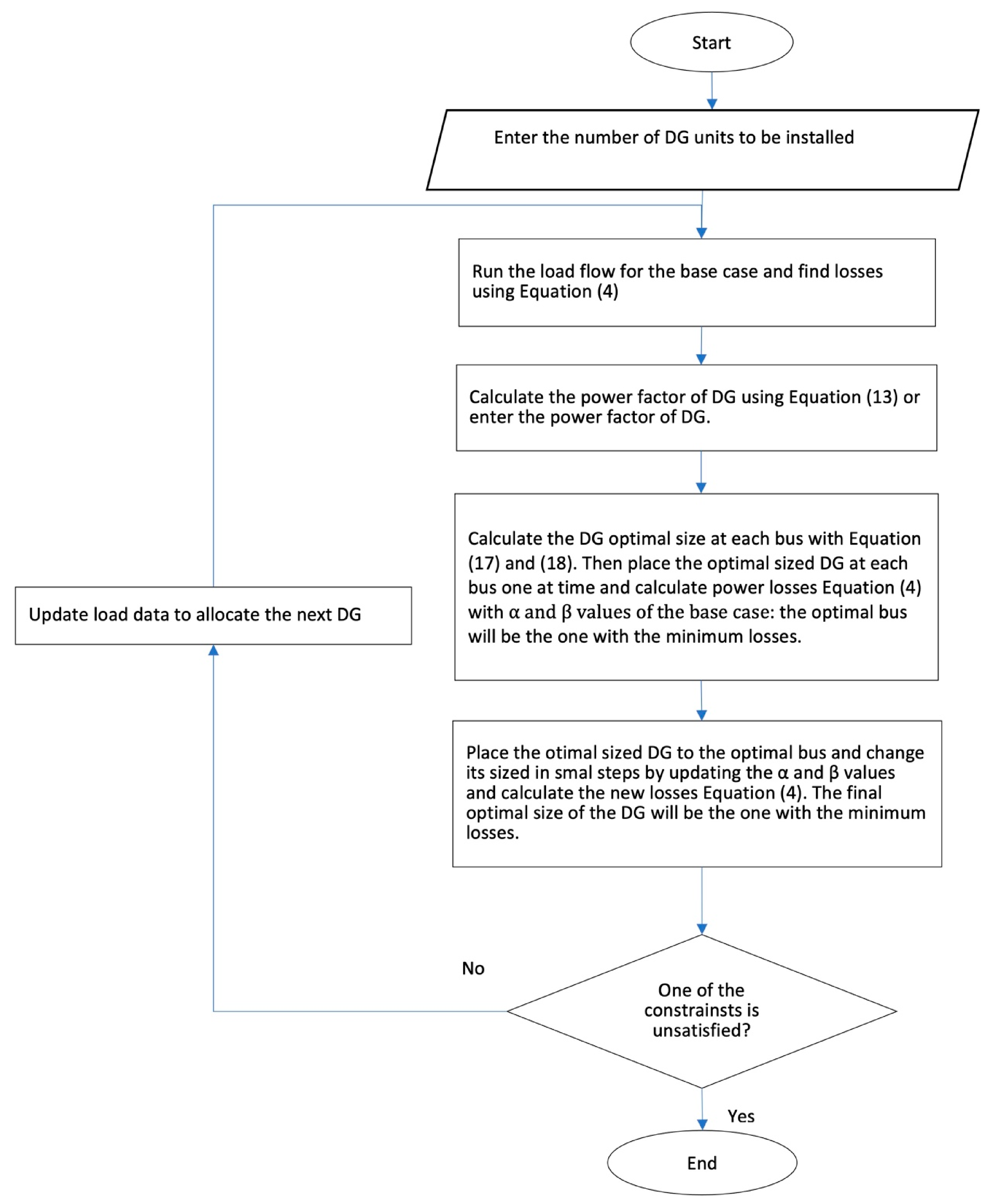
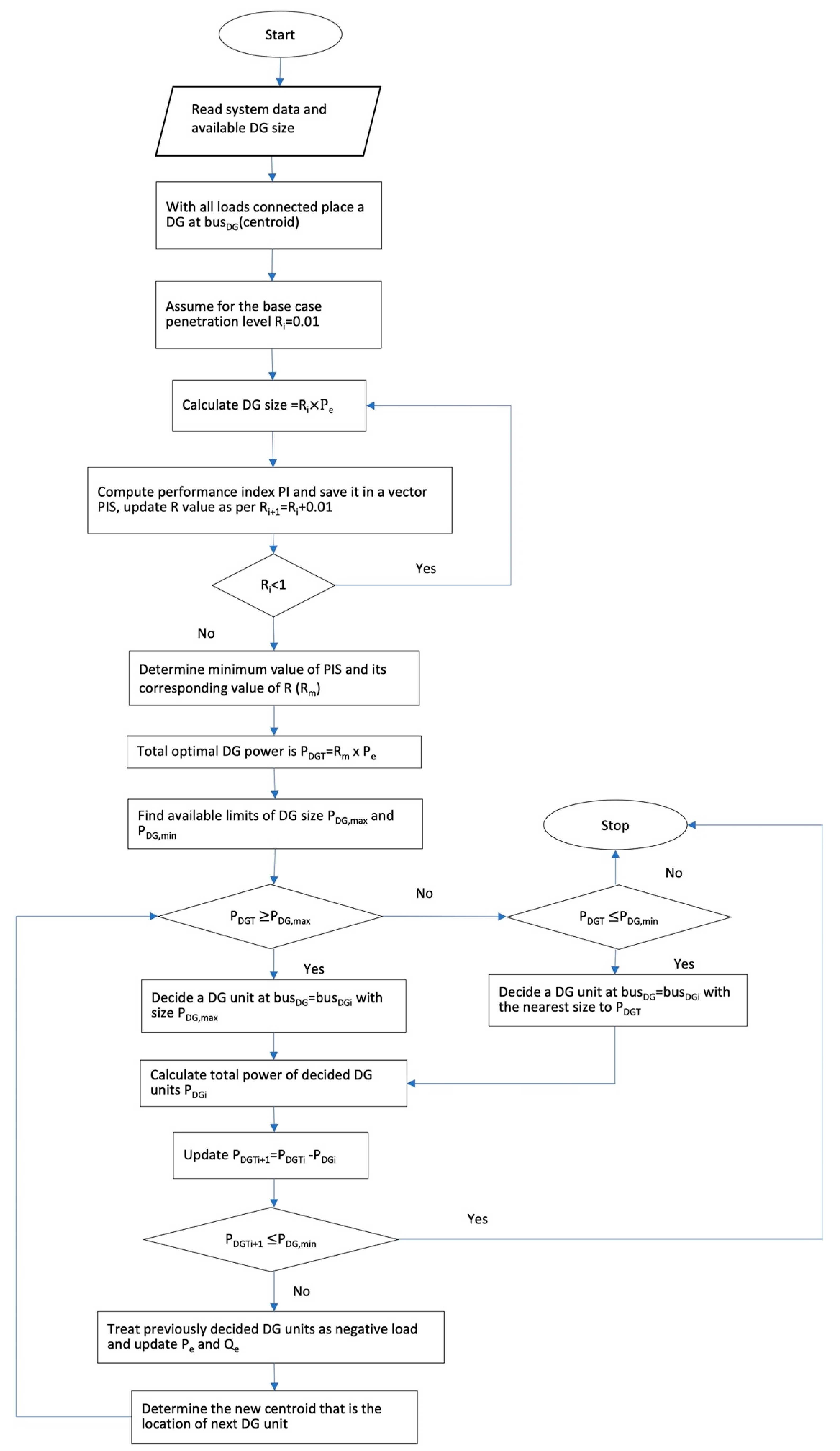
2.1.1. Exact Loss Formula

This method is based on the power losses formula, reported as follows [134]:

$$P_L={\displaystyle \sum }_{i=1}^N{\displaystyle \sum }_{j=1}^N\left[{\alpha }_{ij}\left(P_i{P}_j+Q_i{Q}_j\right)+{\beta }_{ij}\left(Q_i{P}_j-P_i{Q}_j\right)\right]$$

(4)

$${\alpha }_{ij}=\frac{r_{ij}}{V_i{V}_j}\cos \left({\delta }_i-{\delta }_j\right)$$

(5)

$${\beta }_{ij}=\frac{r_{ij}}{V_i{V}_j}\sin \left({\delta }_i-{\delta }_j\right)$$

(6)

$$P_i=P_{DGi}-P_{Di}$$

(7)

$$Q_i=Q_{DGi}-Q_{Di}$$

(8)

Rearranging (Equation (4)) using (Equations (7) and (8)):

$$\begin{array}{cc}{P}_L={\displaystyle {\displaystyle \sum }_{i=1}^N}{\displaystyle {\displaystyle \sum }_{j=1}^N}[{\alpha }_{ij}(\hfill & \left(P_{DGi}-P_{Di}\right)P_j+(Q_{DGi}-Q_{Di})Q_j+{\beta }_{ij}\left((Q_{DGi}-Q_{Di}\right)P_j\hfill \\ & -(P_{DGi}-P_{Di})Q_j)]\hfill \end{array}$$

(9)

(Equation (9)) then will be minimized imposing

$$\frac{\partial P_L}{\partial P_i}=2{\displaystyle \sum }_{i=1}^N\left({\alpha }_{ij}{P}_j-{\beta }_{ij}{Q}_j\right)=0$$

(10)

(Equation (11)) is derived from (Equation (10)):

$$P_i=\frac{1}{{\alpha }_{ii}}\left[{\beta }_{ii}{Q}_i+{\displaystyle \sum }_{j=1,j\ne 1}^N\left({\alpha }_{ij}{P}_j-{\beta }_{ij}{Q}_j\right)\right]$$

(11)

Finally, using (Equation (7)), the following equation is obtained:

$$P_{DGi}=P_{Di}+\frac{1}{{\alpha }_{ii}}\left[{\beta }_{ii}{Q}_i-{\displaystyle \sum }_{j=1,j\ne 1}^N\left({\alpha }_{ij}{P}_j-{\beta }_{ij}{Q}_j\right)\right]$$

(12)

The base algorithm, applied to the Exact loss formula methods, contemplates computing the power losses in the distribution network before placing the DGs simply running (Equation (4)). The second step is calculating the DG optimal size at each bus based on (Equation (12)). The third and fourth steps realize a bus priority list, ordered from the bus with the lowest power loss to the higher one, after substituting at each bus per time the DG unit with its optimal size and calculating the related power losses. The optimal locations to place the optimal sized DGs are selected from the priority list.

In the literature, analytical techniques, based on the exact loss formula, try to improve the computational efficiency when the impedance matrix or Jacobian matrix when large-scale distribution networks are considered [24], to adapt these calculations to the different type of DGs, because the particular nature of the DG has decisive influence on the total power losses of the networks. Duong et al. [135] propose an iterative analytical method that can be applied to generators capable of delivering both active and reactive power. The different types of generators with their constitutive equations are listed in Table 2. At each iteration, (Equation (4)) is minimized by applying the equations in Table 2 for each generator. For each node i, (Equation (4)) must be solved twice: the first to calculate the base case and the second to establish the generator size. To identify the correct power factor, the method proposes two types of approaches: the first, being faster, consists in matching the power factor of each generator to the overall power factor of the loads (Equation (13))

$$P{F}_{DGi}=P{F}_D$$

(13)

where the overall loads power factor is expressed as

$$P{F}_D=\frac{P_D}{\sqrt{P_D^2+Q_D^2}}$$

(14)

$$P_D={\displaystyle \sum }_{i=1}^n{P}_{Di} Q_D={\displaystyle \sum }_{i=1}^n{Q}_{Di}$$

(15)

The generator power factor is expressed as

$$P{F}_{DGi}=\frac{P_{DGi}}{\sqrt{P_{DGi}^2+Q_{DGi}^2}}$$

(16)

The second case, instead, involves an iterative calculation, as the power factors of some DGs are made to vary by small steps around the power factor value of the combined loads. Finally, the power factor values are compared with the constitutive equations in the table and the values that produce lower power losses are chosen. Figure 1 shows the flow chart which summarizes the logical steps of the proposed method.

Table 2. Constitutive equations for different generator types.

Type 1 DG Injects Active and Reactive Power	Type 2 DF Injects Active and Consumes Reactive Power	Type 3 DG Injects Only Active Power	Type 4 DG Injects Reactive Power
$$P_{DGi}=\frac{{\alpha }_{ii}\left(P_{Di}+a{Q}_{Di}\right)-X_i-a{Y}_i}{a^2{\alpha }_{ii}+{\alpha }_{ii}}$$ (17) where $$Q_{DGi}=a{P}_{DGi}$$ (18) $$X_i={\sum }_{j=1; j\ne i}^n\left({\alpha }_{ij}{P}_j-{\beta }_{ij}{Q}_j\right)$$ (19) $$Y_i={\sum }_{j=1;j\ne i}^n\left({\alpha }_{ij}{Q}_j+{\beta }_{ij}{P}_j\right)$$ (20) $$a=\left(sign\right)\tan \left({\cos }^{-1}\left(P{F}_{DG}\right)\right)$$ (21) For DG injecting reactive power $sign=+1$	The constitutive equations are the same of Type 1 generators, the only difference is in (Equation (20)). For DG absorbing reactive power $sign=-1$	$$P_{DGi}=P_{Di}-\frac{1}{{\alpha }_{ii}}{\sum }_{j=1; j\ne i}^n\left({\alpha }_{ij}{P}_j-{\beta }_{ij}{Q}_j\right)$$ (22)	$$Q_{DGi}=Q_{Di}-\frac{1}{{\alpha }_{ii}}{\sum }_{j=1; j\ne i}^n\left({\alpha }_{ij}{Q}_j-{\beta }_{ij}{P}_j\right)$$ (23)

Table 2. Constitutive equations for different generator types.

Type 1 DG Injects Active and Reactive Power	Type 2 DF Injects Active and Consumes Reactive Power	Type 3 DG Injects Only Active Power	Type 4 DG Injects Reactive Power
$$P_{DGi}=\frac{{\alpha }_{ii}\left(P_{Di}+a{Q}_{Di}\right)-X_i-a{Y}_i}{a^2{\alpha }_{ii}+{\alpha }_{ii}}$$ (17) where $$Q_{DGi}=a{P}_{DGi}$$ (18) $$X_i={\sum }_{j=1; j\ne i}^n\left({\alpha }_{ij}{P}_j-{\beta }_{ij}{Q}_j\right)$$ (19) $$Y_i={\sum }_{j=1;j\ne i}^n\left({\alpha }_{ij}{Q}_j+{\beta }_{ij}{P}_j\right)$$ (20) $$a=\left(sign\right)\tan \left({\cos }^{-1}\left(P{F}_{DG}\right)\right)$$ (21) For DG injecting reactive power $sign=+1$	The constitutive equations are the same of Type 1 generators, the only difference is in (Equation (20)). For DG absorbing reactive power $sign=-1$	$$P_{DGi}=P_{Di}-\frac{1}{{\alpha }_{ii}}{\sum }_{j=1; j\ne i}^n\left({\alpha }_{ij}{P}_j-{\beta }_{ij}{Q}_j\right)$$ (22)	$$Q_{DGi}=Q_{Di}-\frac{1}{{\alpha }_{ii}}{\sum }_{j=1; j\ne i}^n\left({\alpha }_{ij}{Q}_j-{\beta }_{ij}{P}_j\right)$$ (23)

The results of the proposed method show how DGs, capable of delivering both real and reactive power, reduces losses more than DGs which deliver only active power. Moreover, it was shown also that correct selection of the power factor, in case of DGs capable delivering both active and reactive power, has a crucial role in power loss reduction.

Duong et al. [136] showed two analytical approaches to identify optimal size and best siting of renewable DGs, taking into account the time-varying demand (Figure 2) and the outputs of different RER-based DGs (Figure 3). The first proposed method, called A1, is based on the Elgered loss equation and is applied in the solution of two case studies. In the first case, the method is applied to identify the best positioning and the corresponding size of the generators, assuming as a hypothesis to size the generators on the peak of demand and therefore not to allow any type of regulation. In the second case, however, the variable nature of the demand is considered, and the different characteristics of each DG are taken into account.

Four scenarios are, therefore, formulated in which three different types of generators are considered: a PV-based DG and a Wind-based DG, considered with their hourly output curves, but considered as non-dispatchable resources, and finally a Biomass-based DG, considered both as a dispatchable and as a non-dispatchable resource. The algorithm used for the solution of the optimization problem is shown in Figure 4.

The second method proposed, called A2, is based on the “branch current loss formula”. The active and reactive power can therefore be expressed as

$$P_{DGk}=-\left|V_k\right|\frac{{\sum }_{i=1}^k{I}_{ai}{R}_i}{{\sum }_{i=1}^k{R}_i}$$

(24)

$$Q_{DGk}=-\left|V_k\right|\frac{{\sum }_{i=1}^k{I}_{ri}{R}_i}{{\sum }_{i=1}^k{R}_i}$$

(25)

The Power loss reduction can be expressed as

$$∆P_{loss}=\frac{{\left({\sum }_{i=1}^k{I}_{ai}{R}_i\right)}^2}{{\sum }_{i=1}^k{R}_i}+\frac{{\left({\sum }_{i=1}^k{I}_{ri}{R}_i\right)}^2}{{\sum }_{i=1}^k{R}_i}$$

(26)

The same algorithm as per Figure 4 can be applied for method A2 by calculating the active power and reactive power as per (Equation (24)) and (Equation (25)), respectively, and using (Equation (26)) as objective function to minimize.

The proposed methods offer near-optimum results, as these numerical results have been compared with the exhaustive load flow solution. The authors also found that for non-dispatchable DGs it is difficult to reach the optimal loss reduction in peak conditions. The strengthen of these methods is that they can easily be implemented in practice in a smart grid scheme. The efforts to account the time-variability of renewable DGs and a dynamic load demand in the analytical formulas have a relevant impact on the applicability of these methods in future scenarios, where the penetration of RER-based DGs is the future driver for the evolution of distributed networks. Different attempts can be already found in literature.

Elmitwally [137] presents a new Analytical method (A5) based on the concept of the load centroid. As in an electrical distribution network it is highly improbable to be able to position the generator in the immediate vicinity of the load, as it is enslaved to different loads, the concept of load centroid then proposes to find the electrical equivalent of what in mechanics is the center of gravity, that is the center of action of a single DG within which the loads it serves are located. Two methods for calculating the load centroid were examined, both are based on the estimate of the Performance index (PI) (Equation (27)), which, by combining the value of the active power loss and the Average Node Voltage Deviation ($ANVD)$ (Equation (28)) multiplied by a selective weighting factor $K$, allows to identify the ideal position for the DG location.

$$PI=P_{loss}+K ANVD$$

(27)

$$ANVD=\left|1-\frac{{\sum }_n{V}_n}{N_B}\right|$$

(28)

In Figure 5 and Figure 6, the flow charts of the first and second method, respectively, are presented. Once the load centroid has been found, one can then proceed with the algorithm proposed by the author to identify the different sizes of each generator by iteratively calculating the new load centroid after each positioning of each DG. In Figure 7, the logical scheme of the proposed algorithm is presented.

Hung et al. in [44] proposed analytical expressions to locate and size different renewable DG units and calculate the optimal power factor for each unit, considering the uncertainties of demand and DGs output to minimize the energy losses.

Hung et al. [45] described the functioning of a dispatchable renewable DG (a Photovoltaic based DG with its battery storage), where the uncertainties of demand and generation have been accounted by using a self-correction algorithm. The size of the DG is calculated by minimizing a multi-objective function, which accounts power losses and voltage deviation. The power losses and voltage deviation multi-objective function are also used in [42], where it is minimized to find the optimal capacity of PV units in different load scenarios, matching always the uncertainties of demand and outputs.

2.1.2. Loss Sensitivity Factor

This method has been widely used to solve the capacitor allocation problem [138], and its strengthen is a reduction of the solution space by means of a linearization process of v 5 respect to the initial operating point.

$$\frac{\partial P_L}{\partial P_i}=2{\displaystyle \sum }_{i=1}^N\left({\alpha }_{ij}{P}_j-{\beta }_{ij}{Q}_j\right)$$

(29)

The steps of the method consist in solving the (Equations (4) and (13)) without DGs to estimate the sensitivity factors at each bus; then the buses, similarly to what done in the exact loss algorithm, are ranked in a priority list.

The top ranked buses are used first to locate the DGs, and the optimal DGs capacity is found increasing the capacity until lowest system losses are obtained by solving (Equation (29)).

The process reaches the end when all the bus are used and the bus which results in minimum power losses is selected as optimal DG location. The drawbacks of this method result in several iterations in calculating the power losses, which can limit the spread of this method in problem scale-out [38].

Kashem et al. [139] applied the sensitivity analysis on active and reactive power to calculate the site and size of DGs. The results show not only a benefit in enhancing the penetration of DGs, but also that the decrease in power losses is much higher if a proper DG planning is performed.

Mirzaei et al. [140] considered different RER based DGs and the optimum capacity was calculated taking into account a hybrid analytical technique, based on the sensitivity analysis, combined with the continuous power flow method.

In fact, the method proposes to insert the maximum loadability (λ_max) in the calculation of the active and reactive power to take into account the collapse point (CP) of the voltage. If considered the Voltage-Loading Parameter (λ) dependency, the stability of the voltage is a function of the current circulating in the branch up to the point of collapse of the voltage. The presence of a DG causes an increase in voltage at the bus, as injecting active power into the bus results in a decrease in reactive power, with a consequent extension of the collapse point towards higher load values. Therefore, applying the Voltage-Loading Parameter (λ), the trend of the active, and reactive power become, respectively,

$$P_D=P_D^{oi}+\lambda P_D^{CPF}$$

(30)

$$Q_D=Q_D^{oi}+\lambda Q_D^{CPF}$$

(31)

Thus, rearranging (Equations (30)) and (31) with (Equation (7)) and taking into account the variability of the power factor as a function of the different types of generators, we obtain the following constitutive equations:

(1) Generators capable of injecting only active power:

$$P_{DGi}=\left(P_{Di}^{oi}+{\lambda }_i{P}_{Di}^{CPF}\right)+\frac{1}{{\alpha }_{ii}}\left[{\beta }_{ii}{Q}_i-{{\displaystyle \sum }}_{j=1,j\ne i}^N\left({\alpha }_{ij}{P}_j-{\beta }_{ij}{Q}_j\right)\right]$$

(32)

(2) Generators able to input only reactive power:

$$Q_{DGi}=\left(Q_{Di}^{oi}+{\lambda }_i{Q}_{Di}^{CPF}\right)+\frac{1}{{\alpha }_{ii}}\left[{\beta }_{ii}{P}_i-{{\displaystyle \sum }}_{j=1,j\ne i}^N\left({\alpha }_{ij}{Q}_j-{\beta }_{ij}{P}_j\right)\right]$$

(33)

(3) Generators with mixed power factor:

$$\begin{array}{cc}\hfill P_{DGi}=\left(P_{Di}^{oi}+{\lambda }_i{P}_{Di}^{CPF}\right)& -\left[\frac{1}{{\alpha }_{ii}\times \left(1+\sqrt{\frac{1-P{F}^2}{P{F}^2}}\right)}\right]\hfill \\ & \times [{\alpha }_{ii}\times \sqrt{\frac{1-P{F}^2}{P{F}^2}}\left(Q_{Di}^{oi}+{\lambda }_i{Q}_{Di}^{CPF}\right)\hfill \\ & -{{\displaystyle \sum }}_{j=1,j\ne i}^N({\alpha }_{ij}\left(P_j+\sqrt{\frac{1-P{F}^2}{P{F}^2}}{Q}_j\right)\hfill \\ & -{\beta }_{ij}\left(\sqrt{\frac{1-P{F}^2}{P{F}^2}}{P}_j-Q_j\right)\left)\right]\hfill \end{array}$$

(34)

Therefore, starting from the aforementioned mathematical treatment, the authors propose the following solution algorithm in Figure 8.

The results show a decrease in power losses and an increase of the network voltage stability.

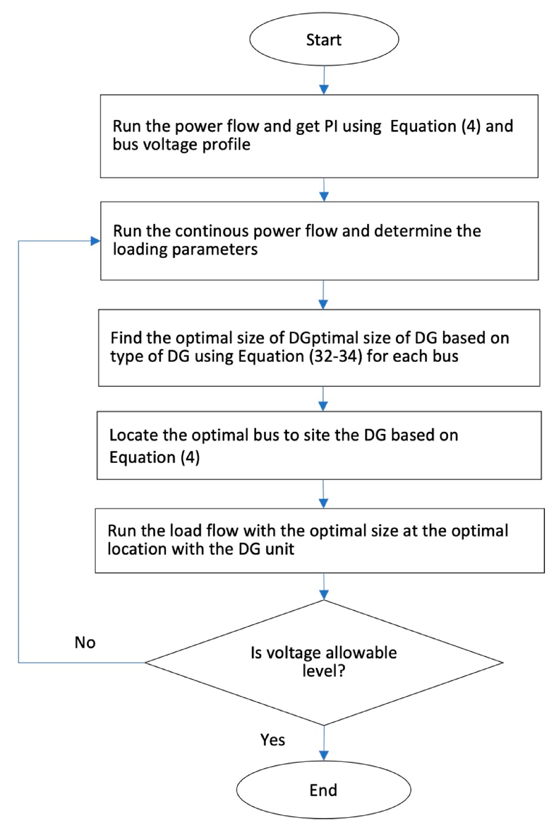
2.2. Optimal Power Flow

The optimal power flow approach was discussed firstly by Carpentier in 1962 [141], and its main scope is to define the optimal operating state to instantaneously operate and control a power network under constrained conditions. The OPF method in the “reverse loadability” approach is able to size the DGs capacity and to find their optimal locations to minimize the power losses and decrease the operational cost [11]. From 1962, a variety of OPF versions have been proposed so far. Mathematically, the OPF models can be expressed as an objective function (Equation (1)), subjected to specific constraints as per (Equations (2) and (3)).

Mahmoud et al. [41] proposed a new mixed analytical-OPF method which dramatically decrease the computational time for solving the optimization problem of the correct design of a distribution network grid. The method exploits the real power loss (RPL) calculation scheme proposed in the analytical solver called Efficient Analytical (EA) Method. The RPL calculated as in (Equation (35)) requires solving the load flow equation only once.

$$\begin{array}{cc}RP{L}_{DG}={{\displaystyle \sum }}_{j\notin BDG}& \frac{r_j}{V_j^2}\left(P_j^2+Q_j^2\right)\hfill \\ & +{{\displaystyle \sum }}_{j\in BDG}\frac{r_j}{V_j^2}({\left(P_j-{{\displaystyle \sum }}_{i\in NDG}{S}_{ij}{P}_{DGi}\right)}^2\hfill \\ & +{\left(Q_j-{{\displaystyle \sum }}_{i\in NDG}{S}_{ij}{Q}_{DGi}\right)}^2)\hfill \end{array}$$

(35)

where S represents the complex power as binary matrix (NDGxBDG) defined as follows:

$$S_{ij}=\left\{\begin{array}{cc}1,\hfill & if S_{DGi} passes through branch j\hfill \\ 0,\hfill & otherwise\hfill \end{array}\right\}$$

(36)

It is therefore no longer necessary to recalculate the power losses before and after the positioning of the generators, as the second term of (Equation (35)) already takes into account the influence that the addition of the generator would have on the power loss in the branch. The first term, on the other hand, of (Equation (35)) remains constant and, therefore, takes into account the base case. From (Equation (35)) it is possible to obtain the (Equation (36)), which will become the objective function of the analytical solver.

$$\begin{array}{cc}RPL{R}_{DG}={{\displaystyle \sum }}_{j\in BDG}& \frac{r_j}{V_j^2}(2{{\displaystyle \sum }}_{i\in NDG}{S}_{ij}{P}_{DGi}\left(P_j+Q_j{{\displaystyle \sum }}_{i\in NDG}{S}_{ij}\sqrt{\frac{1-P{F}_{DGi}^2}{P{F}_{DGi}^2}}\right)\\ & -{{\displaystyle \sum }}_{i\in NDG}{S}_{ij}{P}_{DGi}^2\left(1+{{\displaystyle \sum }}_{i\in NDG}{S}_{ij}\frac{1-P{F}_{DGi}^2}{P{F}_{DGi}^2}\right))\end{array}$$

(37)

The optimization process will be calibrated on the nature of the generator by returning the value of the sizes of the generators positioned in each branch of the network. In the case of generators with a known power factor, the objective function becomes the one in (Equation (37)), while in case of unspecified power factors the solver imposes the condition in (Equation (38)).

$${\left.\frac{\partial RPL{R}_{DGs}}{\partial P_{DGm}}\right|}_{P_{DGi=}{P}_{DGi}^{opt}}=0$$

(38)

$${\left.\frac{\partial RPL{R}_{DG}}{\partial P_{DGm}}\right|}_{P_{DGi=}{P}_{DGi}^{opt}, Q_{DGi}=Q_{DGi}^{opt}}={\left.\frac{\partial RPL{R}_{DG}}{\partial Q_{DGm}}\right|}_{P_{DGi=}{P}_{DGi}^{opt}, Q_{DGi}=Q_{DGi}^{opt}}$$

(39)

As the number of possible combinations (N_C) Generators-Nodes in the network is equal to

$$N_C=\frac{N_B!}{N_{DG}!\left(N_B-N_{DG}\right)!}$$

(40)

an estimated RPLR is formulated to find the best placement. The proposed algorithm scheme for the EA method is represented in Figure 9. The EA method can be used in combination with the OPF method. In this case, the EA method is used to calculate the correct size of the generators, it will be the task of the OPF solver to find the optimal placement of the generators by verifying that they respect the network constraints. Figure 10 shows the complete scheme of the combined EA-OPF method.

Abdi et al. [142] proposed a review of the different approaches, differentiating them by objective functions, constraints, variables, mathematical formulation and solution algorithms. The grid topology, as well as the control strategy and the different equipment employed in the studied network, affect dramatically the results and the performance of the OPF method used, so it is fundamental to choose the correct OPF approach to solve the optimization problem.

The strength of the OPF method lies in its adaptation for the implementation in different network topologies and in its ability to incorporate in the mathematical formulation the new technologies constitutive equations of intelligent networks, thus allowing to update the mathematical model with the values of the electrical variables, measured in real time.

OPF can be extended on different energy carriers, describing more accurately the energy flow and conversion along different processes, strictly interconnected by means of the creations of an Energy Hub (EH) [143]. Despite OPF has a markable flexibility in modelling networks behaviors, there is still space for improvements, for example, to better integrate the optimal economic point with the technical optimal one, accounting the curtailment cost related to various operation intervals and the impact of the market on reactive power cost. Furthermore, the EH is not completely developed, specially it is not applied to smart grids yet, as well as the Optimal Energy Flow method. Finally, it is necessary to better modelling uncertainties, implementing new methods, as done in [144,145,146] to overcome the computational effort of the Monte Carlo method, used to model the stochastic nature of renewable power generation and the uncertainties of the demand-side management [142].

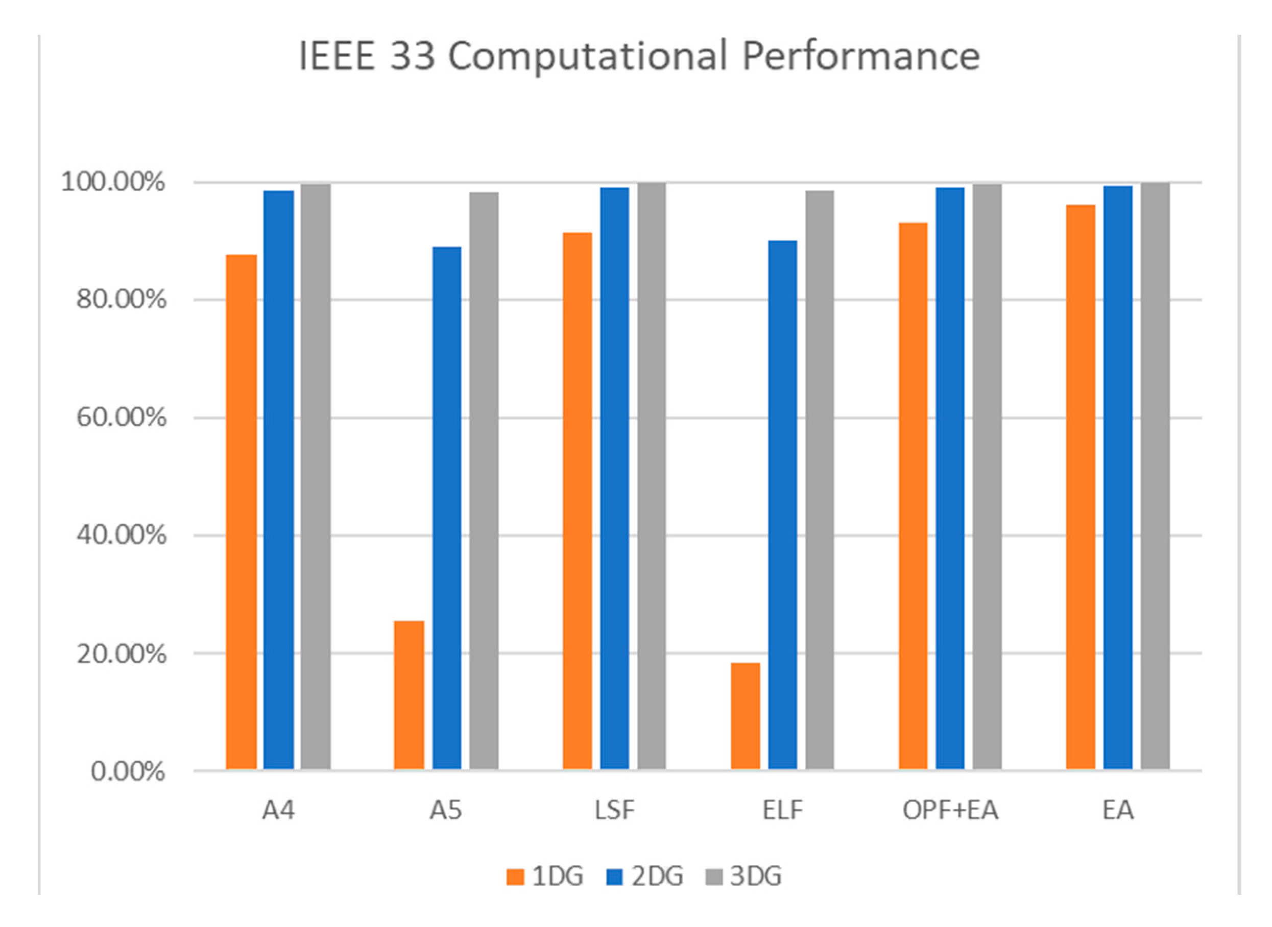
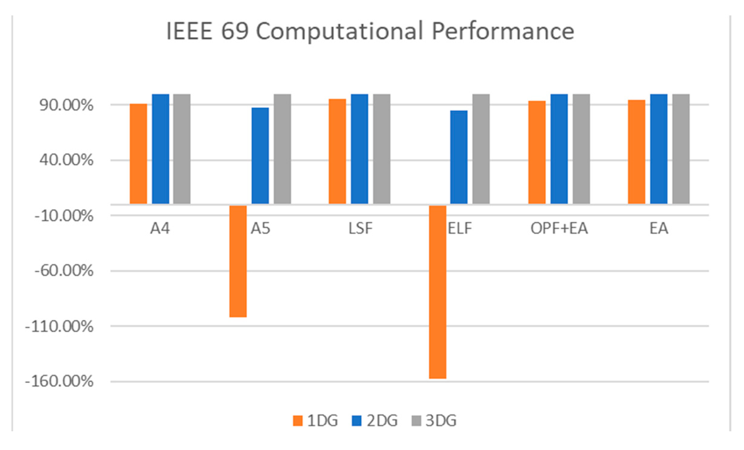
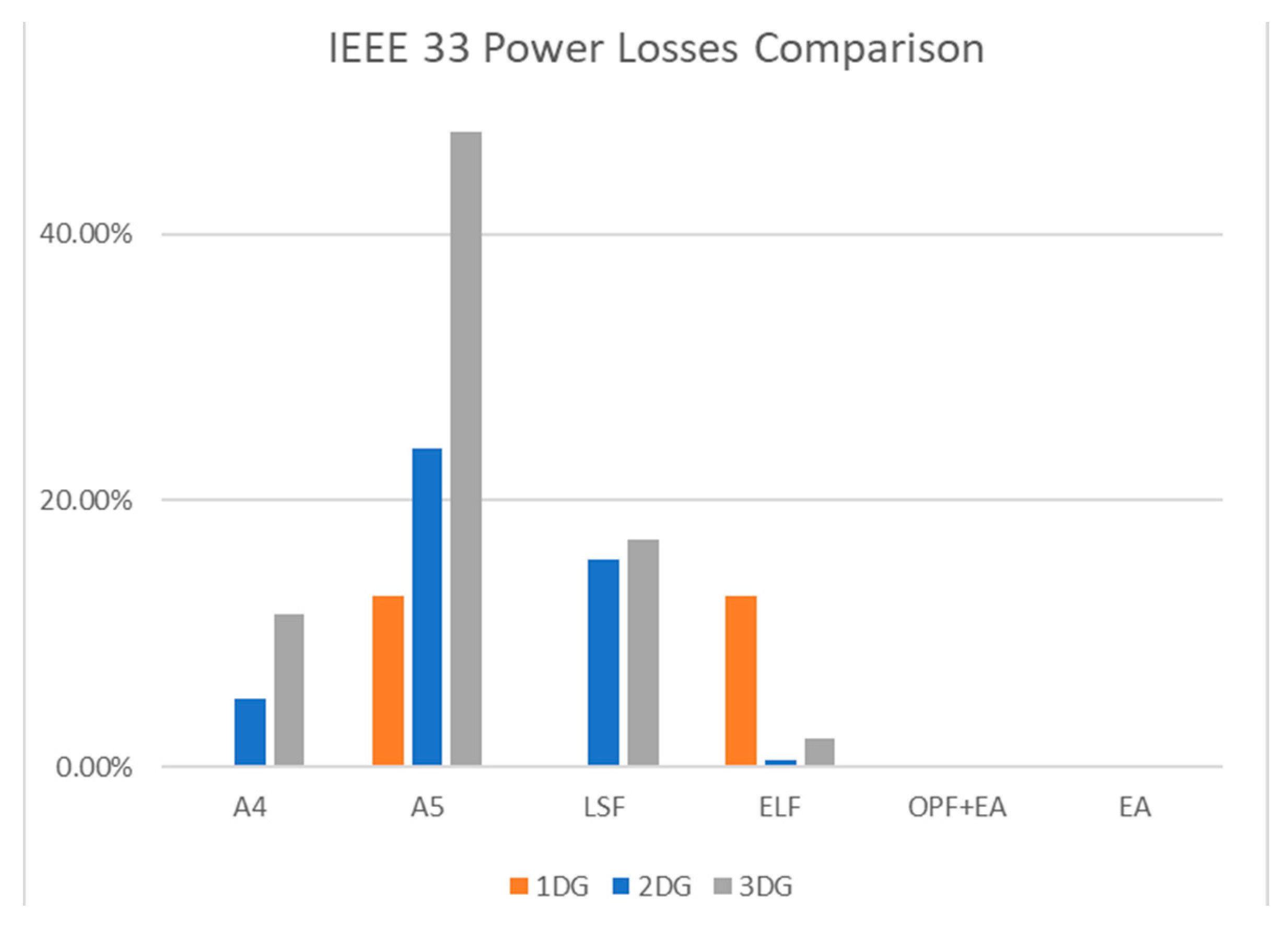
2.3. Numerical Results

Considering the different nature of all optimization methods and the different grids used in literature to test the algorithms effectiveness, it is hard to establish a benchmark to evaluate the performance of the methods used to solve the optimization problem. For this reason, to validate the different approaches, we chose two grid models: the IEEE 33 [147] and IEEE 69 [148] Bus Test Systems and, on these two grids, the Analytical Techniques and the OPF method have been applied to compare their different performance.

The results, obtained by solving the two network configurations by positioning a different number of generators each time up to a maximum of 3, are shown in

Table 3. Optimization methods comparison—DG capable to supply active power.

Bus Test System	Method	N. DG	Optimal Bus				Optimal Size [kw]				Power Loss [kW]	CPU Time [s]
IEEE 33	Analytical method A3 [38]	1	6				2490				111.24	0.09
	Analytical method A4 [135]		6				2601				111.10	0.16
	Analytical method based on Loss Sensitivity factor [135]		18				743				146.82	0.11
	Analytical method based on Exhaustive Loss Factor [135]		6				2601				111.10	1.06
	Analytical method A5 [137]		30				1500				125.21	0.97
	Efficient analytical method [41]		6				2530				111.07	0.05
	Efficient analytical method combined with OPF [41]		6				2590				111.02	0.09
	OPF [41]		6				2590				111.02	1.30
	Analytical method A4 [135]	2	6		14		720		1800		91.63	0.27
	Analytical method based on Loss Sensitivity factor [135]		18		33		720		900		100.69	0.18
	Analytical method based on Exhaustive Loss Factor [135]		12		30		1020		1020		87.63	2.03
	Analytical method A5 [137]		30		25		1500		1000		107.95	2.23
	Efficient analytical method [41]		13		30		844		1149		87.172	0.11
	Efficient analytical method combined with OPF [41]		13		30		852		1158		87.17	0.15
	OPF [41]		13		30		852		1158		87.17	20.2
	Analytical method A4 [135]	3	6	12		31	900	900		720	81.05	0.4
	Analytical method based on Loss Sensitivity factor [135]		18	33		25	720	810		900	85.07	0.23
	Analytical method based on Exhaustive Loss Factor [135]		13	30		24	900	900		900	74.27	3.06
	Analytical method A5 [137]		30	25		24	1500	1000		220	107.35	3.26
	Efficient analytical method [41]		13	24		30	798	1099		1050	72.787	0.37
	Efficient analytical method combined with OPF [41]		13	24		30	802	1091		1054	72.79	0.41
	OPF [41]		13	24		30	802	1091		1054	72.70	202
IEEE 69	Analytical method A3 [38]	1	61				1810				83.4	0.54
	Analytical method A4 [135]		61				1900				81.33	0.28
	Analytical method based on Loss Sensitivity factor [135]		65				1520				109.77	0.15
	Analytical method based on Exhaustive Loss Factor [135]		61				1900				81.33	7.75
	Analytical method A5 [137]		61				1900				83.25	6.09
	Efficient analytical method [41]		61				1878				83.23	0.16
	Efficient analytical method combined with OPF [41]		61				1870				83.23	0.2
	OPF [41]		61				1870				83.23	3.01
	Analytical method A4 [135]	2	61		17		1700		510		70.3	0.52
	Analytical method based on Loss Sensitivity factor [135]		65		27		1440		540		98.74	0.3
	Analytical method based on Exhaustive Loss Factor [135]		61		17		1700		510		70.3	15.53
	Analytical method A5 [137]		61		64		1900		20		83.23	12.3
	Efficient analytical method [41]		61		17		1795		534		71.68	0.45
	Efficient analytical method combined with OPF [41]		61		17		1781		531		71.68	0.5
	OPF [41]		61		17		1781		531		71.68	101
	Analytical method A4 [135]	3	61	17		11	1700	510		340	68.38	0.71
	Analytical method based on Loss Sensitivity factor [135]		65	27		61	1360	510		510	58.57	0.52
	Analytical method based on Exhaustive Loss Factor [135]		61	17		11	1700	510		340	68.38	23.16
	Analytical method A5 [137]		61	64		21	1900	20		470	72.65	17.3
	Efficient analytical method [41]		61	18		11	1795	380		467	69.62	1.62
	Efficient analytical method combined with OPF [41]		61	18		11	1719	380		527	69.43	1.66
	OPF [41]		61	18		11	1719	380		527	6943	6655

. By hypothesis, in this first case, those generators only deliver active power. The OPF method in [41] is used as benchmark on the basis of which all the analyses have been carried out, regarding the performance of the other algorithms used to solve the optimization problem. The OPF method can completely solve any network configuration by returning the optimal size and site values of the DGs. The main drawback lies in the excessive computational time required. For example, for the IEEE 33 network configuration, the time required varies from 1.30 s, to solve the system by positioning only one DG, up to 202 s, required to solve the network with 3 DGs. The computational effort grows even more if complex network configurations have to be considered, such as IEEE 69 with 3 DGs. In this case the time required by the CPU amounts to 6655 s. In [41], the authors also present a mixed method, which combines the OPF method with an analytical method, based on Real Power Loss Reduction (RPLR). With this new approach, indeed, the analytical method finds the best location for DGs and finally the OPF algorithm is employed to solve the optimization sizing problem. This new method has the advantage of considerably reducing the computational effort, even with complex network configurations, for example the IEEE 69 configuration with 3 DGs is solved in 1.66 s, instead of the previous 6655 s, required by applying only the OPF method. The combined OPF method also returns the same size and position values to the nodes of the DGs, identified by the OPF method.

Hung et al. [135] considered an iterative Analytical method (A4), which has considerable advantages under the computational point of view. It is completely comparable with the combined OPF method, however it has the disadvantage of presenting a solution which is trapped in local optimum, as evidenced by the different sizes and different nodes, identified in generators placement in IEEE 33 network configuration with three DGs and 2 DGs together with the IEEE 69 network configuration with 3 DGs.

Elmitwally [137] presented a method that has a computational time 20 times greater than the A4 analytical method in the IEEE 69 network configuration at three DGs, however, it is still more advantageous than the OPF method.

Even in this case, the method is very sensitive to local optimal solutions, in fact in almost all the network configurations the method is trapped in optimal locals, as evidenced by the higher power losses calculated, compared to global optimal solutions. Only in the IEEE 69 network configuration with 1 DG it has managed to produce a solution comparable to that of the other methods.

Table 4. Optimization methods comparison—DG capable to supply active and reactive power.

Bus Test System	Method	N. DG	Optimal Bus	Optimal Size [kVA]	Power Loss [kW]	Power Factor
IEEE 33	Analytical method A4 [135]	1	6	3107	67.9	0.82
		2	6	2195	44.39	0.82
			30	1098
		3	6	1098	22.29	0.82
			30	1098
			14	768
IEEE 69	Analytical method A4 [135]	1	61	2243	22.62	0.82
		2	61	2195	7.25	0.82
			17	659
		3	61	2073	4.95	0.82
			17	622
			50	829
IEEE 33	Efficient analytical method combined with OPF [41]	1	6	2558	67.86	0.82
		2	13	846	28.50	0.90
			30	1138		0.73
		3	13	794	11.74	0.90
			24	1070		0.90
			30	1030		0.71
IEEE 69	Efficient analytical method combined with OPF [41]	1	61	1828	23.17	0.82
		2	61	1735	7.20	0.81
			17	522		0.83
		3	11	495	4.27	0.81
			18	379		0.83
			61	1674		0.81
IEEE 69	Analytical method A1 [134,136]	1	61	1844.4	21.08	0.814
	Analytical method A2 [136,149]	1	61	1844.3	21.11	0.825

shows the results obtained by solving the same network configurations presented in Table 3, assuming the DGs capable to deliver both active and reactive power. The difficulty of the A4 analytical method immediately emerges to free itself from local optimal solutions even in this situation, reporting higher power losses than the combined OPF method, except for the IEEE 69 one DG configuration. In this case, while managing both methods to identify the exact Bus where to place the generator, the combined OPF method has a loss of 23.17 kW, slightly higher than the 22.62 kW of the A4 method. The reason lies in the nominal power of the generator identified by the methods. In the case of the combined OPF method it is 1828 kVA, lower than the 2243 kVA of the A4 method. However, both generators, identified by the two methods, have the same power factor.

In [136], the proposed analytical methods are based on the Elgerd’s loss formula, called Analytical method A1, and on the branch current loss formula, called Analytical method A2. The results, obtained by applying these two methods to the IEEE 69 network configuration with one DG, are completely comparable to those obtained by the combined OPF method.

Making a comparison with the CPU’s Time data, it is evident that the A4, EA, LSF, and OPF combined with EA methods are the fastest methods. In Figure 11 and Figure 12, the relative computational times are represented, respectively, in IEEE 33 and in IEEE 69 case studies, i.e., the computational time required by each method to find a solution compared to the time needed by the OPF method in [41] as base case. In all configurations, they guarantee convergence in almost half the time required for the OPF method. In the case study IEEE 33 Figure 11 the A4 method allows a time saving compared to the OPF method equal to 87.69%, 98.66%, and 99.80%, respectively, in the case of placement of 1 DG, 2 DG, and 3 DG. The OPF combined with EA method, on the other hand, in the case of placement of 1 DG guarantees a computational saving of 93.08%, 99.26% in the case of 2 DG and 99.80% in the case of 3 DG. The EA and LSF methods, on the other hand, are the methods that compete for the primacy relative to the speed of convergence. The EA method is the fastest method in the IEEE 33 case study in the 1 DG and 2 DG configurations going to convergence with a computational time saving of 96.15% and 99.46%, respectively, while in the 3 DG configuration the fastest method turns out to be the LSF saving 99.89 of the Computation time.

In the IEEE 69 Figure 12 case study, on the other hand, the method that achieves convergence in the shortest possible time is the LSF method. However, the gap between LSF and EA in this case study is still small, the computational time saved is 94.68% for the EA method and 95.02% for the LSF method in the 1 DG configuration, 99.55% for the EA method and 99.70% for LSF in the 2 DG configuration, and finally 99.98% for the EA method and 99.99% for the LSF method. The same trend and almost similar values are also confirmed for the other methods in the IEEE case study 69 Figure 12, thus highlighting a good independence of the convergence speed of these methods from the complexity of the electrical network to be solved.

The relative Power Losses of each method weighted with the Power Losses of the base case in [41] for IEEE 33 case study are represented in Figure 13, while in Figure 14 the weighted Power Losses for IEEE 69 case study are reported. Therefore, going instead to consider the Power Losses values reported in Table 3 and Table 4 and comparing the values in Figure 13 and Figure 14, the OPF combined with EA method is the method that best guarantees an accurate calculation regarding the Power Losses and completely equal to the values obtained with the OPF method. The EA method guarantees values slightly less precise than the OPF combined with EA method, in fact we find an error in the IEEE 33 case study of 0.05% and 0.12% compared to the base case by solving the network with 1 DG and 3 DG, respectively, while in the case study IEEE 69, there is an error of 0.27% solving the network with 3 DG. However, the A4 and LSF methods in the IEEE 69 case study, with generators capable of supplying only real power, guarantee both an error of 2.28%, 1.93%, and 1.51% lower losses compared to the base case respectively in the configurations with 1 DG, 2 DG, and 3 DG. On the other hand, the case of the LSF method is singular, which only in the IEEE 69 3 DG case study records power losses that are 15.64% lower than in the base case, thus demonstrating its high sensitivity to network configurations.

3. Energy Storage Systems

The large penetration of RER DGs, together with the need to enhance the reliability of the grid, as well as the demanding requirements of power and frequency stability are the leading drivers for the emergence of ESS. Despite of the investment cost and, in some cases, the harmful effect on environment are the main limiting factors for a widespread commercialization, a growing in the ESS installed capacity is observed along the years. In 2014, the ESS installed capacity was approximately 140 GW worldwide, in 2018 it was almost 176 GW worldwide [150,151].

In the literature, there exists a general classification of the different ESS systems is as follows: Mechanical energy storage systems, Chemical energy storage systems, Electrochemical energy storage systems, Electrostatic and electromagnetic energy storage systems, and Thermal energy storage systems. Although the number of technical solutions found in literature, the majority of the ESS installed capacity worldwide (96%) is of the Mechanical type, more precisely Pumped hydro energy storage (PHES) and the remaining 4% collects all the other types [152].

The PHES system is the oldest and most mature of all the others. It consists of two basins at different elevations, one basin is higher than the other. The system harnesses the Potential Energy E, stored as difference in elevation between the two basins as per the following relation:

$$E=mg∆h$$

(41)

The potential energy is stored as water pumped to the higher reservoir during off-peak demand. During the peak demand the water is released to the lower reservoir, converting the potential energy in electric energy by means of a hydraulic turbine connected to a generator.

The drawbacks of this solution are mainly related to the cost of the investment, the impact on the environment and the high dependency on the morphology and location of the sites.

Apart the technology maturity, there are other features which can measure the ESS effectiveness. Under a technical point a view, there are the energy density (measured in Wh/kg) and the power density (W/kg), which are two capacity indexes of the storage system; the efficiency expressed both as the efficiency during the charging and discharging phase; lifecycle; and response time. Economically speaking, the success of the ESS depends for the most on its capital cost, the O&M cost, and the environment impact. In [153,154], the authors reviewed the state-of-the-art of different energy storage technologies, investigating how they respond to these different technological and economical parameters. In

Table 5. Classification of different ESS.

Category	Technology	Energy Density [Wh/kg]	Power Density [W/kg]	Overall Efficiency	Lifecycle	Response Time	Capital Cost—Power [$/kW]	Capital Cost—Energy [$/kWh]	Technological Maturity
Mechanical Energy Storage Systems	Pumped hydro energy storage (PHES)	0.5–1.5	0.8–1.1	65–85%	30–50 y	Min	600–2000	5–100	Mature
	Compressed air energy storage (CAES)	30–60	0.65–1.2	40–80%	20–40 y	Min	400–800	2–50	Developed
	Flywheel energy storage (FES)	10–30	400–500	80–99%	20 y	<ms	250–350	1000–5000	Developed
Chemical Energy Storage Systems	Hydrogen storage (HS)	800–10,000	5–500	20–50%	5–15 y	<s	10,000	-	R&D—demonstration precommercial
Electrochemical Energy Storage Systems	Lead-acid battery	50–75	150–300	75–80%	5–15 y	ms	300–600	200–400	Mature
	Nickel-cadmium battery	60–90	150–230	60–65%	10–20 y	ms	500–1500	800–1500	Developed
	sodium-sulfur battery	150–240	90–230	80–90%	10–15 y	ms	1000–3000	300–500	Developed
	Lithium-ion battery	100–200	1000–2000	85–95%	5–15 y	ms	1200–4000	600–2500	Mature
	Vanadium redox battery	35–60	75–150	75–85%	5–15 y	ms	600–1500	150–1000	Developed
	Zinc-bromite battery	75–85	90–110	65–75%	5–10 y	ms	700–2500	150–1000	R&D—demonstration commercial
	Polysulfide bromine battery	15–30	-	65–75%	10–15 y	ms	330–2500	120–1000	R&D—demonstration commercial
Electrostatic and electromagnetic Energy Storage Systems	Supercapacitor energy storage system (SCES)	3–5	2000–5000	97%	20 y	ms	100–300	500–1000	R&D—demonstration precommercial
	Superconducting magnetic energy storage (SMES)	3–25	500–2000	85–99%	20 y	ms	1000–10,000	1000–10,000	R&D—demonstration precommercial
Thermal Energy Storage Systems (TES)		80–250	10–30	30–60%	10–40 y	s-min	200–300	10–50	R&D—demonstration commercial—Developed

, the different ESS technologies are categorized and summarized highlighting also the state of their technological maturity. Analyzing the data in Table 5, it can be seen that CAES, TES, PHES, and HS are the energy storages used for long-term and high-capacity. The key factors are the relative low energy cost ($/kWh), the high energy density (Wh/kg), and their lifecycle.

Indeed, also the other Electrochemical Energy Storage Systems (EESS) have a high energy density and, in some cases, low energy cost as well, as for example the Lead-acid battery, but their usage is limited as float service application, peak shavings, or uninterruptible power supplies. Other applications of the EESS are as energy accumulators in islanded microgrids solution [155]. The main reasons are related to their short lifecycle, cost and the high impact on environment [153].

Regarding the application of EESS in islanded microgrid solutions, Zhou et al. [156] have formulated a model that allows to organize the hourly production of a virtual power plant, consisting of a conventional power plant with a maximum power of 16 MW, a wind power plant with a rated capacity of 10.2 MW and a PV power plant with a rated capacity of 10 MW. The virtual power plant can also make use of battery fleets composed by 500 lead-acid batteries with a maximum capacity of 12.74 MWh and 500 NiMH batteries with a total capacity of 16.2 MWh. The proposed model considers the degradation cost of batteries in scheduling the storage and sale of the energy produced on the balancing and on the day-ahead markets. The degradation cost $C_{VPP}$ is presented in (Equation (42)) as a function of the battery capital cost ($C_{VPP}$), battery lifespan with virtual power plant participation, i.e., dependent by working and stress conditions during normal operations ($L_{VPP}$), total energy storage ($E_v$), and deep of discharge ($Do{D}_{Ref}$).

$$C_{VPP}=\frac{C_b}{L_{VPP}{E}_{v}Do{D}_{Ref}}$$

(42)

The model is tested on four scenarios: Scenario n.1 with low variation of WPP and PV output, low day-ahead market prices; Scenario n.2 with low variation of WPP and PV output, high day-ahead market prices; Scenario n.3 with high variation of WPP and PV output, low day-ahead market prices; Scenario n.4 with high variation of WPP and PV output, high day-ahead market prices. The results demonstrate in all four scenarios how the degradation cost of the batteries greatly influences the schedule of the virtual power plant, forcing the operator to buy electricity on the balancing market and use the conventional power plant more, rather than using the battery fleets due to their high degradation cost.

More recently, Zia et al. [157] proposed a model that programs the management of a scalable DC microgrid, composed of a PV system of 15 kW and Li-ion battery of 38.4 kWh rated capacity. In the objective function of the model the trading cost with the utility AC grid, the levelized cost of electricity for the PV system, the degradation cost for the battery, load shedding cost and the incentive demand response are considered (i.e., consumers are encouraged to allow the DC Microgrid operator to adjust the shiftable loads (such as HVAC systems, electric vehicles, lighting, dishwashers, etc.) to off-peak periods and scheduled islanded periods). The results highlight how the degradation cost and the incentive demand response strongly influence the operating cost, in particular how the degradation cost leads to higher operating cost in cold weather regions as the temperature influence the capacity of the battery, because of power fading, indeed at low temperatures the metallic Lithium plating causes electrolyte decomposition, leading to a reduction of the battery capacity.

The degradation cost also greatly influences the possibility to employ second-life battery, as underlined by Song et al. [158]. One of the problems associated with the widespread use of batteries is their high cost. Under this point of view, the use of second-life battery can be a solution. The authors therefore examine a wind farm of 800 MW using a battery fleet of 600 MWh to mitigate the wind uncertainty. In the calculations, however, the capacity of the second-life batteries is 480 MW as, in general, the batteries are withdrawn when their capacity is at 80% of their initial capacity and the estimate of the real capacity of the second-life batteries is very difficult. The model also takes into consideration the refurbishment cost of approximately $40/kWh incurred in the case of use of second-life batteries. The results show how the degradation cost applied to the current price levels of the energy, produced by the wind farms, makes the use of second-life batteries completely worthwhile. Nazari-Heris et al. in [159], instead, account the degradation cost in a new model for the management of EESS within a distributed grid and investigate the relationship between the system operator and the owner of EESS and try to find an optimal operating point solving a bi-level optimization process. The system operator and the ESS owner are two distinct actors with their own objective functions to be optimized, the problem is therefore solved through a bi-level programming algorithm. The strategy proposed by the authors consists in minimizing the cost of the system by satisfying the daily power load and maximizing the benefit of the EES owner. The model is tested on the IEEE RTS 24-bus system. What emerges from the results is a maximization of daily profits of the EESS owner equal to $9681.06 and a minimization of the daily operating cost by the system operator equal to $558,556.778. The EES charge/discharge cycle management policy is managed according to the balance needs of the electricity grid.

3.1. Compressed Air Energy Storage

CAES is of Mechanical energy storage system type. The operating philosophy of these systems is to harness the energy in excess during off-peak hours to compressed air, store it in a tank or in a reservoir, and, during the peak hours, the air is heated and sent to a turbine to be expanded, moving the generator to produce electric power, through a system based on the Joule–Bryton thermodynamic cycle.

Even though the CAES technology is very attractive in terms of large storage capacity and lifetime, which can be compared to PHES [160,161], a set of economic and technological drawbacks currently stop a wide market penetration of this application. First, under the technical point of view, is the low efficiency reached by this technology. This aspect is related to lack of mass-produced equipment available for high-efficient CAES plant. As for PHES technology, geological restrictions for underground sites, which can be used as air compressed reservoir, limit the CAES solutions as well. Under an economic point of view, the spread reduction between peak/off-peak energy price, throttles the investment payback time [162].

To overcome these shortcomings, different improvements have been proposed, starting from the thermodynamic cycle. In conventional CAES, the heat is removed from the compressed air flow and discharged into the ambient before storing the air after the compression stage. Before the expansion stage the compressed flow is heated again, generally by means of natural gas burners. In Adiabatic CAES (A-CAES), no heat is discharged or introduced from the environment. This is possible by storing the heat using a TES, making then it available in the flow heating phase. This improves the cycle efficiency up to 20% [163,164,165].

Another developed technology consists in using air or nitrogen in liquid form (L-CAES). The air is cooled down to its liquid state and stored. When there is a shortage of energy, it is converted back to the gaseous form and sent to the turbine to move the generator [166].

To overcome the lack of mass-production systems for CAES cycle, the I-CAES eliminates multiple compression stage, cooling and heating phase, and the expansion stage, simply using a liquid piston system. This slightly improves the compression efficiency up to 95%, making thus possible to reach a 70% overall efficiency [162,167].

The CAES technology is currently implemented and 11 operating CAES plants are working around the world for a total installed capacity of 406.69 MW [154].

3.2. Thermal Energy Storage

The TES working principle is based on converting the thermal energy produced by electricity or directly made available by RER, as for example the heat produced by solar irradiation, to electric energy in moments of shortage, in order to guarantee the stability and reliability of the grid. The TES are of three types: sensible heat storage, latent heat storage and thermochemical heat storage [168,169].

Sensible heat storage uses the temperature gradient in the storing medium to store heat as per the following Equation (15):

$$Q=m·C·∆T$$

(43)

The storing media employed vary in the different applications and they depend on the capacity required by the ESS. Water, diathermic oil, molten salt, liquid metal, concrete, etc. are different storing media employed in TES systems. Water is generally used for low-capacity systems such, for example, residential applications. In Concentrated Solar Power plants oil, molten salt and liquid metal and concrete are common media employed [154,170]. The main purpose of these systems is to collect heat at high temperature to make then it available to the bottom thermodynamic cycle (generally a Rankine cycle) to realize an efficient heat to electric energy conversion, avoiding too much dispersion when the heat energy is stored. Molten salt storing temperature is generally lower than 600 °C, to avoid molten salt solidification, as well the high temperature corrosion, which implies higher O&M costs [171]. With sensible heat storage system another problem is related to the phase change status, for example, for molten salt the solidification of the medium leads to the inactivation of the entire system. The melting point for molten salt lays around 200 °C. For liquid metal systems the melting point is lower, for example for liquid sodium the melting point is about 98 °C, liquid sodium has also good thermal and hydraulic properties, which can guarantee good performance as storage medium, but there are still challenges regarding safety and reliability of the system to be solved [170].

In Latent heat storage, the energy is stored through phase change materials (PCMs). The phase transitions involve solid–liquid, solid–gas, and liquid–gas. Commonly, solid-liquid PCMs are used. The high-density media property and the small volume change in the system which occurs are the key points for their success [172]. PCMs are of three types: organic, inorganic, and eutectic. Organic includes paraffins, fatty acids, etc. Their drawbacks are related to their cost and flammability. Hydrates such as Na₂SO₄·10H₂O, CaCl₃·6H₂O, and Na₂SiO₃·5H₂O are examples of inorganic PCMs; their benefits are in a large latent heat (~300 kJ/m³), but, as disadvantages, phase separation and a large subcooling. The eutectic PCMs are organic compounds or Al-Si alloys. Respect to sensible heat storage, the latent ones have the energy density one order of magnitude higher and the release temperature is stable, but higher cost and some technical disadvantages as poor long-term stability, corrosion issues, phase separations and low conductivity and low heat release [170].

If latent and sensible heat have, respectively, a commercial demonstration and developed technological maturity, the Thermochemical energy storage (TCES) is still in the R&D phase. The potential of this technology is very attractive, as its energy density is six times the latent one and as the latent heat storage the energy recovery and the heat storage are performed at the same temperature. Another important advantage is the transportability of the storage media, decoupling the production site from the storage site [173]. The working principle behind this system is to select some reversible compounds and exploit the heat available from RER to start their endothermic reaction, then the obtained reaction products are stored and, when it is required, making them available as reactants for the exothermic reaction. Examples of reversible reactions, used in the TCES, are metal redox pairs, metal hydride reactions, carbonate decomposition, ammonia decompositions, and inorganic hydroxide reactions [170].

The general reaction formula for redox pairs is based on the reduction reaction

$$M_x{O}_{y+z}\left(s\right) \to M_x{O}_y\left(s\right)+\frac{z}{2}{O}_2\left(g\right) ∆H_r>0$$

(44)

and on the oxidation reaction

$$M_x{O}_y\left(s\right)+\frac{z}{2}{O}_2\left(g\right) \to M_x{O}_{y+z}\left(s\right) ∆H_r<0$$

(45)

The metal pairs generally involved are Co₃O₄/CoO, BaO₂/BaO, CuO/Cu₂O, Fe-Co and Mn₂O₃/Mn₃O₄. During the reaction O₂(g) is absorbed and released within a temperature range between 350 °C and 1000 °C. The research activity is focused on solving the issues related to this kind of technology such sintering, softening, and agglomeration [170,174,175,176,177,178,179].

The metal hydride system consists in the exploitation of the behavior of some metals and alloys, which can release hydrogen starting from metal hydride and generate metal hydride from hydrogen and the metal form in precise temperature and pressure conditions. The following general reversible reaction describes this behavior:

$$M{H}_n+∆H_r\leftrightarrow M+\frac{n}{2}{H}_2$$

(46)

The advantage of these storage materials is the higher stability, but the main drawbacks are the low thermal conductivity, which leads to higher costs because of complex engineering design to improve the heat transfer, and high operative pressure due to the high equilibrium pressure of MH_n system [170].

The high amount of heat released by carbonate decomposition reaction attracts the interests as possible TCES candidate. The raw material low cost and the high energy density are the key factors which drive the research in these years [180].

The Ammonia decomposition system harness the reversible Ammonia reaction:

$$2N{H}_3\left(g\right)\leftrightarrow N_2\left(g\right)+3H_2\left(g\right)$$

(47)

Starting with the research of Luzzi et al. [181], the process has started to be a possible TCES candidate. The National University of Australia has designed a complete cycle for exploiting the heat of CSP plant with ammonia as storage medium. The ammonia usage can increase the temperature of the heat transfer fluid medium from 350 °C to 650 °C, which is the temperature of a supercritical Rankine cycle [182]. However, some defects need to be solved such the long storage safety, the high operative pressures, as well as the difficult chemical reaction conditions and finally to enhance the reaction yield [170].

The inorganic hydroxide system employs the heat released by hydroxides decomposition such as Mg(OH)₂ and Ca(OH)₂. The main benefits are the low costs of the raw materials and their nanotoxicities, anyway the poor heat transfer proprieties and, for Mg(OH)₂, the cycle stability are the main problems to be fixed [182]. Ca(OH)₂/CaO systems suffer the same heat transfer problem, sintering and corrosion also are two aspects which limit their usage, but the sodium hydroxide has a good gas-solid reaction performance [170,171,172,173,174,175,176,177,178,179,180,181,182,183,184].

3.3. Hydrogen Storage

Similar to TCES, chemical energy storage (CES) exploits the compounds formation energy to store off-peak and renewable energy. Harnessing chemical bonding, it is possible to realize new energy carriers that can easily be stocked and transported, decoupling power plants from the power consumer site locations.

Hydrogen storage is one of the most noticeable form of CES, it is renewable and non-toxic, it is the element most abundant in the universe and it is largely employed in industrial processes. In fact, the two highest hydrogen consumes worldwide are related to refinery demand and to ammonia production.

The hydrogen exploiting is composed by three different phases: production, storage, and electricity production.

There are different technologies and systems for Hydrogen production such as Electrolysis, high-temperature electrolysis, Plasma arc decomposition, Water thermolysis, Thermochemical water splitting, PV electrolysis, Photocatalysis, Photo-electrolysis, Dark fermentation, Hybrid thermochemical cycles, Coal gasification, Bio-photolysis, Photo-fermentation, Fossil fuel reforming, Thermochemical conversion of biomass and biofuel reforming. Dincer et al. [185] analyzed the financial impact, the energy and exergy efficiencies for all the previous production methods, the environmental impact and the social cost of carbon. The average normalized rankings show as Hybrid thermochemical cycles (7.57/10), followed by Thermochemical water splitting (7.17/10) and Photo-fermentation (6.56/10) are promising new future solutions in producing Hydrogen. What done by Dincer et al. in [186] is resumed in [185] and extended by means of the 3-S approach. Hydrogen systems are analyzed by sources, systems and services and the results show as solar has the higher overall performance index (7.40/10) as energy source for Hydrogen production, followed by wind (6/10). As production systems, electrical systems (7.60/10) and thermal-based systems (6.60/10) have the highest overall performance index and, as storage options, nanomaterials are the best solutions, considering the overall index (8.40/10) followed by chemical and metal hydrides, (6.80/10) and (6.60/10) respectively.

Hydrogen storage is still one of the main difficulties in hydrogen harnessing. Currently the options for Hydrogen storage are three: liquid form, metal hydrides form and gaseous form. The liquifying process requires low temperature (20 K) and, consequently, the energy cost is very high, about the 30% of the energy contained in the hydrogen [187]. The most used method to store hydrogen is the gaseous form by means of steel tanks at 200–250 bars, but, on the other hand, because of low molecular mass, the stored hydrogen quantity is very low. Higher pressures can guarantee higher ratio of stored hydrogen to weight, but researchers are still studying materials which withstand these pressures [154]. Portarapillo et al. [188] instead they investigate the possibility of storing hydrogen in salt caverns thus creating a high-pressure storage, since the operating pressures vary from 60 bar up to 200 bar, reaching energy densities equal to 300 kWhel/m³ at 200 bar. The study also conducted a risk analysis on the management of such storage. The risk assessment identifies jet fire, unconfined vapor cloud explosion (UVCE), and toxic chemical release as possible outcomes, but the most frequent outcome is UVCE. However, the analysis reveals how the cost-benefit ratio is actually entirely in favor of this type of storage. Another solution is to adopt metal hydrides nanoparticles. The adsorption and desorption of hydrogen is a reversible reaction and can guarantee an endless number charging and discharging cycles (theoretically), but the major drawbacks are related to metal-hydrides low mass adsorption capacities [154] and low velocities. However, in last decades a large number of studies have been made and it can be demonstrated that nano-scaling affects the kinetic and yield of adsorption and desorption reactions on metal-hydrides. This evidence leads to the opportunity to tailor specific nanoparticles for each required application and open to the future to make this applicable to large-scale applications [189].

Hydrogen can be used in different ways, for example, to feed fuel cells, boilers coupled with steam turbines, gas turbines, internal combustion engines, etc. In [190], market mechanisms are analyzed to find profitability by hydrogen production and exploiting, only with high-capacity systems, high internal rates of return (from 15% to 21%) can be achieved. The hydrogen can be helpful for energy arbitrage and provision of ancillary electrical services or sold as industrial commodity (e.g., petroleum refining). This is true if hydrogen is sold at its industrial price and not as equivalent energy commodity at natural gas price. The investment rates are also advantageous at lower hydrogen price if carbon credits and electrical tariffs are considered in the market mechanism.

Under a technological point a view, fuel cells cover different applications such as transportation, stationary and portable power generation. Oldenbroek et al. [191] designed a 2000 households smart city area of 180,000 m² (residential area) and 57,000 m² of service sectors building, fully powered by renewables (solar and wind), where 2800 fuel cell electric vehicles are used not only for transportation purpose, but also as generators, providing energy during unavailability of the renewable sources. The cost analysis demonstrates the effectiveness of the solution, with an energy cost for heating, power and transport of 15 M€/year, this cost will decrease in the future down to 2.5 M€/year (which corresponds to a cost of 600 €/year per household) in the mid/century scenario.

Hydrogen can be used also for natural gas blending, obtaining a gas mixture (Hydro-methane) of hydrogen (10–20%) and natural gas as the other component of the blend. Higher H₂ percentages reduce too much the mixture thermal power, causing embrittlement of materials; higher leakages; and require technical improvements of burners, boilers, and engines to make possible the use of the mixture [192,193]. Staffell et al. [194] investigated Hydro-methane as fuel for ICE, reaching higher efficiency and lowering pollutants emissions such as CO, CO₂, and HC.

H₂ can also be used alone to feed engines and gas turbines. Chiesa et al. [195] investigated the possibility to use H₂ as fuel for a gas turbine. The first difference in employing H₂ is in the reduction of the stochiometric flame temperature to 2300 K, to avoid excessive NO_x formation. To adapt the difference in volume flow rate, because of the difference of fuels, three solutions are analyzed: the use of Variable Guide Vanes (VGV), increase of pressure ratio, and re-engineering of the gas turbine. VGV solution is the most practicable one in terms of efficiency. The efficiency reduction is 0.9% in case of temperature reduction by means of Nitrogen dilution and 1.9% when steam is used. The other two solutions, on the other hand, provide a much larger power output. Cappelletti et al. [196] used a lean hydrogen premixed burner with the possibility to control velocity flow rates, premixing level and equivalent ratio limit. The results show the different NO_x formation mechanism respect to a natural gas burner. In natural gas burners high premixing levels are desirable to control the NO_x thermal formation, but in hydrogen burners high premixing levels lead to high concentrations of dissociated H₂ and O₂, promoting NNH formation, which is the main source of NO_x formations at low temperature. In Hydrogen burners the thermal mechanism accounts only for the 20% of the global NO_x formation.

3.4. Comparison of ESS

Starting from Table 5, it is therefore possible to make further considerations on the strengths of each of the four technologies considered, but above all to make considerations on what could be the future scenarios that will characterize the ESS panorama. The indexes on which present and future performance will be considered are therefore: Power and energy density, Capital Cost, Lifecycle, and Maturity Level.

Power and energy density are both important as they determine the size of the storage. TES and HES have at least one order of magnitude higher values in both indexes than CAES and PHES. Quite comparable results are obtained instead if the lifecycle is taken into consideration, only the HES have a duration slightly lower than the average of the other technologies. The analysis dimensions of the Capital Cost and the Maturity level taken into consideration jointly offer an interesting starting point as regards the future developments of the ESS. PHES represent the most mature technology from the technological point of view of storage systems. This fact combined with the low Energy Capital Cost and the high Power Capital Costs values make this technology the main choice for strategic long-term storage reserves. However, being the most mature technology and also the one most intrinsically linked to the hydrogeological characteristics of the site, PHES are the systems with the most limited future prospects.

The natural evolution of the PHES is the CAES which has very similar values on the proposed analysis dimensions, but which presents a different energy accumulation process as seen previously. In fact, the CAES can be presented as long and medium term ESS, thus going to fulfil tasks such as black start or as the resolution of congestion in transmission networks. Furthermore, CAES is a technology that is not yet fully mature, which means that it still has ample room for improvement.

The TES has very similar characteristics to the CAES and is also even more compact system, making its application even more advantageous, in fact the interest in this technology is increasingly growing in scientific literature.

A separate discussion must be made for the HES. HES is currently the most disadvantaged technology, as evidenced by the lower net values on all five analysis indexes. As previously highlighted, the main difficulties are related to the high energy cost required for hydrogen production and the difficulty of storing it. However, it is the technology with the most potential, as it can be used from power and voltage quality to long-term storage. Furthermore, as highlighted in Section 3.3, the birth of a real Hydrogen Economy is studied with great interest in the literature, and Power-to-Gas is one of the most promising alternatives for a gradual transition from the carbon economy [197].

It is therefore clear that the second step after the correct sizing of the network lies in its correct management, especially considering how the electricity network is now interconnected with gas and district heating networks. This is why the strategic importance in sizing the networks by combining DGs with dedicated ESS lies not only in decreasing the uncertainties deriving from the uncertainties of renewable sources, but also with a view to reducing the operating costs of the network. CAES, HES, and TES prove to be valid solutions also with a view to reducing the management costs of interconnected networks. According to this, Mirzaei et al. [198] have developed a model based on the IGDT method that is able to guarantee the optimal dispatch of an interconnected networks systems in which the electricity, the gas and heating domestic networks are analyzed and resolved together to find the optimal global solution. The IGDT method is a method that allows managing uncertainties by eliminating the use of probability distribution function or other techniques such as Monte Carlo simulation approach. The model in question also makes use of a CAES system which can accumulate power at off-peak hours to release it at on-peak hours. The model is also tested on an integrated system composed by a 30-node heating system, a 6-node natural gas network and a modified 6-node electric power system. The obtained results show how the operating costs considering an integrated network are different from the operating costs of the individual systems. For example, the operating costs of the power system increase by 11% due to the pressure drop in the gas network, due to the demand for domestic heating. Furthermore, the use of an ESS multi-carrier brings about a 1.3% reduction in the operating costs of the integrated system as well as reducing the impact of the wind energy by 20% on the operating cost of the entire system. The effect of CAES also affects network management strategies, increasing reliability by 20% and reducing the risk levels inherent in the implementation of risk seeker strategies to below 60%.

Nazari-Heris et al. [199] instead examine the HESs, in the power to hydrogen form, analyzing how this technology can improve the operation of an integrated network system. Furthermore, in this case, one of the tasks of the HES is to reduce the uncertainties related to the use of the wind source and for which a CvaR risk-stochastic programming approach is implemented. The model is tested on system composed by a 30-node heating system, a 6-node natural gas network and a modified 6-node electric power system. What emerges is that by dedicating the off-peak production of the wind source to the production of Hydrogen, it is possible to prevent wind power curtailment, with the consequence that by converting hydrogen into gas fuel, the flow of fuel sent to gas power plants is increased. Furthermore, by jointly evaluating the constraints of the electricity, gas, and heat networks, it is possible to draw up a schedule for the optimal dispatching of the three energy carriers, thus guaranteeing the lowest operating costs of the system.

4. Conclusions

A new paradigm in power generation is emerging where environmental, economic, and technical drivers are contributing to promoting Distributed Generation as a valid alternative to the Centralized generation. To exploit the maximum benefits from DGs, it is necessary to correctly design the distribution grid and the right DGs sites and size, as well as the mathematical model for their management, which better takes into account the aleatory demand and the stochastic nature of the renewable sources. In this paper, an overview of the mathematical models for the distribution grid design has been carried out, focusing in particular on conventional methods. A comparative analysis between the different methods was carried out using the IEEE 33 and IEEE 69 network models as case studies. To evaluate the performance for different methods, the complete OPF model was used as a benchmark. The analysis shows that in terms of performance the mixed EA-OPF method is advantageous and easily adaptable to increasingly complex networks.

Coupling DGs with ESS leads to decisive technical and economical improvements of the distribution grids, enhancing stability and reliability of the power supply. The second part of the paper, indeed, is focused on the review of ESS, CAES, PHES, TES, and Hydrogen storage. In particular the Power-to-Gas, i.e., converting electric energy excess in off-peak conditions in an alternative energy carrier, is considered as a possible feasible solution to promote a slow and gradual transition from a fossil fuel generation model to a renewable one, e.g., employing Hydro-methane in transport, residential, and industrial sector.

It emerges from the work which analytical method integrated with the OPF method can be an efficient (short computational time) and complete (accuracy of the solution) way to describe and design a distribution grid under all physical and operational constraints. In this context this paper suggests focusing in particular on HES for the high perspectives of development and the high permeability of this technology in all the society sectors It is therefore evident the need to integrate networks mathematical modeling also with methods that predict the behavior of the ESS within the distributed grids, as these technologies will soon become increasingly strategic both for the physical management of the network and because they able to guarantee the lowest operating costs. The real challenge lies in building reliable cost functions and work curves for the ESS that allow their implementation in the network model. This arduous challenge can be completed only through the technological progress of the considered technology, as only through the degree of maturity of the technology itself it is possible to identify the correct definition of all the required parameters, both physical and economic.

References

1. United Nations (UN). Adoption of the Paris Agreement e Framework Convention on Climate Change. 2015. Available online: https://unfccc.int/resource/docs/2015/cop21/eng/l09r01.pdf (accessed on 28 September 2016).
2. Masson-Delmotte, V.; Zhai, P.; Pörtner, H.O.; Roberts, D.; Skea, J.; Shukla, P.R.; Pirani, A.; Moufouma-Okia, W.; Péan, C.; IPCC; et al. (Eds.) Global Warming of 1.5 °C. An IPCC Special Report on the Impacts of Global Warming of 1.5 °C above Pre-Industrial Levels and Related Global Greenhouse Gas Emission Pathways, in the Context of Strengthening the Global Response to the Threat of Climate Change, Sustainable Development, and Efforts to Eradicate Poverty; IPCC: Geneva, Switzerland, 2018. [Google Scholar]
3. IEA. Global Energy Review 2019; IEA: Paris, France, 2020; Available online: https://www.iea.org/reports/global-energy-review-2019 (accessed on 3 December 2020).
4. IEA. World Energy Outlook 2017; IEA: Paris, France, 2017; Available online: https://www.iea.org/reports/world-energy-outlook-2017 (accessed on 1 September 2019).
5. Zubo, R.; Mokryani, G.; Rajamani, H.-S.; Aghaei, J.; Niknam, T.; Pillai, P. Operation and planning of distribution networks with integration of renewable distributed generators considering uncertainties: A review. Renew. Sustain. Energy Rev. 2017, 72, 1177–1198. [Google Scholar] [CrossRef] [Green Version]
6. Distributed Generation in Liberalized Electricity Market. IEA Publication. 2002. Available online: http://www.iea.org/dbtw-wpd/text-base/nppdf/free/2000/distributed2002.pdf (accessed on 10 October 2019).
7. Barker, P.P.; De Mello, R.W. Determining the impact of distributed generation on power systems: Part 1—Radial distribution systems. In Proceedings of the 2000 Power Engineering Society Summer Meeting, Seattle, WA, USA, 16–20 July 2000; pp. 1645–1656. [Google Scholar]
8. Jenkins, N.; Allan, R.; Crossley, P.; Kirschen, D.; Strbac, G. Embedded Generation; The Institution of Electrical Engineers: London, UK, 2000. [Google Scholar]
9. Walling, R.A.; Saint, R.; Dugan, R.C.; Burke, J.; Kojovic, L.A. Summary of distributed resources impact on power delivery systems. IEEE Trans. Power Deliv. 2008, 23, 1636–1644. [Google Scholar] [CrossRef]
10. Wang, D.; Ochoa, L.F.; Harrison, G.P.; Dent, C.J.; Wallace, A.R. Evaluating investment deferral by incorporating distributed generation in distribution network planning. In Proceedings of the 16th Power Systems Computation Conference PSCC 2008, Glasgow, UK, 14–18 July 2008; p. 7. [Google Scholar]
11. Abdmouleh, Z.; Gastli, A.; Ben-Brahim, L.; Haouari, M.; Al-Emadi, N.A. Review of optimization techniques applied for the integration of distributed generation from renewable energy sources. Renew. Energy 2017, 113, 266–280. [Google Scholar] [CrossRef]
12. Theo, W.L.; Lim, J.S.; Ho, W.S.; Hashim, H.; Lee, C.T. Review of distributed generation (DG) system planning and optimisation techniques: Comparison of numerical and mathematical modelling methods. Renew. Sustain. Energy Rev. 2017, 67, 531–573. [Google Scholar] [CrossRef]
13. Pesaran, H.A.M.; Huy, P.D.; Ramachandaramurthy, V.K. A review of the optimal allocation of distributed generation: Objectives, constraints, methods, and algorithms. Renew. Sustain. Energy. Rev. 2017, 75, 293–312. [Google Scholar] [CrossRef]
14. Oree, V.; Sayed Hassen, S.Z.; Fleming, P.J. Generation expansion planning optimisation with renewable energy integration: A review. Renew. Sustain. Energy Rev. 2017, 69, 790–803. [Google Scholar] [CrossRef]
15. Huda, A.S.N.; Živanović, R. Large-scale integration of distributed generation into distribution networks: Study objectives, review of models and computational tools. Renew. Sustain. Energy Rev. 2017, 76, 974–988. [Google Scholar] [CrossRef]
16. Liew, S.; Strbac, G. Maximising penetration of wind generation in existing distribution networks. IEE Proc. Gener. Transm. Distrib. 2002, 149, 256–262. [Google Scholar] [CrossRef]
17. Currie, R.; Ault, G.; Fordyce, R.; Macleman, D.; Smith, M.; McDonald, J. Actively managing wind farm power output. IEEE Trans. Power Syst. 2008, 23, 1523–1524. [Google Scholar] [CrossRef]
18. Blanco, H.; Faaij, A. A review at the role of storage in energy systems with a focus on power to gas and long-term storage. Renew. Sustain. Energy Rev. 2018, 81, 1049–1086. [Google Scholar] [CrossRef]
19. Mohod, S.W.; Aware, M.V. Energy storage to stabilize the weak wind generating grid. In Proceedings of the 2008 Joint International Conference on Power System Technology and IEEE Power India Conference, New Delhi, India, 12–15 October 2008. [Google Scholar] [CrossRef]
20. Colmenar-Santos, A.; Reino-Rio, C.; Borge-Diez, D.; Collado-Fernández, E. Distributed generation: A review of factors that can contribute most to achieve a scenario of DG units embedded in the new distribution networks. Renew. Sustain. Energy Rev. 2016, 59, 1130–1148. [Google Scholar] [CrossRef]
21. Deb, K. Multi-Objective Optimization Using Evolutionary Algorithms; John Wiley and Sons: Hoboken, NJ, USA, 2001; Volume 16. [Google Scholar]
22. Harrison, G.P.; Piccolo, A.; Siano, P.; Wallace, A.R. Exploring the tradeoffs between incentives for distributed generation developers and DNOs. IEEE Trans. Power Syst. 2007, 22, 821–828. [Google Scholar] [CrossRef] [Green Version]
23. Khetrapal, P. Distributed Generation: A Critical Review of Technologies, Grid Integration Issues, Growth Drivers and Potential Benefits. Int. J. Renew. Energy Dev. 2020, 9, 189–205. [Google Scholar] [CrossRef]
24. Ehsan, A.; Yang, Q. Optimal integration and planning of renewable distributed generation in the power distribution networks: A review of analytical techniques. Appl. Energy 2018, 210, 44–59. [Google Scholar] [CrossRef]
25. Harrison, G.P.; Wallace, A.R. Optimal power flow evaluation of distribution network capacity for the connection of distributed generation. IEE Proc. Gener. Transm. Distrib. 2015, 152, 115–122. [Google Scholar] [CrossRef]
26. Gautam, D.; Mithulananthan, N. Optimal DG placement in deregulated electricity market. Electr. Power Syst. Res. 2007, 77, 1627–1636. [Google Scholar] [CrossRef]
27. Ochoa, L.F.; Dent, C.J.; Harrison, G.P. Distribution network capacity assessment: Variable DG and active networks. IEEE Trans. Power Syst. 2010, 25, 87–95. [Google Scholar] [CrossRef] [Green Version]
28. Ochoa, L.F.; Harrison, G.P. Minimizing energy losses: Optimal accommodation and smart operation of renewable distributed generation. IEEE Trans. Power Syst. 2011, 26, 198–205. [Google Scholar] [CrossRef] [Green Version]
29. Vovos, P.; Bialek, J. Direct incorporation of fault level constraints in optimal power flow as a tool for network capacity analysis. IEEE Trans. Power Syst. 2005, 20, 2125–2134. [Google Scholar] [CrossRef]
30. Wallace, A.; Harrison, G.P. Planning for optimal accommodation of dispersed generation in distribution networks. In Proceedings of the CIRED 17th International Conference on Electric Distribution, Barcelona, Spain, 12–15 May 2003. [Google Scholar]
31. Momoh, J.A.; Xia, Y.; Boswell, G.D. An approach to determine Distributed Generation (DG) benefits in power networks. In Proceedings of the 2008 40th North American Power Symposium, Calgary, AB, Canada, 28–30 September 2008. [Google Scholar]
32. Vovos, P.N.; Kiprakis, A.E.; Wallace, A.R.; Harrison, G.P. Centralized and distributed voltage control: Impact on distributed generation penetration. IEEE Trans. Power Syst. 2007, 22, 476–483. [Google Scholar] [CrossRef] [Green Version]
33. Algarni, A.A.S.; Bhattacharya, K. Disco operation considering DG units and their goodness factors. IEEE Trans. Power Syst. 2009, 24, 1831–1840. [Google Scholar] [CrossRef]
34. Dent, C.J.; Ochoa, L.; Harrison, G. Network distributed generation capacity analysis using OPF with voltage step constraints. IEEE Trans. Power Syst. 2010, 25, 296–304. [Google Scholar] [CrossRef] [Green Version]
35. Dent, C.J.; Ochoa, L.; Harrison, G.; Bialek, J.W. Efficient secure AC OPF for network generation capacity assessment. IEEE Trans. Power Syst. 2010, 25, 575–583. [Google Scholar] [CrossRef] [Green Version]
36. Vovos, P.N.; Harrison, G.P.; Wallace, A.R.; Bialek, J.W. Optimal power flow as a tool for fault level-constrained network capacity analysis. IEEE Trans. Power Syst. 2005, 20, 734–741. [Google Scholar] [CrossRef]
37. Wang, C.; Nehrir, M. Analytical approaches for optimal placement of distributed generation sources in power systems. IEEE Trans. Power Syst. 2004, 19, 2068–2076. [Google Scholar] [CrossRef]
38. Acharya, N.; Mahat, P.; Mithulananthan, N. An analytical approach for DG allocation in primary distribution network. Int. J. Electr. Power Energy Syst. 2006, 28, 669–678. [Google Scholar] [CrossRef]
39. Hung, D.Q.; Mithulananthan, N.; Bansal, R. Analytical expressions for DG allocation in primary distribution networks. IEEE Trans. Energy Convers. 2010, 25, 814–820. [Google Scholar] [CrossRef]
40. Vatani, M.; Alkaran, D.S.; Sanjari, M.J.; Gharehpetian, G.B. Multiple distributed generation units allocation in distribution network for loss reduction based on a combination of analytical and genetic algorithm methods. IET Gener. Transm. Distrib. 2016, 10, 66–72. [Google Scholar] [CrossRef]
41. Mahmoud, K.; Yorino, N.; Ahmed, A. Optimal distributed generation allocation in distribution systems for loss minimization. IEEE Trans. Power Syst. 2016, 31, 960–969. [Google Scholar] [CrossRef]
42. Hung, D.Q.; Mithulananthan, N.; Lee, K.Y. Determining PV penetration for distribution systems with time-varying load models. IEEE Trans. Power Syst. 2014, 29, 3048–3057. [Google Scholar] [CrossRef]
43. Khan, H.; Choudhry, M.A. Implementation of distributed generation (IDG) algorithm for performance enhancement of distribution feeder under extreme load growth. Int. J. Electr. Power Energy Syst. 2010, 32, 985–997. [Google Scholar] [CrossRef]
44. Hung, D.Q.; Mithulananthan, N.; Lee, K.Y. Optimal placement of dispatchable and Non dispatchable renewable DG units in distribution networks for minimizing energy loss. Int. J. Electr. Power Energy Syst. 2014, 55, 179–186. [Google Scholar] [CrossRef]
45. Hung, D.Q.; Mithulananthan, N.; Bansal, R.C. Integration of PV and BES units in commercial distribution systems considering energy loss and voltage stability. Appl. Energy 2014, 113, 162–170. [Google Scholar] [CrossRef]
46. Jurado, F.; Cano, A. Optimal placement of biomass fuelled gas turbines for reduced losses. Energy Convers. Manag. 2006, 47, 2673–2681. [Google Scholar] [CrossRef]
47. Hamedi, H.; Gandomkar, M. A straightforward approach to minimizing unsupplied energy and power loss through DG placement and evaluating power quality in relation to load variations over time. Int. J. Electr. Power Energy. Syst. 2011, 35, 93–96. [Google Scholar] [CrossRef]
48. Shayani, R.A.; De Oliveira, M.A.G. Photovoltaic generation penetration limits in radial distribution systems. IEEE Trans. Power Syst. 2011, 26, 1625–1631. [Google Scholar] [CrossRef]
49. Porkar, S.; Poure, P.; Abbaspour-Tehrani-fard, A.; Saadate, S. A novel optimal distribution system planning framework implementing distributed generation in a deregulated electricity market. Electr. Power Syst. Res. 2010, 80, 828–837. [Google Scholar] [CrossRef]
50. Chang, R.W.; Mithulananthan, N.; Saha, T.K. Novel mixed-integer method to optimize distributed generation mix in primary distribution systems. In Proceedings of the Power Engineering Conference (AUPEC), Brisbane, QLD, Australia, 25–28 September 2011. [Google Scholar]
51. Atwa, Y.M.; El-Saadany, E.F.; Salama, M.M.A.; Seethapathy, R. Optimal renewable resources mix for distribution system energy loss minimization. IEEE Trans. Power Syst. 2010, 25, 360–370. [Google Scholar] [CrossRef]
52. Ruhaizad, I.; Azah, M.; Ahmed, N.A.; Mohd Zamri, C.W. Optimal DG Placement and Sizing For Voltage Stability Improvement Using Backtracking Search Algorithm. In Proceedings of the Conference on Artificial Intelligence, Energy and Manufacturing Engineering (ICAEME’2014), Kuala Lumpur, Malaysia, 9–10 June 2014. [Google Scholar]
53. Kumar, A.; Gao, W. Optimal distributed generation location using mixed integer non-linear programming in hybrid electricity markets. IET Gener. Transm. Distrib. 2010, 4, 281–298. [Google Scholar] [CrossRef]
54. Rueda-Medina, A.C.; Franco, J.F.; Rider, M.J.; Padilha-Feltrin, A.; Romero, R. A mixed-integer linear programming approach for optimal type, size and allocation of distributed generation in radial distribution systems. Electr. Power Syst. Res. 2013, 97, 133–143. [Google Scholar] [CrossRef]
55. Wang, Z.; Chen, B.; Wang, J.; Kim, J.; Begovic, M.M. Robust optimization based optimal DG placement in microgrids. IEEE Trans. Smart Grid 2014, 5, 2173–2182. [Google Scholar] [CrossRef]
56. Al Abri, R.S.; El-Saadany, E.F.; Atwa, Y.M. Optimal placement and sizing method to improve the voltage stability margin in a distribution system using distributed generation. IEEE Trans. Power Syst. 2013, 28, 326–334. [Google Scholar] [CrossRef]
57. Nadarajah, M.; Oo, T.; Phu, L.V. Distributed generator placement in power distribution system using genetic algorithm to reduce losses. Thammasat Int. J. Sci. Technol. 2004, 9, 55–62. [Google Scholar]
58. Borges, C.L.T.; Falcao, D.M. Optimal distributed generation allocation for reliability, losses, and voltage improvement. Int. J. Electr. Power Energy Syst. 2006, 28, 413–420. [Google Scholar] [CrossRef]
59. Singh, R.K.; Goswami, S.K. Optimum allocation of distributed generations based on nodal pricing for profit, loss reduction, and voltage improvement including voltage rise issue. Int. J. Electr. Power Energy Syst. 2010, 32, 637–644. [Google Scholar] [CrossRef]
60. Shaaban, M.F.; Atwa, Y.M.; El-Saadany, E.F. DG allocation for benefit maximization in distribution networks. IEEE Trans. Power Syst. 2013, 28, 639–649. [Google Scholar] [CrossRef]
61. Singh, D.; Singh, D.; Verma, K.S. GA based optimal sizing & placement of distributed generation for loss minimization. Int. J. Electr. Comput. Eng. 2007, 2, 556–562. [Google Scholar]
62. Teng, J.-H.; Liu, Y.-H.; Chen, C.-Y.; Chen, C.-F. Value-based distributed generator placements for service quality improvements. Int. J. Electr. Power Energy Syst. 2007, 29, 268–274. [Google Scholar] [CrossRef]
63. Singh, D.; Singh, D.; Verma, K.S. Multiobjective optimization for DG planning with load models. IEEE Trans. Power Syst. 2009, 24, 427–436. [Google Scholar] [CrossRef]
64. Singh, R.K.; Goswami, S.K. Optimum siting and sizing of distributed generations in radial and networked systems. Electr. Power Compon. Syst. 2009, 37, 127–145. [Google Scholar] [CrossRef]
65. Zangeneh, A.; Jadid, S.; Rahimi-Kian, A. Promotion strategy of clean technologies in distributed generation expansion planning. Renew. Energy 2009, 34, 2765–2773. [Google Scholar] [CrossRef]
66. Soroudi, A.; Ehsan, M.; Zareipour, H. A practical ecoenvironmental distribution network planning model including fuel cells and non-renewable distributed energy resources. Renew. Energy 2011, 36, 179–188. [Google Scholar] [CrossRef] [Green Version]
67. Kamalinia, S.; Afsharnia, S.; Khodayar, M.E.; Rahimikian, A.; Sharbafi, M.A. A combination of MADM and genetic algorithm for optimal DG allocation in power systems. In Proceedings of the 2007 42nd International Universities Power Engineering Conference, Brighton, UK, 4–6 September 2007. [Google Scholar]
68. Ma, Y.; Yang, P.; Guo, H.; Wu, J. Power source planning of wind-PV-biogas renewable energy distributed generation system. Power Syst. Technol. 2012, 9, 001. [Google Scholar]
69. Liao, G.-C. Solve environmental economic dispatch of Smart MicroGrid containing distributed generation system e using chaotic quantum genetic algorithm. Int. J. Electr. Power Energy Syst. 2012, 43, 779–787. [Google Scholar] [CrossRef]
70. Tautiva, C.; Cadena, A.; Rodriguez, F. Optimal placement of distributed generation on distribution networks. In Proceedings of the 2009 44th International Universities Power Engineering Conference (UPEC), Glasgow, UK, 1–4 September 2009. [Google Scholar]
71. Celli, G.; Pilo, F. Optimal distributed generation allocation in MV distribution networks. In Proceedings of the PICA 2001, Innovative Computing for Power-Electric Energy Meets the Market, 22nd IEEE Power Engineering Society, International Conference on Power Industry Computer Applications, Sydney, NSW, Australia, 20–24 May 2001. [Google Scholar]
72. Kuri, B.; Redfem, M.A.; Li, F. Optimisation of rating and positioning of dispersed generation with minimum network disruption. In Proceedings of the Power Engineering Society General Meeting, Denver, CO, USA, 6–10 June 2004. [Google Scholar]
73. Niknam, T.; Ranjbar, A.M.; Shirani, A.R.; Mozafari, B.; Ostadi, A. Optimal operation of distribution system with regard to distributed generation: A comparison of evolutionary methods. In Proceedings of the Fortieth IAS Annual Meeting, Conference Record of the 2005 Industry Applications Conference, Hong Kong, China, 2–6 October 2005; Volume 4. [Google Scholar]
74. Niknam, T.; Ranjbar, A.M.; Shirani, A.R. An approach for Volt/Var control in distribution network with distributed generation. Int. J. Sci. Technol. Sci. Iran. 2005, 12, 34–42. [Google Scholar]
75. Afsari, F. Multiobjective optimization of distribution networks using genetic algorithms. In Proceedings of the 5th International Symposium on Communication Systems, Networks, and Digital Signal Processing, Patras, Greece, 19–21 July 2006. [Google Scholar]
76. Pisica, I.; Bulac, C.; Eremia, M. Optimal distributed generation location and sizing using genetic algorithms. In Proceedings of the 2009 15th International Conference on Intelligent System Applications to Power Systems, Curitiba, Brazil, 8–12 November 2009. [Google Scholar]
77. Celli, G.; Ghiani, E.; Mocci, S.; Pilo, F. A multi-objective formulation for the optimal sizing and siting of embedded generation in distribution networks. In Proceedings of the 2003 IEEE Bologna Power Tech Conference, Bologna, Italy, 23–26 June 2003. [Google Scholar]
78. Haesens, E.; Espinoza, M.; Pluymers, B.; Goethals, I.; Thong, V.V.; Driesen, J.; Belmanss, R.; de Moor, B. Optimal placement and sizing of distributed generator units using genetic optimization algorithms. Electr. Power Qual. Util. J. 2005, 11, 97–104. [Google Scholar]
79. Kumar, V.; Kumar, H.C.R.; Gupta, I.; Gupta, H.O. DG integrated approach for service restoration under cold load pickup. IEEE Trans. Power Deliv. 2010, 25, 398–406. [Google Scholar] [CrossRef]
80. Ochoa, L.F.; Padilha-Feltrin, A.; Harrison, G.P. Time-series-based maximization of distributed wind power generation integration. IEEE Trans. Energy Convers. 2008, 23, 968–974. [Google Scholar] [CrossRef] [Green Version]
81. Teng, J.-H.; Luor, T.-S.; Liu, Y.-H. Strategic distributed generator placements for service reliability improvements. In Proceedings of the IEEE Power Engineering Society Summer Meeting, Chicago, IL, USA, 21–25 July 2002; Volume 2. [Google Scholar]
82. Moeini-Aghtaie, M.; Dehghanian, P.; Hosseini, S.H. Optimal Distributed Generation placement in a restructured environment via a multi-objective optimization approach. In Proceedings of the 16th Electrical Power Distribution Conference, Bandar Abbas, Iran, 19–20 April 2011. [Google Scholar]
83. Yang, N.-C.; Chen, T.-H. Evaluation of maximum allowable capacity of distributed generations connected to a distribution grid by dual genetic algorithm. Energy Build. 2011, 43, 3044–3052. [Google Scholar] [CrossRef]
84. Sheng, W.; Liu, K.Y.; Liu, Y.; Meng, X.; Li, Y. Optimal placement and sizing of distributed generation via an improved nondominated sorting genetic algorithm II. IEEE Trans. Power Deliv. 2015, 30, 569–578. [Google Scholar] [CrossRef]
85. Ganguly, S.; Samajpati, D. Distributed generation allocation on radial distribution networks under uncertainties of load and generation using genetic algorithm. IEEE Trans. Sustain. Energy 2015. [Google Scholar] [CrossRef]
86. Evangelopoulos, V.A.; Georgilakis, P.S. Optimal distributed generation placement under uncertainties based on point estimate method embedded genetic algorithm. IET Gener. Transm. Distrib. 2014, 389–400. [Google Scholar] [CrossRef] [Green Version]
87. Sutthibun, T.; Bhasaputra, P. Multi-objective optimal distributed generation placement using simulated annealing. In Proceedings of the ECTI-CON2010: The 2010 ECTI International Conference on Electrical Engineering/Electronics, Computer, Telecommunications and Information Technology, Chiang Mai, Thailand, 19–21 May 2010. [Google Scholar]
88. Aly, A.I.; Hegazy, Y.G.; Alsharkawy, M.A. A simulated annealing algorithm for multi-objective distributed generation planning. In Proceedings of the IEEE PES General Meeting, Minneapolis, MN, USA, 25–29 July 2010. [Google Scholar]
89. Vallem, M.R.; Mitra, J. Siting and sizing of distributed generation for optimal microgrid architecture. In Proceedings of the 37th Annual North American Power Symposium, Ames, IA, USA, 25 October 2005. [Google Scholar]
90. Ghadimi, N.; Ghadimi, R. Optimal allocation of distributed generation and capacitor banks in order to loss reduction in reconfigured system. Res. J. Appl. Sci. Eng. Technol. 2012, 4, 1099–1104. [Google Scholar]
91. Mitra, J.; Vallem, M.R.; Singh, C. Optimal deployment of distributed generation using a reliability criterion. IEEE Trans. Ind. Appl. 2016, 52, 1989–1997. [Google Scholar] [CrossRef]
92. Dharageshwari, K.; Nayanatara, C. Multiobjective optimal placement of multiple distributed generations in IEEE 33 bus radial system using simulated annealing. In Proceedings of the 2015 International Conference on Circuits, Power and Computing Technologies, Nagercoil, India, 19–20 March 2015. [Google Scholar]
93. Abbagana, M.; Bakare, G.A.; Mustapha, I.; Musa, B.U. Differential evolution based optimal placement and sizing of two distributed generators in a power distribution system. J. Eng. Appl. Sci. 2012, 4, 61–70. [Google Scholar]
94. Gunda, J.; Khan, N.A. Optimal location and sizing of DG and shunt capacitors using differential evolution. Int. J. Soft Comput. 2011, 6, 128–135. [Google Scholar] [CrossRef] [Green Version]
95. Arya, L.D.; Koshti, A.; Choube, S.C. Distributed generation planning using differential evolution accounting voltage stability consideration. Int. J. Electr. Power Energy Syst. 2012, 42, 196–207. [Google Scholar] [CrossRef]
96. Estabragh, M.R.; Mohsen, M. Optimal allocation of DG regarding to power system security via DE technique. In Proceedings of the 2011 IEEE Jordan Conference on Applied Electrical Engineering and Computing Technologies (AEECT), Amman, Jordan, 6–8 December 2011. [Google Scholar]
97. Hejazi, H.A.; Hejazi, M.A.; Gharehpetian, G.B.; Abedi, M. Distributed generation site and size allocation through a techno economical multi-objective Differential Evolution Algorithm. In Proceedings of the 2010 IEEE International Conference on Power and Energy, Kuala Lumpur, Malaysia, 29 November–1 December 2010. [Google Scholar]
98. Slimani, L.; Bouktir, T. An Ant colony optimization for solving the Optimal Power Flow Problem in medium-scale electrical network. In Proceedings of the First International Conference on Electrical Systems PCSE’05, Oum El Bouaghi University, Oum El Bouaghi, Algeria, 9–11 May 2005. [Google Scholar] [CrossRef]
99. Dong, W.; Li, Y.; Xiang, J. Optimal sizing of a stand-alone hybrid power system based on battery/hydrogen with an improved ant colony optimization. Energies 2016, 9, 785. [Google Scholar] [CrossRef]
100. Tolabi, H.B.; Ali, M.H.; Rizwan, M. Simultaneous Reconfiguration, Optimal Placement of DSTATCOM, and Photovoltaic Array in a Distribution System Based on Fuzzy-ACO Approach. IEEE Trans. Sustain. Energy 2015, 6, 210–218. [Google Scholar] [CrossRef]
101. El-Zonkoly, A.; El-Zonkoly, A. Optimal placement of multi-distributed generation units including different load models using particle swarm optimization. Swarm Evol. Comput. 2011, 1, 50–59. [Google Scholar] [CrossRef]
102. Padma, L.M.; Veera Reddy, V.C.; Usha, V. Optimal DG placement for minimum real power loss in radial distribution systems using PSO. J. Theor. Appl. Inf. Technol. 2010, 13, 107–116. [Google Scholar]
103. Kansal, S.; Sai, B.; Tyagi, B.; Kumar, V. Optimal placement of distributed generation in distribution networks. Int. J. Eng. Sci. Technol. 2011, 3, 47–55. [Google Scholar] [CrossRef]
104. Pandi, V.R.; Zeineldin, H.H.; Xiao, W. Determining optimal location and size of distributed generation resources considering harmonic and protection coordination limits. IEEE Trans. Power Syst. 2013, 28, 1245–1254. [Google Scholar] [CrossRef]
105. Alinejad-Beromi, Y.; Sedighizadeh, M.; Sadighi, M. A particle swarm optimization for sitting and sizing of distributed generation in distribution network to improve voltage profile and reduce THD and losses. In Proceedings of the 2008 43rd International Universities Power Engineering Conference, Padua, Italy, 1–4 September 2008. [Google Scholar]
106. Kansal, S.; Kumar, V.; Tyagi, B. Optimal placement of different type of DG sources in distribution networks. Int. J. Electr. Power Energy Syst. 2013, 53, 752–760. [Google Scholar] [CrossRef]
107. Ashari, Y.M.; Soeprijanto, A. Optimal distributed generation (DG) allocation for losses reduction using improved particle swarm optimization (IPSO) method. J. Basic. Appl. Sci. Res. 2012, 2, 7016–7023. [Google Scholar]
108. Su, S.-Y.; Lu, C.-N.; Chang, R.-F.; Gutierrez-Alcaraz, G. Distributed generation interconnection planning: A wind power case study. IEEE Trans. Smart Grid 2011, 2, 181–189. [Google Scholar] [CrossRef]
109. Arasi, S.M.; Sasiraja, R.M. Optimal Location of DG Units with Exact Size for the Improvement of Voltage Stability Using SLPSO. IJLRES 2015, 7, 679–690. [Google Scholar]
110. Ganguly, S.; Sahoo, N.C.; Das, D. Multi-objective planning of electrical distribution systems using particle swarm optimization. In Proceedings of the Electric Power and Energy Conversion Systems, EPECS’09, International Conference, Sharjah, United Arab Emirates, 10–12 November 2009. [Google Scholar]
111. Niknam, T.; Ranjbar, A.M.; Ostadi, A.; Shirani, A.R. A new approach based on ant algorithm for Volt/Var control in distribution network considering distributed generation. Iran. J. Sci. Technol. Trans. B 2005, 29, 1–15. [Google Scholar]
112. Niknam, T. An approach based on particle swarm optimization for optimal operation of distribution network considering distributed generators. In Proceedings of the IECON 2006—32nd Annual Conference on IEEE Industrial Electronics, Paris, France, 6–10 November 2006. [Google Scholar]
113. Raj, P.A.-D.-V.; Senthilkumar, S.; Raja, J.; Ravichandran, S.; Palanivelu, T.G. Optimization of distributed generation capacity for line loss reduction and voltage profile improvement using PSO. Elektrika J. Electr. Eng. 2008, 10, 41–48. [Google Scholar]
114. Wong, L.Y.; Abdul Rahim, S.R.; Sulaiman, M.H.; Aliman, O. Distributed generation installation using particle swarm optimization. In Proceedings of the 2010 4th International Power Engineering and Optimization Conference (PEOCO), Shah Alam, Malaysia, 23–24 June 2010. [Google Scholar]
115. Wenxin, L.; Cartes, D.A.; Venayagamoorthy, G.K. Particle swarm optimization based defensive islanding of large scale power system. In Proceedings of the 2006 IEEE International Joint Conference on Neural Network, Vancouver, BC, Canada, 16–21 July 2006. [Google Scholar]
116. Hajizadeh, A.; Hajizadeh, E. PSO-based planning of distribution systems with distributed generations. Int. J. Electr. Electron. Eng. 2008, 2, 33–38. [Google Scholar]
117. Mohammadi, M.; Nasab, M.A. PSO based multiobjective approach for optimal sizing and placement of distributed generation. Res. J. Appl. Sci. Eng. Technol. 2011, 2, 832–837. [Google Scholar]
118. Zareiegovar, G.; Rezvani Fesaghandis, R.; Azad, M.J. Optimal DG location and sizing in distribution system to minimize losses, improve voltage stability, and voltage profile. In Proceedings of the 2012 17th Conference on Electrical Power Distribution, Teheran, Iran, 2–3 May 2012. [Google Scholar]
119. Maciel, R.S.; Rosa, M.; Miranda, V.; Padilha-Feltrin, A. Multi-objective evolutionary particle swarm optimization in the assessment of the impact of distributed generation. Electr. Power Syst. Res. 2012, 89, 100–108. [Google Scholar] [CrossRef] [Green Version]
120. Devi, S.; Geethanjali, M. Optimal location and sizing determination of distributed generation and DSTATCOM using particle swarm optimization algorithm. Int. J. Electr. Power Energy Syst. 2014, 62, 562–570. [Google Scholar] [CrossRef]
121. Jamian, J.J.; Mustafa, M.W.; Mokhlis, H. Optimal multiple distributed generation output through rank evolutionary particle swarm optimization. Neurocomputing 2015, 152, 190–198. [Google Scholar] [CrossRef] [Green Version]
122. Golshan, M.E.H.; Arefifar, S.A. Optimal allocation of distributed generation and reactive sources considering tap positions of voltage regulators as control variables. Int. Trans. Electr. Energy Syst. 2007, 17, 219–239. [Google Scholar] [CrossRef]
123. Golshan, M.E.H.; Arefifar, S.A. Distributed generation, reactive sources and network-configuration planning for power and energy-loss reduction. IEE Proceed. Gener. Transm. Distrib. 2006, 153, 127–136. [Google Scholar] [CrossRef]
124. Maciel, R.S.; Padilha-Feltrin, A. Distributed generation impact evaluation using a multi-objective Tabu Search. In Proceedings of the 2009 15th International Conference on Intelligent System Applications to Power Systems, Curitiba, Brazil, 8–12 November 2009. [Google Scholar]
125. Mori, H.; Iimura, Y. Application of parallel tabu search to distribution network expansion planning with distributed generation. In Proceedings of the 2003 IEEE Bologna Power Tech Conference, Bologna, Italy, 23–26 June 2003. [Google Scholar]
126. Pereira, B.R.; Martins da Costa, G.R.M.; Contreras, J.; Mantovani, J.R.S. Optimal distributed generation and reactive power allocation in electrical distribution systems. IEEE Trans. Sustain. Energy 2016, 7, 975–984. [Google Scholar] [CrossRef] [Green Version]
127. Arias, N.B.; Franco, J.F.; Lavorato, M.; Romero, R. Metaheuristic optimization algorithms for the optimal coordination of plug-in electric vehicle charging in distribution systems with distributed generation. Electr. Power Syst. Res. 2017, 142, 351–361. [Google Scholar] [CrossRef] [Green Version]
128. Mardaneh, M.; Gharehpetian, G.B. Siting and sizing of DG units using GA and OPF based technique. In Proceedings of the 2004 IEEE Region 10 Conference TENCON, Chiang Mai, Thailand, 24 November 2004. [Google Scholar]
129. Harrison, G.P.; Piccolo, A.; Siano, P.; Wallace, A.R. Distributed generation capacity evaluation using combined genetic algorithm and OPF. Int. J. Emerg. Electr. Power Syst. 2007, 8, 1–13. [Google Scholar] [CrossRef]
130. Harrison, G.P.; Piccolo, A.; Siano, P.; Wallace, A.R. Hybrid GA and OPF evaluation of network capacity for distributed generation connections. Electr. Power Syst. Res. 2008, 78, 392–398. [Google Scholar] [CrossRef] [Green Version]
131. Naderi, E.; Seifi, H.; Sepasian, M.S. A Dynamic Approach for Distribution System Planning Considering Distributed Generation. IEEE Trans. Power Deliv. 2012, 27, 1313–1322. [Google Scholar] [CrossRef]
132. Hussain, I.; Kumar Roy, A. Optimal distributed generation allocation in distribution systems employing modified artificial bee colony algorithm to reduce losses and improve voltage profile. In Proceedings of the IEEE-International Conference On Advances In Engineering, Science And Management (ICAESM-2012), Tamil Nadu, India, 30–31 March 2012; pp. 565–570. [Google Scholar]
133. Gandomkar, M.; Vakilian, M.; Ehsan, M. A genetic–based tabu search algorithm for optimal dg allocation in distribution networks. Electr. Power Compon. Syst. 2005, 33, 1351–1362. [Google Scholar] [CrossRef]
134. Elgerd, O.I. Electric Energy Systems Theory: An Introduction; McGraw-Hill: New York, NY, USA, 1971. [Google Scholar]
135. Hung, D.Q.; Mithulanantham, N. Multiple distributed generator placement in primary distribution networks for loss reduction. IEEE Trans. Ind. Electron. 2013, 60, 1700–1708. [Google Scholar] [CrossRef]
136. Hung, D.Q.; Mithulananthan, N. Alternative analytical approaches for renewable DG allocation for energy loss minimization. In Proceedings of the IEEE Power and Energy Society General Meeting, San Diego, CA, USA, 22–26 July 2012; Volume 18. [Google Scholar] [CrossRef] [Green Version]
137. Elmitwally, A. A new algorithm for allocating multiple distributed generation units based on load centroid concept. Alex. Eng. J. 2013, 52, 655–663. [Google Scholar] [CrossRef] [Green Version]
138. Bala, J.L.; Kuntz, P.A.; Pebles, M.N. Optimum capacitor allocation using a distribution-analyzer-recorder. IEEE Trans. PWRD 1997, 12, 464–469. [Google Scholar]
139. Kashem, M.A.; Le, A.D.T.; Negnevitsky, M.; Ledwich, G. Distributed generation for minimization of power losses in distribution systems. In Proceedings of the 2006 IEEE Power Engineering Society General Meeting, Montreal, QC, Canada, 18–22 June 2006. [Google Scholar]
140. Mirzaei, M.; Jasni, J.; Hizam, H.; Wahab, N.I.A.; Mohamed, S.E.G. An analytical method for optimal sizing of different types of DG in a power distribution system. In Proceedings of the 2014 IEEE International Conference on Power and Energy (PECon), Kuching, Malaysia, 1–3 December 2014; pp. 309–314. [Google Scholar] [CrossRef]
141. Carpentier, J. Contribution a l’etude du dispatching economique. Ser. 8 Bull. de la Société Française des Electriciens 1962, 3, 431–447. [Google Scholar]
142. Abdi, H.; Beigvand, S.D.; La Scala, M. A review of optimal power flow studies applied to smart grids and microgrids. Renew. Sustain. Energy Rev. 2017, 71, 742–766. [Google Scholar] [CrossRef]
143. Geidl, M.; Andersson, G. Optimal power flow of multiple energy carriers. IEEE Trans Power Syst. 2007, 22, 145–155. [Google Scholar] [CrossRef]
144. Madrigal, M.; Ponnambalam, K.; Quintana, V.H. Probabilistic optimal power flow. In Proceedings of the IEEE Canadian Conference on Electrical and Computer Engineering, Waterloo, ON, Canada, 25–28 May 1998. [Google Scholar]
145. Li, Y.; Li, W.; Yan, W.; Yu, J.; Zhao, X. Probabilistic optimal power flow considering correlations of wind speeds following different distributions. IEEE Trans. Power Syst. 2014, 29, 1847–1854. [Google Scholar] [CrossRef]
146. Li, X.; Li, Y.; Zhang, S. Analysis of probabilistic optimal power flow taking account of the variation of load power. IEEE Trans. Power Syst. 2008, 23, 992–999. [Google Scholar]
147. Kashem, M.; Ganapathy, V.; Jasmon, G.; Buhari, S.M. A novel method for loss minimization in distribution networks. In Proceedings of the International Conference on Electric Utility Deregulation and Restructuring and Power Technologies, London, UK, 4–7 April 2000. [Google Scholar]
148. Baran, M.E.; Wu, F.F. Optimum sizing of capacitor placed on radial distribution systems. IEEE Trans. Power Deliv. 1989, 4, 735–743. [Google Scholar] [CrossRef]
149. Nagarajua, S.K.; Sivanagarajub, S.; Ramanac, T.; Satyanarayanac, S.; Prasadd, P.V. A novel method for optimal distributed generator placement in radial distribution systems. Distrib. Gener. Alter. Energy J. 2011, 26, 7–19. [Google Scholar] [CrossRef]
150. IEA. International Energy Agency. Technology Roadmap Energy Storage. 2014. Available online: https://www.iea.org/publications/freepublications/publication/TechnologyRoadmapEnergystorage.pdf (accessed on 20 May 2020).
151. Sandia National Laboratories and U.S. Department of Energy (DOE) Global Energy Storage Database. 2018. Available online: https://www.energystorageexchange.org/projects (accessed on 7 June 2018).
152. Gür, T.M. Review of electrical energy storage technologies, materials and systems: Challenges and prospects for largescale grid storage. Energy Environ. Sci. 2018, 11, 2696–2767. [Google Scholar] [CrossRef]
153. Krishan, O.; Suhang, S. An updated review of energy storage systems: Classification and applications in distributed generation power systems incorporating renewable energy resources. Int. J. Energy Res. 2019, 43, 6171–6210. [Google Scholar] [CrossRef]
154. Khan, N.; Dilshad, S.; Khalid, R.; Kalair, A.R.; Abas, N. Review of energy storage and transportation of energy. Energy Storage 2019, 1, e49. [Google Scholar] [CrossRef]
155. Siritoglou, P.; Oriti, G.; Van Bossuyt, D. Distributed Energy-Resource Design Method to Improve Energy Security in Critical Facilities. Energies 2021, 14, 2773. [Google Scholar] [CrossRef]
156. Zhou, B.; Liu, X.; Cao, Y.; Li, C.; Chung, C.Y.; Chan, K.W. Optimal scheduling of virtual power plant with battery degradation cost. IET Gener. Transm. Distrib. 2016, 10, 712–725. [Google Scholar] [CrossRef]
157. Zia, M.F.; Elbouchikhi, E.; Benbouzid, M. Optimal operational planning of scalable DC microgrid with demand response, islanding, and battery degradation cost considerations. Appl. Energy 2019, 237, 695–707. [Google Scholar] [CrossRef]
158. Song, Z.; Feng, S.; Zhang, L.; Hu, Z.; Hu, X.; Yao, R. Economy analysis of second-life battery in wind power systems considering battery degradation in dynamic processes: Real case scenarios. Appl. Energy 2019, 251, 113411. [Google Scholar] [CrossRef]
159. Nazari-Heris, M.; Mohammadi-Ivatloo, B.; Anvari-Moghaddam, A.; Razzaghi, R. A Bi-Level Framework for Optimal Energy Management of Electrical Energy Storage Units in Power Systems. IEEE Access 2020, 8, 216141–216150. [Google Scholar] [CrossRef]
160. Energy Storage Association. Compressed Air Energy Storage (CAES); Energy Storage Association: Washington, DC, USA, 2017; pp. 1–3. [Google Scholar]
161. Nikolaidis, P.; Poullikkas, A. A comparative review of electrical energy storage systems for better sustainability. J. Power Technol. 2017, 97, 220–245. [Google Scholar]
162. Budt, M.; Wolf, D.; Span, R.; Yan, J. A review on compressed air energy storage: Basic principles, past milestones and recent developments. Appl. Energy 2016, 170, 250–268. [Google Scholar] [CrossRef]
163. Fuchs, G.; Lunz, B.; Leuthold, M.; Sauer, D.U. Overview of nonelectrochemical storage technologies. In Electrochemical Energy Storage for Renewable Sources and Grid Balancing; Elsevier: Amsterdam, The Netherlands, 2015; pp. 89–102. [Google Scholar]
164. Lund, P.D.; Lindgren, J.; Mikkola, J.; Salpakari, J. Review of energy system flexibility measures to enable high levels of variable renewable electricity. Renew. Sustain. Energy Rev. 2015, 45, 785–807. [Google Scholar] [CrossRef] [Green Version]
165. Wang, J.; Ma, L.; Lu, K.; Miao, S.; Wang, D.; Wang, J. Current research and development trend of compressed air energy storage. Syst. Sci. Control. Eng. 2017, 5, 434–448. [Google Scholar] [CrossRef] [Green Version]
166. Ding, Y.; Tong, L.; Zhang, P.; Li, Y.; Radcliffe, J.; Wang, L. Chapter 9—Liquid air energy storage. In Storing Energy; Letcher, T.M., Ed.; Elsevier: Oxford, UK, 2016; pp. 167–181. [Google Scholar] [CrossRef]
167. Maisonnave, O.; Moreau, L.; Aubrée, R.; Benkhoris, M.-F.; Neu, T.; Guyomarc’H, D. Optimal energy management of an underwater compressed air energy storage station using pumping systems. Energy Convers. Manag. 2018, 165, 771–782. [Google Scholar] [CrossRef]
168. Dincer, I. Thermal energy storage systems as a key technology in energy conservation. Int. J. Energy Res. 2002, 26, 567–588. [Google Scholar] [CrossRef]
169. Sarbu, I.; Sebarchievici, C. A comprehensive review of thermal energy storage. Sustainability 2018, 10, 191. [Google Scholar] [CrossRef] [Green Version]
170. Liu, D.; Xin-Feng, L.; Bo, L.; Si-Quan, Z.; Yan, X. Progress in thermochemical energy storage for concentrated solar power: A review. Int. J. Energy Res. 2018, 42, 4546–4561. [Google Scholar] [CrossRef]
171. Kearney, D.; Herrmann, U.; Nava, P.; Kelly, B.; Mahoney, R.; Pacheco, J.; Cable, R.; Potrovitza, N.; Blake, D.; Price, H. Assessment of a Molten Salt Heat Transfer Fluid in a Parabolic Trough Solar Field. J. Sol. Energy Eng. 2003, 125, 170–176. [Google Scholar] [CrossRef] [Green Version]
172. Fernandes, D.; Pitié, F.; Cáceres, G.; Baeyens, J. Thermal energy storage: How previous findings determine current research priorities. Energy 2012, 39, 246–257. [Google Scholar] [CrossRef]
173. Wei, L.; Wei, C.; Wang, D. Research and development of thermochemical energy storage based on hydrated salt. Refrig. Air Cond. 2017, 17, 14–21. [Google Scholar]
174. Hutchings, K.; Wilson, M.; Larsen, P.; Cutler, R. Kinetic and thermodynamic considerations for oxygen absorption/desorption using cobalt oxide. Solid State Ion. 2006, 177, 45–51. [Google Scholar] [CrossRef]
175. Muroyama, A.P.; Schrader, A.J.; Loutzenhiser, P.G. Solar electricity via an Air Brayton cycle with an integrated two-step thermochemical cycle for heat storage based on Co3O4/CoO redox reactions II: Kinetic analyses. Sol. Energy 2015, 122, 409–418. [Google Scholar] [CrossRef] [Green Version]
176. Carrillo, A.J.; Moya, J.; Bayón, A.; Jana, P.; O’Shea, V.A.D.L.P.; Romero, M.; Gonzalez-Aguilar, J.; Serrano, D.P.; Pizarro, P.; Coronado, J.M. Thermochemical energy storage at high temperature via redox cycles of Mn and Co oxides: Pure oxides versus mixed ones. Sol. Energy Mater. Sol. Cells 2014, 123, 47–57. [Google Scholar] [CrossRef]
177. Agrafiotis, C.; Tescari, S.; Roeb, M.; Schmücker, M.; Sattler, C. Exploitation of thermochemical cycles based on solid oxide redox systems for thermochemical storage of solar heat. Part 3: Cobalt oxide monolithic porous structures as integrated thermochemical reactors/heat exchangers. Sol. Energy 2015, 114, 459–475. [Google Scholar] [CrossRef]
178. Block, T.; Schmücker, M. Metal oxides for thermochemical energy storage: A comparison of several metal oxide systems. Sol. Energy 2016, 126, 195–207. [Google Scholar] [CrossRef]
179. Haseli, P.; Jafarian, M.; Nathan, G. High temperature solar thermochemical process for production of stored energy and oxygen based on CuO/Cu2O redox reactions. Sol. Energy 2017, 153, 1–10. [Google Scholar] [CrossRef]
180. Chacartegui, R.; Alovisio, A.; Ortiz, C.; Valverde, J.; Verda, V.; Becerra, J. Thermochemical energy storage of concentrated solar power by integration of the calcium looping process and a CO2 power cycle. Appl. Energy 2016, 173, 589–605. [Google Scholar] [CrossRef]
181. Luzzi, A.; Lovegrove, K. A solar thermochemical power plant using ammonia as an attractive option for greenhouse-gas abatement. Energy 1997, 22, 317–325. [Google Scholar] [CrossRef]
182. Dunn, R.; Lovegrove, K.; Burgess, G. A Review of Ammonia-Based Thermochemical Energy Storage for Concentrating Solar Power. Proc. IEEE 2012, 100, 391–400. [Google Scholar] [CrossRef]
183. Kato, Y.; Yamashita, N.; Kobayashi, K.; Yoshizawa, Y. Kinetic study of the hydration of magnesium oxide for a chemical heat pump. Appl. Therm. Eng. 1996, 16, 853–862. [Google Scholar] [CrossRef]
184. Rougé, S.; Criado, Y.A.; Soriano, O.; Carlos Abanades, J. Continuous CaO/Ca(OH)2 fluidized bed reactor for energy storage: First experimental results and reactor model validation. Ind. Eng. Chem. Res. 2017, 56, 844–852. [Google Scholar] [CrossRef] [Green Version]
185. Dincer, I.; Acar, C. Review and evaluation of hydrogen production methods for better sustainability. Int. J. Hydrogen Energy 2015, 40, 11094–11111. [Google Scholar] [CrossRef]
186. Acar, C.; Dincer, I. Review and evaluation of hydrogen production options for better environment. J. Clean. Prod. 2019, 218, 835–849. [Google Scholar] [CrossRef]
187. Revankar, S.T. Chemical Energy Storage. In Storage and Hybridization of Nuclear Energy; Elsevier: Amsterdam, The Netherlands, 2019; Chapter 6; pp. 177–227. [Google Scholar]
188. Portarapillo, M.; Di Benedetto, A. Risk Assessment of the Large-Scale Hydrogen Storage in Salt Caverns. Energies 2021, 14, 2856. [Google Scholar] [CrossRef]
189. Schneemann, A.; White, J.L.; Kang, S.; Jeong, S.; Wan, L.F.; Cho, E.S.; Heo, T.W.; Prendergast, D.; Urban, J.J.; Wood, B.C.; et al. Nanostructured Metal Hydrides for Hydrogen Storage. Chem. Rev. 2018, 118, 10775–10839. [Google Scholar] [CrossRef]
190. Walker, S.B.; van Lanen, D.; Fowler, M.; Mukherjee, U. Economic analysis with respect to Power-to-Gas energy storage with consideration of various market mechanisms. Int. J. Hydrogen Energy 2016, 41, 7754–7765. [Google Scholar] [CrossRef]
191. Oldenbroek, V.; Verhoef, L.A.; van Wijk, A.J. Fuel cell electric vehicle as a power plant: Fully renewable integrated transport and energy system design and analysis for smart city areas. Int. J. Hydrogen Energy 2017, 42, 8166–8196. [Google Scholar] [CrossRef]
192. MHYBUS Project. Available online: https://www.mhybus.eu/en/mhybus_en.htm (accessed on 20 May 2021).
193. Lewandowska-Bernat, A.; Desideri, U. Opportunities of power-to-gas technology in different energy systems architectures. Appl. Energy 2018, 228, 57–67. [Google Scholar] [CrossRef]
194. Staffell, I.; Scamman, D.; Velazquez Abad, A.; Balcombe, P.; Dodds, P.E.; Ekins, P.; Shah, N.; Ward, K.R. The role of hydrogen and fuel cells in the global energy system. Energy Environ. Sci. 2019, 12, 463–491. [Google Scholar] [CrossRef] [Green Version]
195. Chiesa, P.; Lozza, G.; Mazzocchi, L. Using Hydrogen as Gas Turbine Fuel. J. Eng. Gas Turbines Power 2005, 127, 73–80. [Google Scholar] [CrossRef] [Green Version]
196. Cappelletti, A.; Martelli, F. Investigation of a pure hydrogen fueled gas turbine burner. Int. J. Hydrogen Energy 2017, 42, 10513–10523. [Google Scholar] [CrossRef] [Green Version]
197. Kosowski, P.; Kosowska, K. Valuation of Energy Security for Natural Gas—European Example. Energies 2021, 14, 2678. [Google Scholar] [CrossRef]
198. Mirzaei, M.A.; Nazari-Heris, M.; Zare, K.; Mohammadi-Ivatloo, B.; Marzband, M.; Asadi, S.; Anvari-Moghaddam, A. Evaluating the impact of multi-carrier energy storage systems in optimal operation of integrated electricity, gas and district heating networks. Appl. Therm. Eng. 2020, 176, 115413. [Google Scholar] [CrossRef]
199. Heris, M.-N.; Mirzaei, M.A.; Asadi, S.; Mohammadi-Ivatloo, B.; Zare, K.; Jebelli, H.; Marzband, M. Evaluation of hydrogen storage technology in risk-constrained stochastic scheduling of multi-carrier energy systems considering power, gas and heating network constraints. Int. J. Hydrogen Energy 2020, 45, 30129–30141. [Google Scholar] [CrossRef]
Figure 1. Flow chart of the iterative analytical method.
Energies 14 04270 g001
Figure 2. Daily load demand curve.
Energies 14 04270 g002
Figure 3. Daily PV and Wind output curve.
Energies 14 04270 g003
Figure 4. Flow chart of analytical method A1.
Energies 14 04270 g004
Figure 5. Calculation of load centroid with Method 1.
Energies 14 04270 g005
Figure 6. Calculation of load centroid with Method 2.
Energies 14 04270 g006
Figure 7. Flowchart Analytical method (A5).
Energies 14 04270 g007
Figure 8. Flowchart of hybrid method based on sensitivity analysis and continuous power flow.
Energies 14 04270 g008
Figure 9. Flowchart EA method.
Energies 14 04270 g009
Figure 10. Flowchart EA-OPF method.
Energies 14 04270 g010
Figure 11. IEEE 33 Computational Time.
Energies 14 04270 g011
Figure 12. IEEE 69 Computational Time.
Energies 14 04270 g012
Figure 13. IEEE 33 Power Losses.
Energies 14 04270 g013
Figure 14. IEEE 69 computational performance.
Energies 14 04270 g014