Innovative Method for Calculating the Break-Even for Multi-Assortment Production

Abstract

The subject of the article is a new method that I have developed for calculating a multi-asset break-even for multi-assortment production, extended by a percentage threshold and a current sales ratio (which was missing in previously published methods). The percentage threshold provides unambiguous information about the economic health of a company. As a result, it became possible to use it in practice to evaluate the activities of economic entities (mines) and to perform modelling and optimisation of production plans based on different variants of customer demand scenarios. The publication addresses the complexity of the problem of determining the break-even in multi-assortment production. Moreover, it discusses the practical limitations of previous methods and demonstrates the usefulness of the proposed method on the example of hard coal mines.

1. Introduction

The break-even analysis in the production of two products is already very complicated. Most companies produce between a few and a dozen products, which further complicates the interpretation of the results. The break-even calculation methods proposed in the literature only allow calculating threshold quantities of individual assortments and total revenue values for which a zero financial result is achieved. Each method provides different solutions, as each method differently approaches the calculation of the quantitative and valuable threshold. In other words, there are as many different solutions as there are methods. In fact, the set of admissible solutions is infinitely large. The lack of an unambiguous solution makes these methods unsuitable for practical use in analysis or production planning.

There are generally three different methods of analysis. The choice of a particular method is determined by the possibilities of estimating fixed costs, which in turn is influenced by the cost accounting in the company and the accuracy of the methods of separating fixed and variable costs. Hence, in different methods, the fixed costs are:

• fully accounted for between individual grades of products [1,2,3];
• charged in full to the company [3], including the graphical determination of the break-even [4] and the method based on the weighted average contribution margin [1,5]; and
• in part accounted for between the individual grades of products and in part related to the company—segmental analysis [1,2,6,7].

There are also proposals to calculate the break-even point for companies based on single-assortment threshold formulas [8,9]; this approach is unfortunately a major simplification. Due to the fact that practically any enterprise does not produce a single assortment, the analysis of the single-assortment threshold currently should remain only in the pedagogical aspect. My research on the methods of improving the operational efficiency of, among other things, coal mining companies [10] contributed to the development of my own method for calculating the break-even [11]. My intention was to find a way of recognising the threshold that would give an unambiguous value. The result of this research is the break-even expressed as percentage, which I have developed. This recognition of the threshold has been missing in previous methods. With it, it is possible to assess the economic health of a company, compare companies with one another, and quickly assess whether the current sales volume is profit- or loss-making.

2. The Essence of the Break-Even

Break-even (BE) analysis involves examining the so-called break-even at which revenue from sales exactly agrees with the incurred costs. The company’s financial result is then zero, thus no profit or loss is made.

In single-assortment production, the break-even is a single point. According to the definition above, the break-even is at the point where the value of sales (S) equals the level of total costs (Kc), which can be represented by Equation (1) [4,6,8,9,11]:

S = Kc

(1)

whereby:

S = P · c

(2)

And

Kc = Ks + P · kjz

(3)

where:

• P—the amount of production (sales) (Mg),
• c—unit selling price (PLN^*/Mg),
• Ks—total fixed costs (PLN^*),
• kjz—unit variable costs (PLN^*/Mg),
• *—national currency.

By substituting Equations (2) and (3) into Equation (1) we obtain the relation:

P · c = Ks + P · kjz

(4)

Based on Equation (4), the break-even point can be calculated in terms of:

• quantitative:

  $$BEP=\frac{Ks}{c-kjz}·(\mathrm{Mg})$$

  (5)

Based on Formula (5), an obtained answer is clear to what quantity of production guarantees the mine (enterprise) a zero profit. The enterprise producing and selling a smaller amount will make a loss, while selling more will be profitable. This unambiguity of the result is possible only with the production of one assortment. With the production of at least two products, there will be infinitely many similar solutions (quantities) guaranteeing the achievement of the break-even point. In current times, hardly any enterprise produces a single product.

• value:

  $$BEP\prime =\frac{Ks}{c-kjz}\cdot c=BEP\cdot c·(\mathrm{PLN})$$

  (6)

Formula (6) provides information on the (critical) incomes required to cover total costs at break-even; this information has limited practical use.

• as a degree of use of production capacity:

  $$BEP″=\frac{Ks}{P_m\cdot (c-kjz)}\cdot 100=\frac{BEP}{P_m}\cdot 100\%$$

  (7)

  where:
  P_m—maximum production (sales) (Mg).

On the basis of Equation (7), the most important information is obtained which is what percentage of production capacity is needed to cover the incurred costs, and what is remaining to generate profit. This allows different enterprises to be compared with each other and a preliminary estimate of the economic situation in the company.

Whereas, in production of many different products BE is a set of finitely many points. The alignment of total costs with sales revenue can be achieved with many different combinations of the quantitative product structure, as can be seen in Equation (8):

$${\displaystyle \sum _{i=1}^n{P}_i\cdot c_i}={\displaystyle \sum _{i=1}^n{P}_i\cdot kj{z}_i+Ks}$$

(8)

where:

• i—product type (assortment), i = 1, 2, …, n.

Let us to consider hypothetically the sale of two sortiments of coal by the mine “X” (presented in Chapter 4).

Table 1. Assumed value of production and economic indicators of mine “X” in a monthly take.

Coal Size Grade	Quantity	Unit Sale Price	Variable Cost	Total Cost
	(Mg)	(PLN/Mg)	(PLN/Mg)	(PLN)
Cobble	25,500	550 (€121.68)	185 (€40.93)	11,563,515.55
Nut Coal	38,250	485 (€107.30)	185 (€40.93)	(€2,558,299.90)
Total	63,750	-	-	-

contains the modified, for the purpose of this example, structure of monthly production of the mine “X”, as well as information of the prices, variable unit costs of particular coal sort, and fixed costs (changed for the purposes of this case). To the values given in PLN their equivalent in EUR was added according to the average exchange rate of 4 July 2021 (1 EUR = 4.52 PLN).

In this case, the break-even can be reached with a finite number of combinations of the production structure. It will be a set of combinations of quantities of particular sortiments (set of points) lying on a segment, the beginning and end of which we determine from Equation (8).

We assume hypothetically that we will produce only the cobble sort, then on the basis of Equation (8) it is possible to determine its quantity (Pc), the sale of which at a given price and cost will result in the mine reaching break-even:

$$550\cdot P_C+485\cdot 0=11,563,515.55+185\cdot P_C+185\cdot 0$$

$$P_C=\frac{11,563,515.55}{365}=31,680.86(\mathrm{Mg})$$

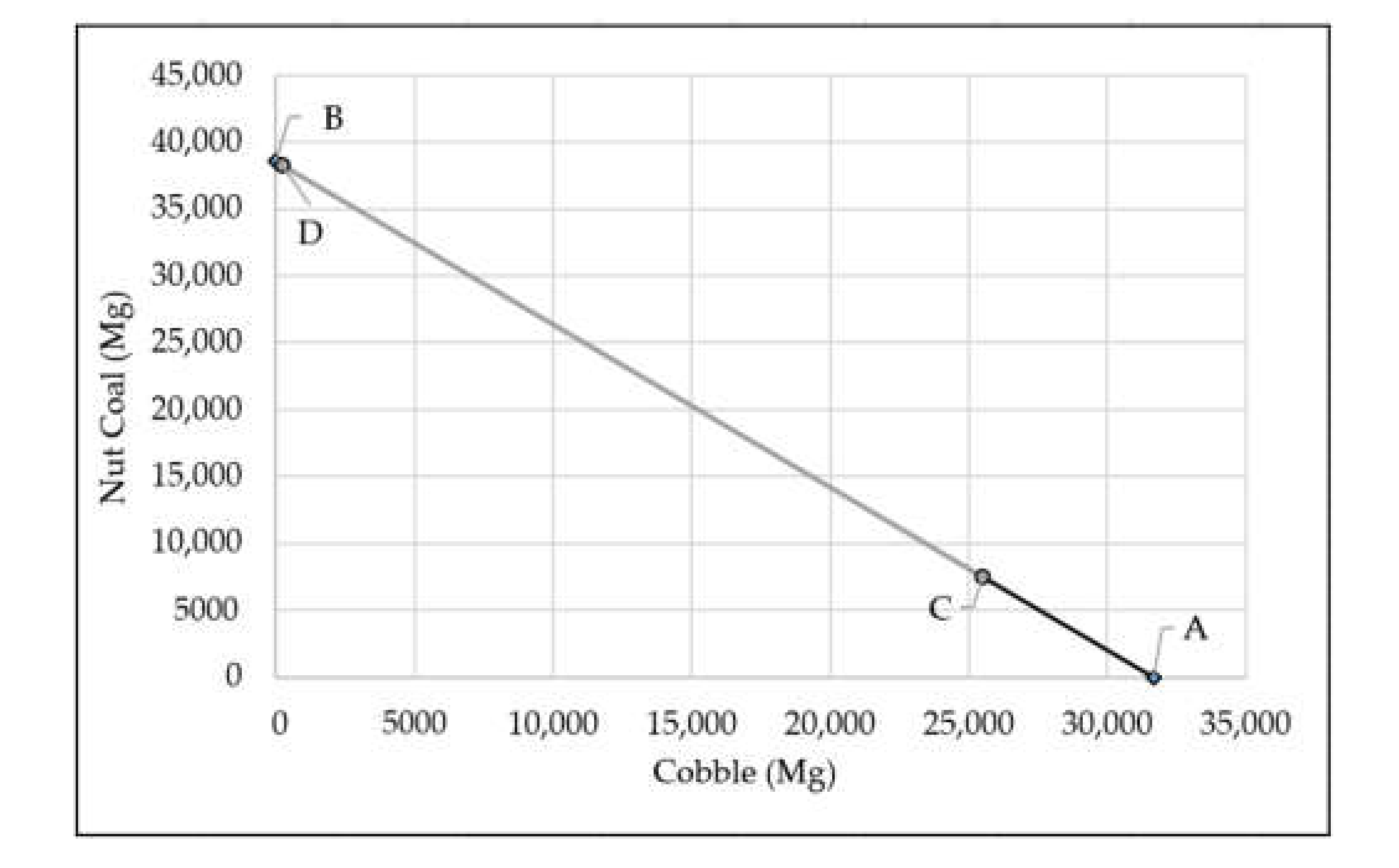
The threshold quantity of sales of the cobble sortiment for the analysed mine will be 31,680.86 Mg. On the other hand, producing and selling only nut coal, the break-even will be reached at 38,545.05 Mg, according to the calculations:

$$550\cdot 0+485\cdot P_N=11,563,515.55+185\cdot 0+185\cdot P_N$$

$$P_M=\frac{11,563,515.55}{300}=38,545,05(\mathrm{Mg})$$

Figure 1 presents a graphical solution for the analysed example. The determined boundary quantities of coal sortiments are marked in the diagram with letters A (for the cobble sortiment) and B (for the nut coal sortiment). These are points of intersection with the axes representing quantities of the analysed sortiments. Connecting points A and B leads to a segment AB which is a finite set of points (combinations of quantities of cobble and nut coal sortiments) fulfilling Equation (8). Each point of this segment guarantees finding it in the break-even.

However, this is not an acceptable solution due to the established production structure: 25,500 Mg of the cobble sortiment and 38,250 Mg of the nut coal sortiment. In this situation, an acceptable solution for the threshold quantities of the analysed sortiments will be a fragment of section AB, namely section CD, which is the result of the adopted production structure (Figure 1). In

Table 2. Example threshold quantities for cobble and nut coal assortments, sum of threshold quantities, and revenues.

Variants	Cobble	Nut Coal	Summarised Break-Even	Revenue	Revenue
	(Mg)	(Mg)	(Mg)	(PLN)	(€)
Variant 1	4000	33,678.39	37,678.39	18,534,016.8	(€4,100,446.19)
Variant 2	1000	37,328.39	38,328.39	18,654,266.8	(€4,127,050.80)
Variant 3	12,400	23,458.39	35,858.39	18,197,316.8	(€4,025,955.04)
Variant 4	11,132.92	25,000.00	36,132.92	18,248,105.6	(€4,037,191.50)
Variant 5	25,105.52	8000	33,105.52	17,688,037.1	(€3,913,282.54)
Variant 6	242.51	38,250	38,492.51	18,684,629.6	(€4,133,767.61)

, I have listed exemplary quantities of the cobble and nut coal sortiments, the sale of which also guarantees reaching the break-even (these are points lying on the CD segment). If we sum up the quantity of sales of sortiments (Table 2, column 4) for each variant, we would obtain the summarised break-even. As can be seen (Table 2) in each variant this total quantity is different. We do not obtain one specific value. Therefore, it is difficult to determine, having the information on actual sales at a given moment, whether the company is above the threshold (making profits), below the threshold (incurring losses), or perhaps at the threshold (zero profit).

In conclusion, the determination of threshold production (sales) quantities for individual products is a very complex issue, as there are an infinite number of combinations of their quantities that guarantee the company zero profit. Each method of determining a multi-assortment threshold proposed so far in the literature gives a single, unique solution. This is related to the way the authors choose to calculate the individual quantities of products from Equation (8). Each solution of the different methods is contained in a comprehensive set of solutions to Equation (8). For this reason, information about the specific threshold quantities that can be calculated by these methods is of little practical use and cannot be used as a basis for making any important production decisions. Their uselessness is due to the fact that actual sales of the product are very unlikely to approach the threshold quantities determined by any of these methods.

The methods presented in the literature also allow the calculation of the value of critical revenues (valuable threshold). Unfortunately, this is not one specific value, but again a finite, huge set. Columns 5 and 6 in Table 2 show the critical revenues for each variant of the threshold quantities of the cobble and nut coal sort (calculated by multiplying these quantities by the sales prices for the coal sortiment). Since there are an infinite number of variants of sales of particular sortiments and for each of them we obtain an equally numerous set of revenues, this information is not useful in practical application. Consequently, the methods on the basis of which we can calculate it are not useful either. It is worth noticing that the methods used so far make it possible to calculate only threshold quantities of sales of particular assortments and the value of revenue. So far, other than myself, no researcher has attempted to determine the percentage threshold. The percentage threshold provides one specific value characterising the condition of a given enterprise, as is discussed in Section 3.

As the number of produced assortments increases, the analysis becomes more complicated because of the dependencies between the individual assortments. It becomes even impossible to analyze the break-even.

3. Author’s Concept of Multi-Asset Break-Even Analysis

The method I have developed makes it possible to calculate the threshold percentage, which distinguishes it from the methods presented in the literature to date. The most important is that the percentage threshold is a single value, specific to a particular company. It provides information on the economic health of the company and, above all, enables quick determination of the financial situation of the company for the actual volume of sales at a given time.

I propose to determine its value according to the Equation (9):

$$PR(P)=\frac{Ks}{{\displaystyle \sum _{i=1}^n{P}_i\cdot (c_i-kj{z}_i)}}\cdot 100\%$$

(9)

PR(P) provides the following data: how much of the global gross margin goes to cover fixed costs. Topping up to 100% determines the achievable profit for the company. Its value, e.g., 60%, means that 60% of the global margin covers costs, and 40% brings the company a profit. The lower its value the better the financial health of the company.

I propose to use the following Equation (10) in order to determine the recognition of the quantitative threshold:

$$PR(I)=PR(P)\cdot P_m (\mathrm{Mg})$$

(10)

where:

• P_m—maximum production (sale) (Mg).

Whereas the threshold quantity of any assortment according to Equation (11) is:

$$P{p}_i=PR(P)\cdot P_{msi} (\mathrm{Mg})$$

(11)

where:

• P_ms—maximum output of the product (assortment) (Mg).

I propose that the valuable threshold be determined as the product of the percentage threshold and the maximum revenue in Equation (12):

$$PR(W)=PR(P)\cdot {\displaystyle \sum _{i=1}^n{P}_{msi}\cdot c_i} (\mathrm{PLN})$$

(12)

4. Results

The possibilities of practical use of the developed method will be demonstrated on the example of coal mines.

Table 3. Assumed value of production and economic indicators of mine “X” in a monthly take.

Coal Size Grade	Quantity	Unit Sale Price	Variable Cost	Total Cost
	(Mg)	(PLN/Mg)	(PLN/Mg)	(PLN)
Cobble	25,500	550 (€121.68)	185 (€40.93)	22,927,031.10
Nut Coal	38,250	485 (€107.30)	185 (€40.93)	(€5,072,352.01)
Fine Coal I	106,250	395 (€87.39)	185 (€40.93)	-
Fine Coal IIA	85,000	330 (€73.01)	185 (€40.93)	-
Fine Coal II	170,000	310 (€68.58)	185 (€40.93)	-
Total	425,000	-	-	-

shows the initial structure of the monthly production of mine “X”, as well as information on prices, variable unit costs of individual coal grades, and fixed costs. Whereas

Table 4. Assumed value of production and economic indicators of mine “Y” in a monthly take.

Coal Size Grade	Quantity	Unit Sale Price	Variable Cost	Total Cost
	(Mg)	(PLN/Mg)	(PLN/Mg)	(PLN)
Cobble	11,920	550 (€121.68)	197 (€43.58)	27,843,956.43
Nut Coal	23,833	485 (€107.30)	197 (€43.58)	(€6,160,167.35)
Fine Coal I	13,867	395 (€87.39)	197 (€43.58)	-
Fine Coal IIA	167,050	330 (€73.01)	197 (€43.58)	-

consists of analogous data for the mine “Y”.

The percentage threshold (Equation (9)) for mine “X” is:

$$PR(P)=\frac{22,927,031.10}{25,500\cdot (550-185)+38,250\cdot (485-185)+\dots +170,000\cdot (310-185)}\cdot 100=29.90(\%)$$

Whereas for mine “Y”:

$$PR(P)=\frac{27,843,956.43}{11,920\cdot (550-197)+23,833\cdot (485-197)+\dots +167,050\cdot (330-197)}\cdot 100=77.30(\%)$$

Mine “X” has a low break-even. Only about 30% of the gross margin covers fixed costs and 70% perhaps represents the maximum profit (achievable). It can be determined from Equation (13):

$$\mathrm{Profit}=(100\%-PR(P))\cdot {\displaystyle \sum _{i=1}^n{P}_{msi}\cdot (c_i-kj{z}_i)} (\mathrm{PLN})$$

(13)

Hence,

$$\mathrm{Profit}=(100\%-22.90\%)\cdot [25,500\cdot (550-185)+\dots +170,000\cdot (310-185)]=53,742,968.90\left(\mathrm{PLN}\right)(€11,890,037.37)$$

Hence, it can be considered that we are dealing with a rather high threshold in the case of Mine “Y” since as much as 77.30% of the gross margin is covered by fixed costs. The maximum achievable profit represents just under 23% from revenue less variable costs, as shown in Equation (13):

$$\mathrm{Profit}=(100\%-77.30\%)\cdot [11,920\cdot (550-197)+\dots +167,050\cdot (330-197)]=8,191,023.57\left(\mathrm{PLN}\right)(€1,812,173.36)$$

The proposed percentage threshold clearly defines the financial health of the company. In the case under review, the mine with the lower percentage threshold is in better financial condition. To confirm this, the profitability ratio (GPM) for both mines was calculated from Equation (14):

$$GPM=\frac{\mathrm{gross}\mathrm{profit}}{\mathrm{net}\hspace{0.33em}\mathrm{sales}}\cdot 100(\%)$$

(14)

For mine “X” it is:

$$GPM=\frac{53,742,968.90}{25,500\cdot 550+\dots 170,000\cdot 310}\cdot 100=34.61(\%)$$

And for mine “Y”:

$$GPM=\frac{8,191,023.57}{11,920\cdot 550+\dots 167,050\cdot 330}\cdot 100=10.41(\%)$$

Further analysis will be carried out for mine “X”. The threshold quantities of individual coal grades for mine “X” (calculated on the basis of Equation (11) are as follows:

$$P{p}_1=29.90\%\cdot 25,500=7625.40(\mathrm{Mg})\mathrm{for}\mathrm{cobble},$$

$$P{p}_2=29.90\%\cdot 38,250=11,438.10(\mathrm{Mg})\mathrm{for}\mathrm{nut}\mathrm{coal},$$

$$P{p}_1=29.90\%\cdot 25,500=7625.40(\mathrm{Mg})\mathrm{for}\mathrm{cobble},$$

$$P{p}_4=29.90\%\cdot 85,000=\mathrm{25,417.99}(\mathrm{Mg})\mathrm{for}\mathrm{fine}\mathrm{coal}\mathrm{IIA},$$

$$P{p}_5=29.90\%\cdot 170,000=50,835.99(\mathrm{Mg})\mathrm{for}\mathrm{fine}\mathrm{coal}\mathrm{II}.$$

Selling exactly these quantities will result in zero profit (reaching break-even). The results were intentionally left with decimal places, as rounding to whole tonnes will result in placing the mine in the profit zone (as shown below).

Do the calculated threshold quantities Pp₁–Pp₅ provide relevant information, which could be useful in practice? The answer is simple—unfortunately not. The probability of actual sales in threshold quantities Pp₁–Pp₅ is virtually zero. Only if actual sales of each coal grade were less than the threshold quantities could a mine be said to be below the threshold and making a loss. There is an infinitely large set of such solutions (threshold quantities) as follows from Equation (8).

Table 5. Summary of the threshold quantities of the individual coal grades, the total quantity threshold and the ad valorem threshold.

Cobble	Nut Coal	Fine Coal I	Fine Coal IIA	Fine Coal II	PR(I)	PR(W)	PR(W)
(Mg)	(Mg)	(Mg)	(Mg)	(Mg)	(Mg)	(PLN)	(€)
7625.40	11,438.10	31,772.49	25,417.99	50,835.99	127,089.97	46,438,675.65	10,274,043.29
0.00	0.00	48,462.05	0.00	102,000	150,462.05	50,762,510.88	11,230,644.00
9500	5360	61,578.72	21,000	15,000	112,438.72	43,728,194.22	9,674,379.25
12,200	14,000	33,221.58	43,000	8500	110,921.58	43,447,522.79	9,612,283.80
2000	0.00	105,700.15	0.00	0.00	107,700.15	42,851,558.50	9,480,433.30
15,000	34,256.77	0.00	15,000	40,000	104,256.77	42,214,533.62	9,339,498.59

summarises six example combinations of sales of individual coal grades, the sale of which in such quantities also guarantees that the mine reaches break-even.

Total volume break-even (calculated from Equation (10)):

$$PR(I)={\displaystyle \sum _{i=1}^{n}P{p}_i}=127,089.97(\mathrm{Mg})$$

also makes up the set of finitely many admissible solutions (column 6 of Table 5, (PR(I)). As can be seen, each solution gives a different value for the aggregate quantitative threshold. It is not one specific value, so we are not able to say whether actual sales are profitable or loss-making.

The situation is analogous with the valuable threshold (column 7 of Table 5, PR(W))—calculated from Equation (12):

$$\begin{array}{c}PR(W)=29.90\%\cdot \left[7625.40\cdot 550+11,438.10\cdot 485+31,772.49\cdot 395+25,417.99\cdot 330+50,835.99\cdot 310\right]\\ PR(W)=46,438,675.65(\mathrm{PLN})(€10,274,043.29)\end{array}$$

There are as many solutions as there are values for the valuable threshold. Unfortunately, this is not one particular value, but again, a finitely numerous set. Therefore, information on the value of income is also not useful in practice.

Let us consider different hypothetical variants for the sale of coal grades of mine “X” (

Table 6. Variants of sales of size grades of coal of mine "X" on a monthly basis (Mg).

Sales Scenario	Cobble	Nut Coal	Fine Coal I	Fine Coal IIA	Fine Coal II
	(Mg)	(Mg)	(Mg)	(Mg)	(Mg)
Threshold quantity	7625.40	11,438.10	31,772.49	25,417.99	50,835.99
I	7626	11,439.00	31,773.00	25,418.00	50,836.00
II	7600	11,440.00	31,780.00	25,418.00	50,870.00
III	9500	5360	32,000.00	21,000.00	64,000.00
IV	5000	5000	30,000.00	20,000.00	90,000.00
V	0.00	0.00	48,462.05	0.00	102,000.00

).

The presented variants (combinations) of sales I–V do not explicitly state whether mine “X” is in the profit, loss, or zero zone. To determine this, the proposed percentage threshold, i.e., knowledge of one characteristic quantity, will be useful. First, the proposed Equation (15) is used by calculating the current sales ratio:

$$WAS=\frac{{\displaystyle \sum _{i=1}^n{P}_i\cdot (c_i-kj{z}_i)}}{{\displaystyle \sum _{i=1}^n{P}_{mi}\cdot (c_i-kj{z}_i)}}\cdot 100(\%)$$

(15)

Based on Equation (15), the percentage share of the currently realised gross margin in relation to the global margin (achievable with total sales of all products) is determined. The calculated value of current sales ratio (WAS) should be compared with the proposed percentage threshold. We immediately receive an unambiguous answer:

• WAS < PR(P)—the company is incurring losses,
• WAS = PR(P)—the company has met the break-even (profit is 0),
• WAS > PR(P)—the company is making profit.

For variant I (Table 6), the WAS value (according to Equation (15)) is:

$$WAS=\frac{7626\cdot (550-185)+11,439\cdot (485-185)+\dots +50,836\cdot (310-185)}{25,500\cdot (550-185)+38,250\cdot (485-185)+\dots +170,000\cdot (310-185)}\cdot 100=29.904(\%)$$

WAS > PR(P) so selling in such quantities makes a profit for the mine.

To assess what financial result (profit/loss) a mine achieves for a given volume of sales, it should be calculated according to Equation (16):

$$WF=(WAS-PRP)\cdot {\displaystyle \sum _{i=1}^n{P}_{msi}\cdot (c_i-kj{z}_i)} (\mathrm{PLN})$$

(16)

For variant I, the following financial result is obtained after substituting the data (according to Equation (16)):

$$\begin{array}{c}WF=(29.904-29.903)\cdot [25,500\cdot (550-185)+38,250\cdot (485-185)+\dots +170,000\cdot (310-185)]\\ WF=598.90 \left(\mathrm{PLN}\right)(€132.50)\end{array}$$

When analyzing variant II, it should be stated that the WAS value is (according to Equation (15)):

$$WAS=\frac{7600\cdot (550-185)+11,440\cdot (485-185)+\dots +50,870\cdot (310-185)}{25,500\cdot (550-185)+38,250\cdot (485-185)+\dots +170,000\cdot (310-185)}\cdot 100=29.899(\%)$$

WAS < PR(P) so selling in such quantities makes the mine a loss (Equation (16)):

$$\begin{array}{c}WF=(29.899-29.903)\cdot [25,500\cdot (550-185)+38,250\cdot (485-185)+\dots +170,000\cdot (310-185)]\\ WF=-2,871.10\left(\mathrm{PLN}\right)(-€635.20)\end{array}$$

In variant III, the WAS value is (Equation (15)):

$$WAS=\frac{9500\cdot (550-185)+5360\cdot (485-185)+\dots +64,000\cdot (310-185)}{25,500\cdot (550-185)+38,250\cdot (485-185)+\dots +170,000\cdot (310-185)}\cdot 100=29.791(\%)$$

WAS < PR(P) so selling in such quantities also makes the mine a loss (Equation (16)):

$$\begin{array}{c}WF=(29.791-29.903)\cdot [25,500\cdot (550-185)+38,250\cdot (485-185)+\dots +170,000\cdot (310-185)]\\ WF=-86,531.10 \left(\mathrm{PLN}\right)(-€19,144.05)\end{array}$$

For variant IV, the WAS value is:

$$WAS=\frac{5000\cdot (550-185)+5000\cdot (485-185)+\dots +90,000\cdot (310-185)}{25,500\cdot (550-185)+38,250\cdot (485-185)+\dots +170,000\cdot (310-185)}\cdot 100=31.009(\%)$$

WAS > PR(P) so selling in such quantities makes a profit for the mine (according to Equation (16)):

$$\begin{array}{c}WF=(31.009-29.903)\cdot [25,500\cdot (550-185)+38,250\cdot (485-185)+\dots +170,000\cdot (310-185)]\\ WF=847,968.89 (\mathrm{PLN}) (€187,603.74)\end{array}$$

In variant V, the WAS value is:

$$\begin{array}{c}WAS=\frac{0\cdot (550-185)+0\cdot (485-185)+48,462.05\cdot (395-185)+0\cdot (330-185)+120,000\cdot (310-185)}{25,500\cdot (550-185)+38,250\cdot (485-185)+\dots +170,000\cdot (310-185)}\cdot 100\\ WAS=29.903(\%)\end{array}$$

WAS = PR(P) so selling in such quantities makes the mine zero profit. The mine is at the break-even.

5. Discussion and Conclusions

As can be observed, the proposed WAS indicator is an important element of the multi-asset threshold analysis, which allows a quick assessment of the financial result on the currently realised sales volume by comparing WAS with PR(P). The practical usefulness increases when analysing numerous variants of mine production scenarios (the author analysed scenarios of 1000 and 10,000). The methods of multi-asset break-even analysis available in the literature, based solely on the quantitative and valuable recognition, do not meet the practical usefulness.

The author hopes that the examples cited have helped the reader to understand the issue of the multi-assortment threshold and prove the thesis that the proposed method is of practical use, especially that the percentage threshold is relevant to solving this issue.

The method I propose for calculating and analysing the break-even in multi-assortment production is an effective tool for supporting rational production decisions. Its usefulness lies in its simplicity and the possibility of obtaining an unambiguous result. It has been positively verified during my research for its practical applicability in the mining industry.

The sole knowledge of the quantitative threshold and the aggregate ad valorem threshold does not make it possible to state unequivocally in what position (in relation to the threshold level) the mine is. Only the proposed percentage threshold creates such clarity.

The percentage threshold I developed makes it possible to assess the company’s economic health, analyse its dynamics, and allow comparisons with other mines in the industry.

Conditions, both internal and external, force a verification of the set objectives and significantly affect the sales level of individual assortments, their share in the production structure, and the sales price. All these considerations necessitate the importance of determining the percentage of break-even.