Article

Optimal D-STATCOM Placement Tool for Low Voltage Grids

by
Gregorio Fernández
1,*,
Alejandro Martínez
1,
Noemí Galán
1,
Javier Ballestín-Fuertes
1,
Jesús Muñoz-Cruzado-Alba
1,
Pablo López
2,
Simon Stukelj
3,
Eleni Daridou
4,
Alessio Rezzonico
5 and
Dimosthenis Ioannidis
6
1
Fundacion CIRCE, Parque Empresarial Dinamiza, Avenida Ranillas 3-D, 1st Floor, 50018 Zaragoza, Spain
2
Grupo Cuerva, C/Santa Lucia, 1 K. Churriana de la Vega, 18194 Granada, Spain
3
E.ON Energilösningar AB, 205 09 Malmö, Sweden
4
HEDNO, 47 Syngrou Av., 117 42 Athens, Greece
5
AEM, Via Lisano 3, 6900 Massagno, Switzerland
6
Centre for Research and Technology-Hellas, Information Technologies Institute, 57001 Thessaloniki, Greece
*
Author to whom correspondence should be addressed.
Energies 2021, 14(14), 4212; https://doi.org/10.3390/en14144212
Submission received: 4 June 2021 / Revised: 1 July 2021 / Accepted: 2 July 2021 / Published: 12 July 2021
(This article belongs to the Special Issue Control and Optimization of Renewable Energy Systems)

Abstract

:
In low-voltage grids with a wide spread of domestic and/or small commercial consumers, mostly single-phase, problems can appear due to unbalanced power consumption between the different phases. These problems are mainly caused due to voltage unbalances between phases and the increase in distribution losses. This phenomenon occurs more frequently at the end of highly radial grids and can be stressed by the installation of renewable generators next to the consumers. Amongst the various techniques that have been proposed to solve this problem, this article explores the use of a D-STATCOM, presenting and testing a new method for the optimal location of this type of D-FACT. The developed method starts from a detailed analysis of the existing voltage unbalances in a distribution network and identifies the optimal location of the D-STATCOM (i.e., the one that reduces these unbalances while reducing energy losses). The developed method has been successfully tested for one year at four real European locations with different characteristics and different kinds of users.

1. Introduction

Classical electric power generation technologies based on thermal cycles use gas, oil, or coal as the main source of energy. For years, it has been proven that the use of these fossil fuels is one of the main causes of climate change, which has resulted, among other consequences, into global warming, which is expected to reach a 1.5 degrees Celsius temperature rise by 2030 [1]. An increasing social awareness on climate change [2] and new regulations [3,4], coupled with a great technology progress and price reductions, have placed renewable energy as one of the main solutions to environmental problems.
Despite their advantages, high penetrations of renewable energies can generate problems due to their intermittent, seasonal, and uncontrollable nature. Transmission system operators (TSOs) have been facing these problems for years and distribution system operators (DSOs) are beginning to observe this due to the high diffusion of distributed generation. These new problems are forcing DSOs and TSOs around the world to develop new operation and maintenance techniques and structures in their systems [5].
Distributed energy resources (DERs) consist of small/medium-scale resources that are connected to the distribution grid at low voltage (LV) levels, near the end users [6,7], and will play a key role in the energy sector in the near future. These increased penetration levels of DER transform distribution grids into active systems. The new network structure generates bi-directional power flows between the transmission and distribution systems. This represents an advantage since distribution grids will export energy when local generation exceeds consumption, and consumers can now become an active part of the network, benefiting from generation excesses by injecting it into the network [7].
On the other hand, due to the variability of distributed energy generation such as wind or PV systems and long lines, problems such as the following become common in dispersed urban and rural LV networks [8]:
Voltage rise. Low penetration of PV improves voltage profile and reduces losses in the system [9], but high penetration can cause overvoltage problems at peak PV generation hours when there is low demand in the LV network [10,11]. This problem is significantly lower in areas with a combination of residential and commercial consumers [12], but may be of concern in purely residential areas.
Grid congestion. A high penetration of DERs can cause power swing problems. If the penetration is too high (compared to the demand), reverse power flow could appear, affecting grid components or electrical protections. References [13,14] highlight congestion problems in distribution grids.
Harmonics. Considering the high penetration of DERs, it is likely that the system will behave in a non-linear way. This could lead to harmonic problems that will decrease the quality of the power delivered to the consumers. The limits of total harmonic distortion (THD) and total demand distortion (TDD) are only violated at relatively high PV penetration. In [15], in a LV distribution grid with high PV penetration (60% with respect to the transformer rating), the THD is over the 5% limit. Furthermore, it has been observed that the power electronics of renewable facilities generate an electromagnetic noise that could reduce quality of the PLC (power-line communication) communications. Although it is not very common nowadays, a high penetration of power electronics equipment in the consumers could make this effect more common.
Voltage unbalances. The LV distribution grid runs on three phases, but many consumers are single-phase connected. Moreover, high penetration levels of PVs result in voltage unbalances and neutral currents, and these violations of balance limits are strongly related to the location and the phase to which the PV systems and consumption points are connected [16]. At the beginning of a distribution feeder, voltage unbalance is low, and can be kept within the standard limits regardless of the number, location, and rating of installed rooftop PVs. However, unbalance might increase at the end of the feeder above the standard limits [17]. In [18,19], the impact of residential PV installations on voltage unbalance was studied, showing that the unbalance can increase from 1% to 3%. Voltage unbalance caused by PV may even cause disconnection of the system due to unintentional impact of the voltage regulation scheme [20]. This produces an unbalance in the other phases that leads to increased currents and losses.
There are several solutions to address the aforementioned problems of DERs:
  • Grid reinforcing is an alternative to the congestion problems generated by the high penetration of DERs. This reinforcement is linked to technical and economic regulations [21,22].
  • To solve grid congestion problems, active power limits for demand or generation (depending on the origin of the congestion) can be set. Other congestion management methods are discussed in [23].
  • To avoid introducing harmonics into the network, a good solution is the installation of conventional active power line conditioners (APLCs) and/or active power filters (APFs) to have a high harmonic filtering capability [24].
  • The connection of PV generators as three-phase systems is a good proposal to reduce losses and unbalances. Conversely, this would not be feasible because most prosumers have single-phase connection to the network [25].
  • Storing energy near prosumers is another extensively studied option, which can adapt generation to consumption patterns, reducing reverse power flows and voltage increases. The cost of storage technologies should be reduced to make this solution economically viable [26].
  • Support from prosumers to solve these issues is currently increasing. This is done through demand management, from which both prosumers and DSOs benefit [27].
  • Reactive power control of PV inverters and wind generators dependent on the grid voltage or generated active power are solutions for the efficient use of wind and PV and enable high penetration revivals systems in distribution grids [28,29].
A recent study [30] described the methodology applied in a low voltage network in southern Spain to calculate the optimal photovoltaic hosting capacity that minimizes system losses. This paper is more influential compared to other similar studies, since it uses real data from smart meters and other data provided by the electrical distributor. The report also evaluated management techniques for solar PV inverters and their effect on the hosting capacity. As a result, as distributed PV generation increases, more voltage deviation problems occur in the network. Constant power reactive control or power factor (PF) setpoints had the best results when solving these problems.
Aside from the previous points, the use of static VAR compensator (SVC) or set voltage regulators (SVRs) is proposed to solve voltage deviations [31] and unbalances [32,33,34,35,36]. In keeping with the use of flexible AC transmission systems (FACTS), the use of a distribution static synchronous compensator (D-STATCOM) is proposed and addressed in the present document. The use of D-STATCOM systems in the distribution networks in low voltage levels can solve the problems caused by the high penetration of DER due to its ability to control frequency, amplitude, and phase of the output voltage. Compared to the passive compensators, power electronics-based active compensators exhibit better and more reliable results in the neutral current compensation process [16].
As already mentioned, voltage unbalances are local in nature and can vary in value geographically and temporally. In addition, they are strongly influenced by the characteristics of the consumption and generation points in the area, being normally higher in areas with a wide proportion of single-phase customers and at points far from the secondary transformer substation. These characteristics mean that finding the best location for the D-STATCOM is fundamental, which is the reason why there is so much literature on the subject. In fact, an incorrect placement and management of a D-STATCOM would not only limit its benefits, but may even worsen or jeopardize the proper operation of the network [37].
The most common objective functions found in the related literature are [38]:
  • Power loss mitigation.
  • Voltage profile improvement.
  • Cost reduction.
  • Voltage stability improvement.
  • Reliability improvement.
  • Load balance improvement.
  • THD reduction.
The most common restrictions are [31]:
  • Power balance.
  • Voltage deviation limits.
  • D-STATCOM capacity limits.
  • Reactive power compensation.
  • Current limit.
  • Cost limitations.
There are several classifications for the optimal D-STATCOMs’ placement and sizing methods. The authors in [38] describe the following:
  • Analytical methods that propose optimal solutions without considering nonlinearities and complexities in the problems to reduce computational effort.
  • Artificial neural network methods that can deal with non-linear systems and more complex problems.
  • Metaheuristic methods (the most spread ones). These algorithms are stochastic methodologies and population-based ones, which are generally efficient, but can propose local minimums (or maximums) as the optimal solution.
  • Sensitivity approaches that allocate the D-STATCOM according to the value of an index. The most common ones are voltage sensitivity index (VSI) and power loss index (PLI), calculated for the possible locations of the evaluated grid. In these methods, the D-STATCOM is not emulated and only the index is calculated, and the location with the optimal index is chosen to fit the D-STATCOM.
  • Combination of sensitivity approaches and metaheuristic methods.
For example, [39] proposed an analytical method to search along all the nodes of the grid to find the location, and the D-STATCOM power that jointly minimizes energy losses and voltage variations.
A number of authors have proposed the use of nature-inspired metaheuristic techniques to find the optimal location and dimensioning of one or more D-STATCOMs. For example, [40,41] proposed the use of particle swarm optimization (PSO) methodology to find the terminal in which the D-STATCOM would result in minimum losses in the network. The PSO is a numerical optimization method used to solve many tasks in the field of energy engineering, combining a very simple implementation and a very good convergence. The method simulates a multi-agent system, where particle agents move toward optimal solutions while exchanging information with neighbors. In the swarm method, each potential solution is represented by a point in the spatial search called the particle [42]. The algorithm of the PSO represents an iterative method that continues until the stop criterion is met.
Other metaheuristic approaches proposed for the optimal placement of a D-STATCOM are the harmony search method (HSM) [37] or ant colony optimization (ACO). In [43], the ACO algorithm was used to calculate the optimal placement, size, and amount of D-STATCOMs and incorporated the cost of the devices within the optimization process.
As an example, [44,45,46] proposed the use of a sensitivity approach by calculating the VSI for all nodes of a grid and choosing the location of the D-STATCOM as the one with the highest voltage sensitivity index value. Other works delve into the index approach: [47] proposed variations on the VSI calculation to optimally locate and size D-STATCOMs. Reference [48] used the sensitivity approach through the VSI to increase reactive loading capability and to improve voltage profiles; in [49], they presented a probabilistic technique for optimal allocation of the D-STATCOM, considering the correlation between uncertain variables and improving the expected voltage deviation index (VDI) and decreasing the expected installation cost for D-STATCOM in radial/mesh distribution networks.
The authors in [50] proposed a combination of sensitivity approaches and metaheuristic methods such as VSI and the grey wolf optimizer (GWO) metaheuristic algorithm for optimal placement and sizing of a solar PV facility and a D-STATCOM. The study in [51] presented a new lightning search algorithm (LSA) combined with the VSI index. The studies in [52,53] proposed a genetic algorithm (GA) and PSI and VSI indexes to optimally locate a D-STATCOM.
In this context, the contribution of the present paper can be summarized as:
  • The proposal of a novel methodology to find the optimal location of a single fixed power D-STATCOM for distribution loss reduction through voltage unbalance compensation. None of the reviewed documents deal with this issue of voltage unbalance.
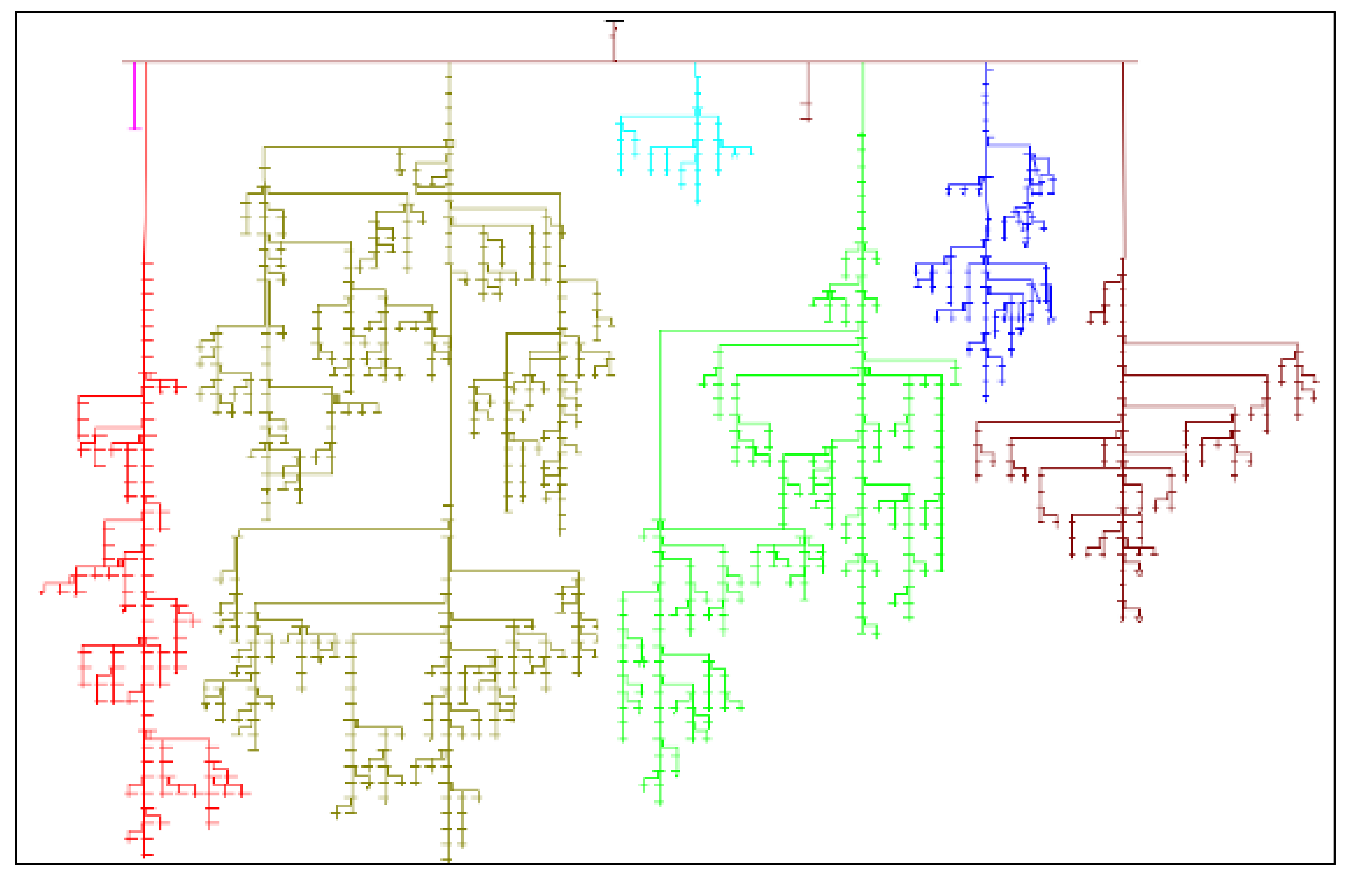
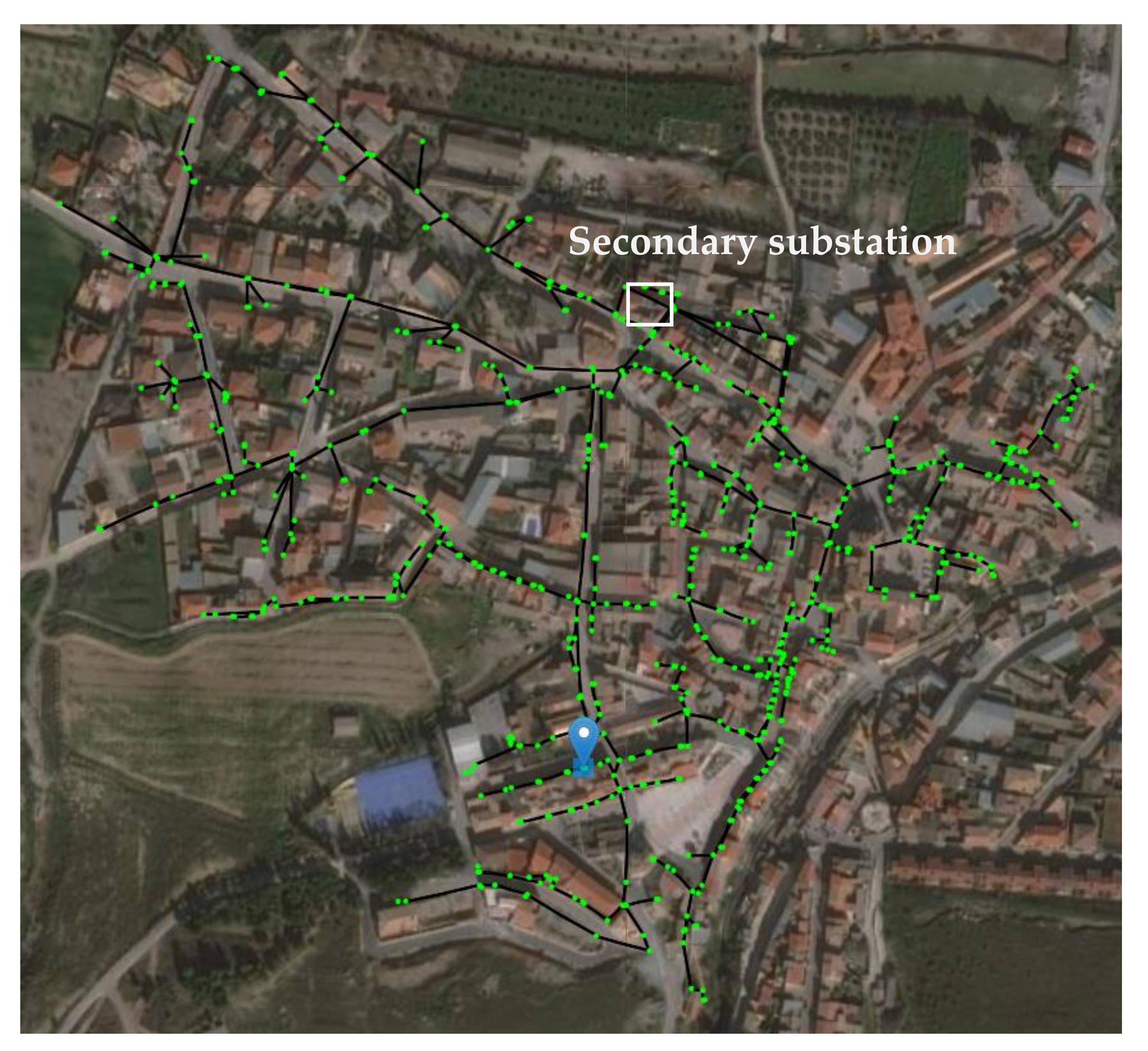
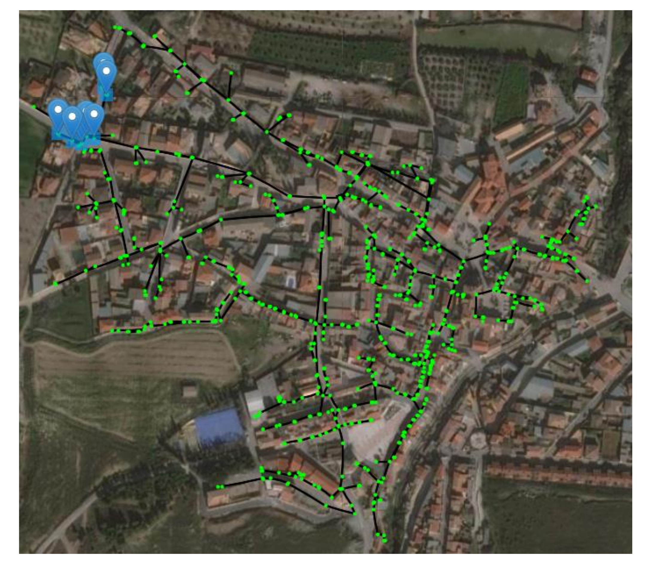
  • The proposed methodology was tested using the data obtained from four real grids during a whole year. These were located in four different European countries and have different characteristics and topologies: urban, rural, residential, etc.
The proposed method works in two steps: first, to identify the locations most likely to host the device, and a second in which the effect of a single D-STACOM of a predefined power is emulated at these points and their neighbourhood. The initial search field was determined by locating the nodes of the network with the most voltage unbalances. The search process in neighboring nodes to those initially proposed has been proven to be simple and effective. The proposed method can be considered as a combination of sensitivity approaches and metaheuristics methods: the voltage unbalance would be the sensitivity index that provides the initial search space, and the proposed neighborhood search is a variation of the “variable neighborhood search” method [54]. Other documents that propose combinations of sensitivity approaches and metaheuristics methods focus on voltage sensitivity and power loss indices. As far as the authors are aware, this is the first paper focusing on reducing voltage unbalances and the energy losses associated with this phenomenon.
In Section 2, the proposed methodology is described. In Section 3, the results of applying this tool to four real networks are presented. In the Discussion and Conclusions sections, the results obtained by the proposed methodology are commented and finally, the main conclusions obtained through this work are highlighted and future lines of development are proposed.

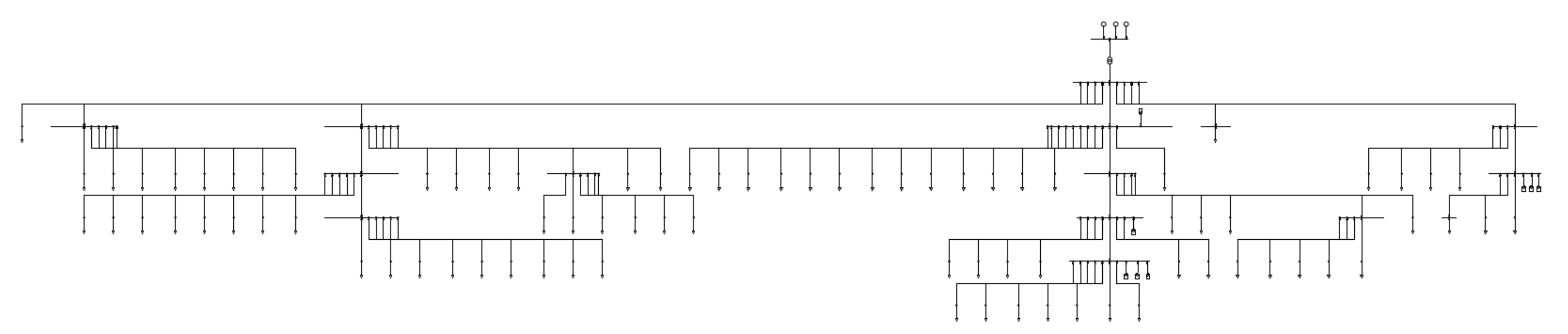
2. Materials and Methods

The objective of this optimal D-STATCOM placement tool was to find—in low voltage distribution grids—the node where a D-STATCOM with predefined characteristic minimizes distribution energy losses by balancing phases and compensating reactive power consumption.
To develop, test, and debug this tool, real data from different distributors have been used. The selected demonstrators are listed below (complete descriptions of these networks can be seen in Appendix A):
-
Southern Europe rural grid.
-
Northern Europe urban-residential grid.
-
Central Europe rural-residential grid.
-
Southern Europe urban grid.
For the simulations, the following inputs were available:
-
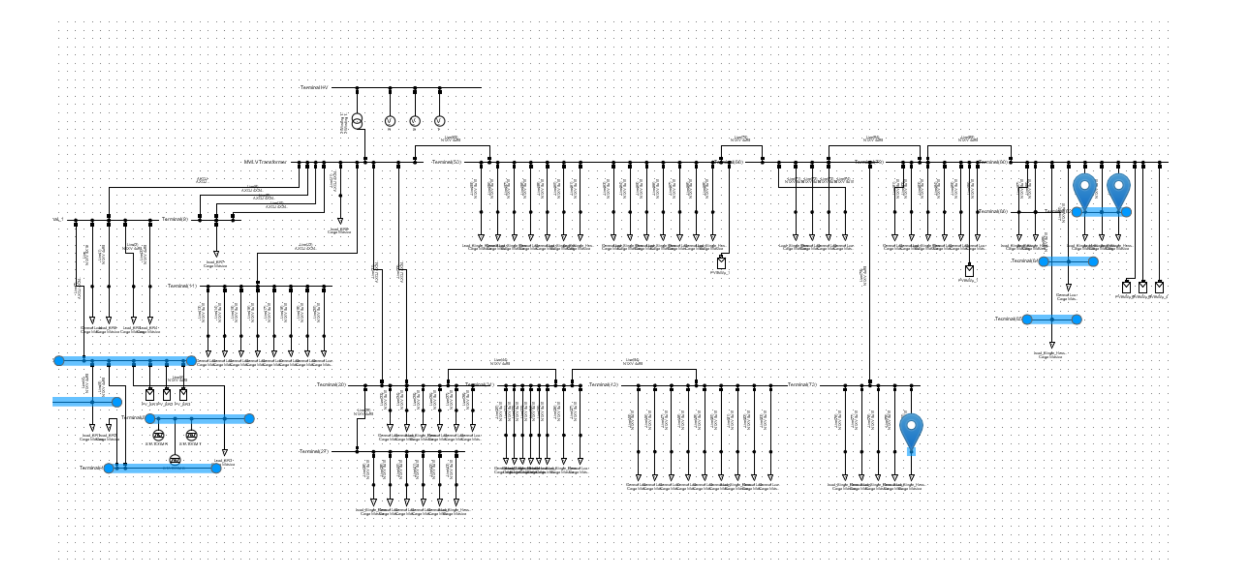
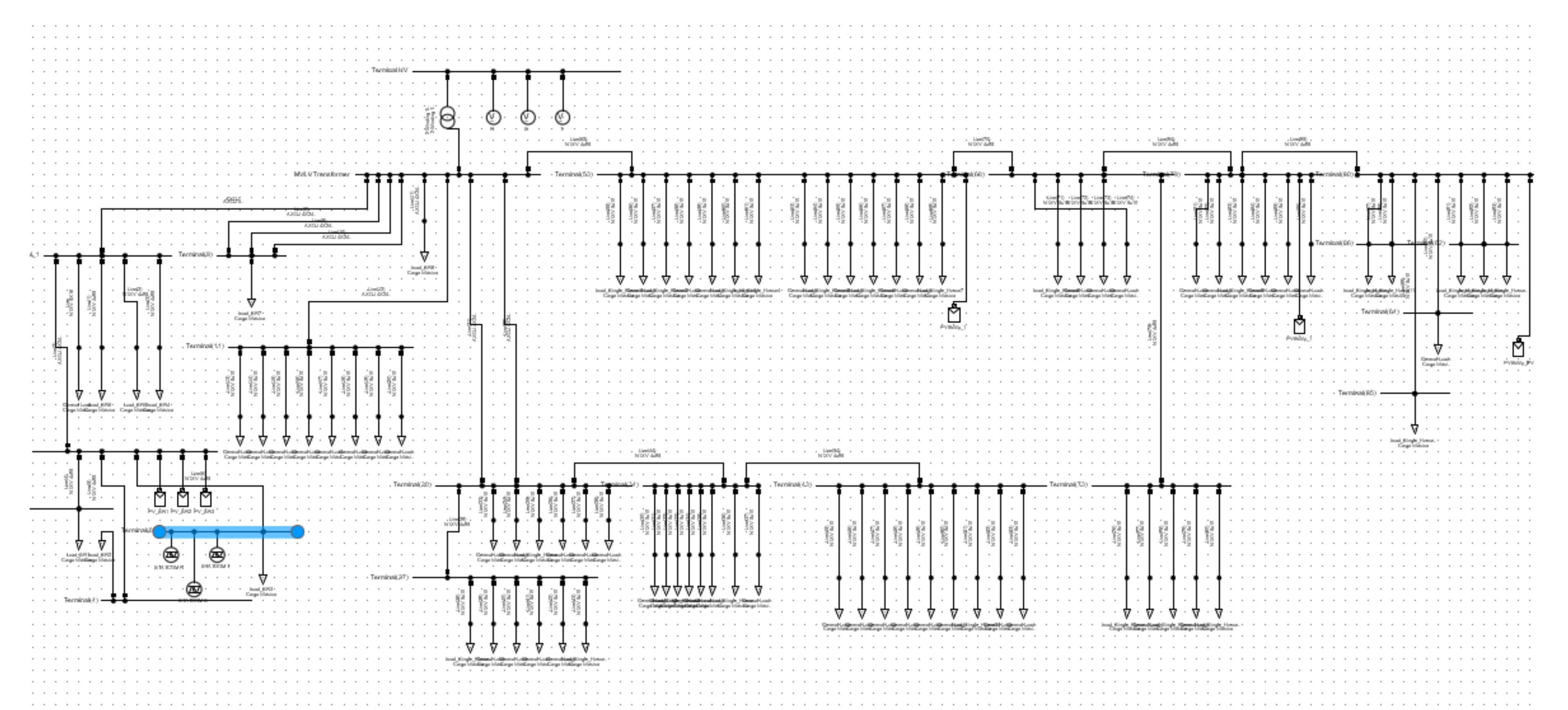
Network model in PowerFactory DIgSILENT [55].
-
Consumption data from smart meters of the customers.
-
Historical data of voltage in the secondary substation.
-
Solar irradiation and installed power of solar photovoltaic generation facilities.
-
The methodology to detect unbalances in the network and to correct them by using a D-STATCOM installed in the optimal location is explained in detail in the next sections.

2.1. Energy Loss Minimization

The objective of this optimization process is minimizing distribution energy losses by minimizing the sum of the losses generated in all sections of the network analyzed and over the period studied. The objective function is Equation (1):
min :   n , t I n , t 2 · R n , t ,
where n is the number of lines in which losses are generated and t is the number of time steps in which the period under analysis is divided. The constraints are those of a power flow:
  • Line currents and nodes voltages.
  • Power balance.
  • D-STATCOM power limits and operation characteristics.
A second group of constraints were the ones that describe the node characteristics: the nodes able to host the D-STATCOM must be underground and three-phase.

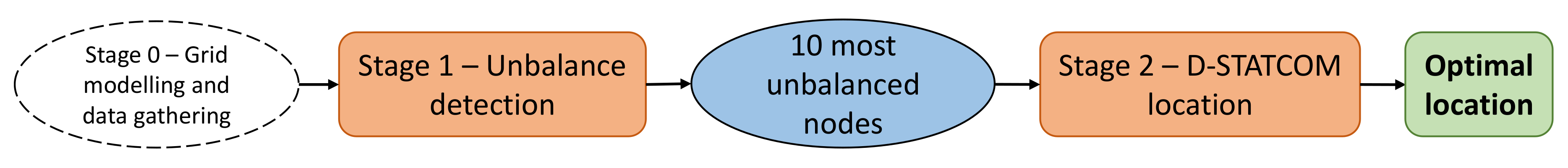
2.2. Algorithm Description

The proposed methodology operates in two steps or stages (see Figure 1):
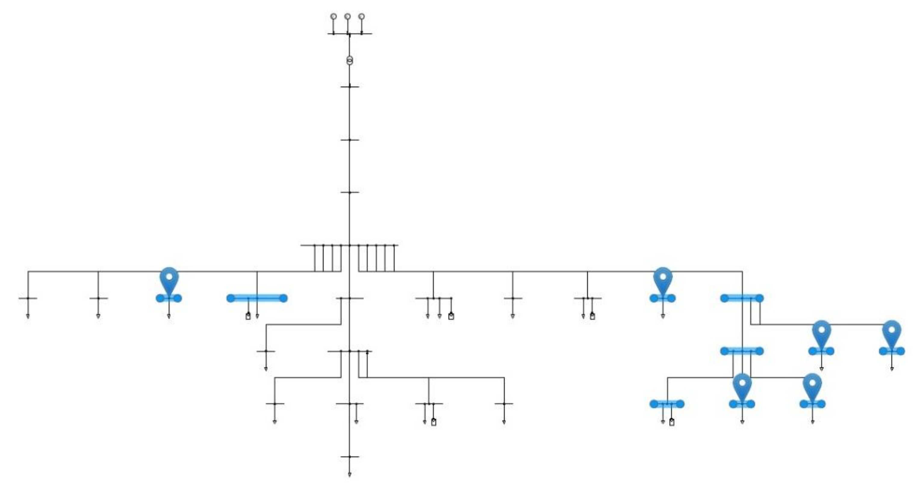
  • Unbalance detection stage: it detects nodes in which unbalances are higher than the established limit.
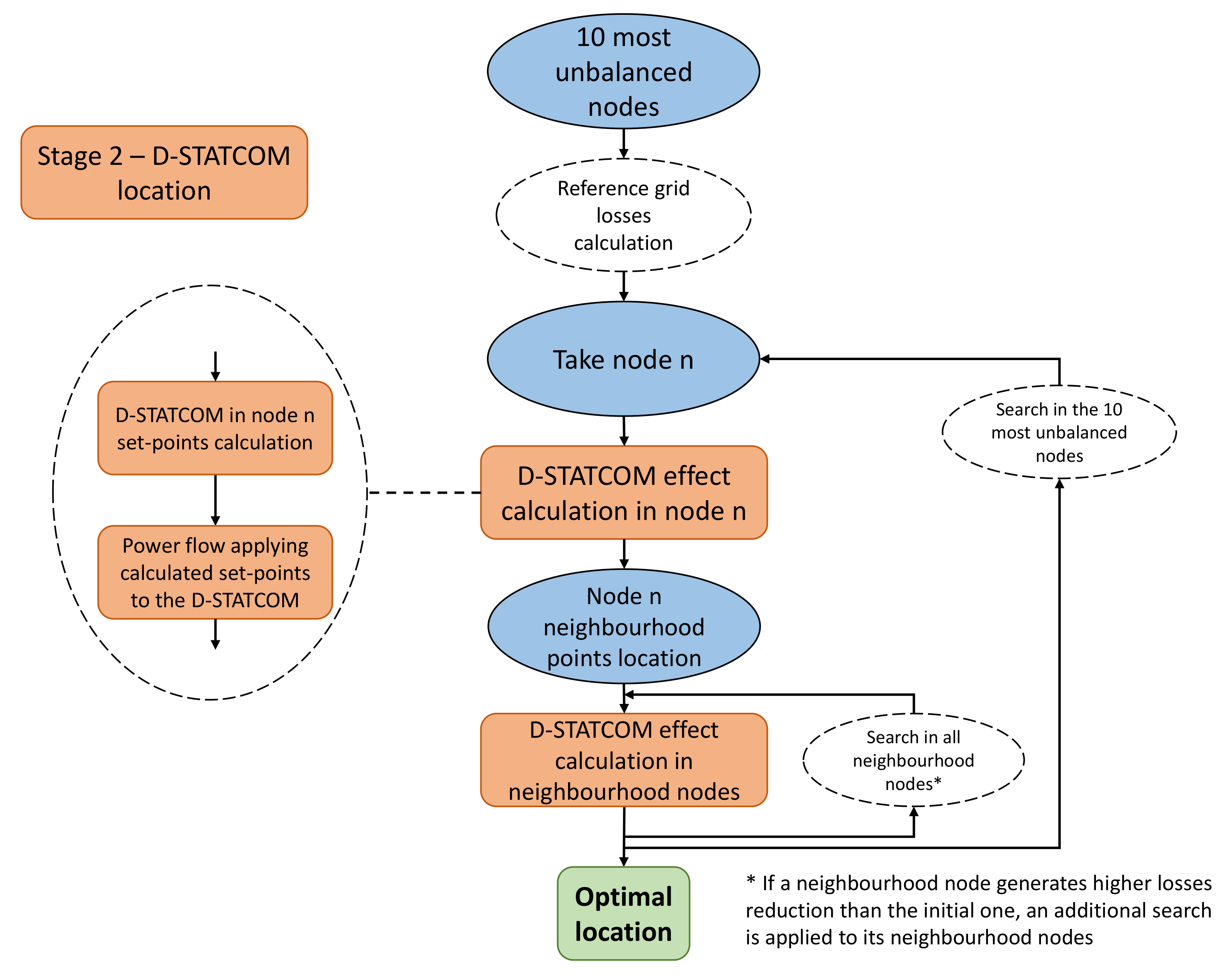
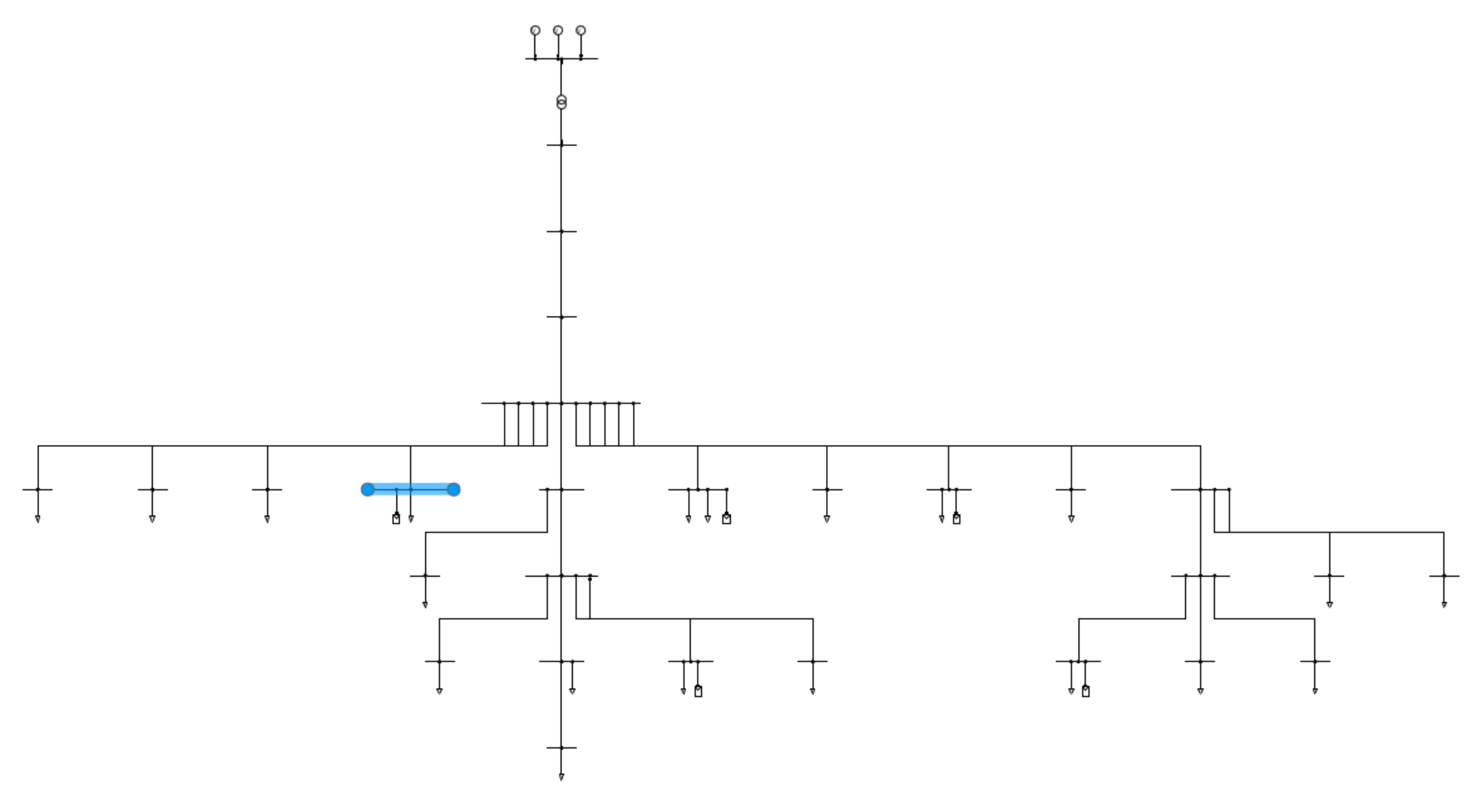
  • D-STATCOM location stage: it uses the points of major unbalance provided by the previous step to emulate the D-STATCOM behavior and to find its optimal location. In this stage, the proposed methodology analyzes, in an iterative process, the list of 10 nodes with higher voltage unbalance and the neighborhood points.

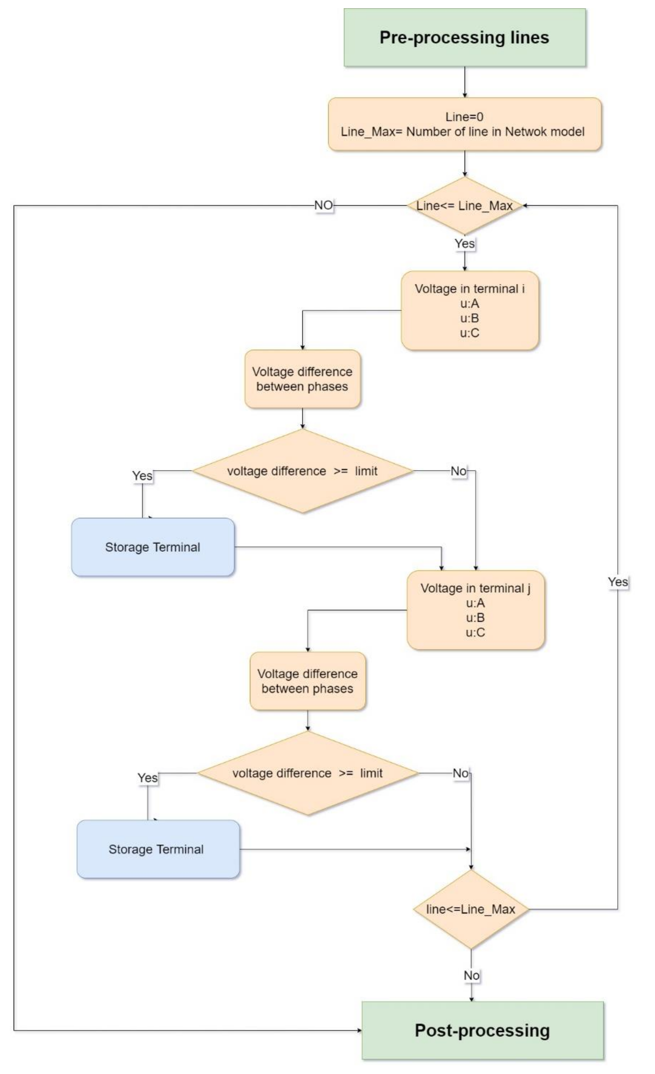
2.2.1. Unbalance Detection Stage

The “unbalance detection phase” detects the unbalances that occur in the network due to:
  • Three-phase consumers not consuming in a balanced way.
  • Single-phase consumers.
In the first step, the conditions to be satisfied by the connection points (“pre-processing lines”) for the possible installation of D-STATCOM are determined. Several conditions have been set:
  • The line must be three-phase. This refers to the fact that D-STATCOM compensates the three phases so the line should be three-phase.
  • The lines should be in service.
Quasi-dynamic analysis is used to calculate the hourly load flow, and then the unbalances between phases are extracted from it. The quasi-dynamic analysis granularity and duration depend on the available data. In the four scenarios tested in this paper, the work was performed in hourly intervals for one year.
After the load flow calculation, the unbalance of voltage between phases is analyzed and, if a terminal has an unbalance higher than a pre-established threshold, it is added to the list of nodes that could host the D-STATCOM. Figure 2 shows the flowchart of the unbalance detection stage.
For each hour of the analyzed period, the process shown in Figure 2 was executed, in which the existing unbalances between the three phases (A, B, C) at the initial (i) and final (j) nodes were calculated. Only the unbalances between phases (Uab, Uac, Ubc) that exceeded the maximum limit were stored and considered as candidates to host the D-STATCOM. This limit (adaptable to the regulations applicable to the analyzed network) was set at 2%, as per the EN50160 standard [56].
In post-processing, the terminals were sorted based on the following priorities:
  • Number of unbalances occurrences in the period studied.
  • Average unbalance between phases AB, AC, and BC in the period studied.
  • Maximum unbalance between phases AB, AC, and BC in the period studied.
This order is logical because the maximum power of the D-STATCOM is fixed at 30 kVA and selecting a location to solve high but infrequent unbalances can make it underused.
Therefore, the nodes at the top of the list as per the sorting order explained above are the most appropriate to host the D-STATCOM and are used in the next phase of the methodology. In this case, 10 nodes were chosen as the starting point, although this number could be modified depending on factors such as the size of the network or the ratio of single-phase or unbalanced consumers with respect to the total consumers.

2.2.2. D-STATCOM Location Stage

The aim of the “D-STATCOM location” stage is to find the location of the D-STATCOM that minimizes distribution energy losses, see Figure 3. For this purpose, the ten candidate locations obtained from the “unbalance detection” stage were taken as a starting point. In a second phase of this process, the initial search space is extended by adding neighboring nodes.
In a process similar to the methodologies based on PSO techniques [57], once the effect of the D-STATCOM has been calculated at one point, its potential effect on the neighboring nodes can be analyzed. If the loss reduction in one of the new nodes is greater than in the initial node, this new node is taken as a reference and a new analysis is launched for the neighboring nodes. This process is repeated until no improvement in the result is obtained and, as a result, the node where the distribution losses are minimal is chosen as the optimal place for the D-STATCOM.
The “D-STATCOM location” stage works in four steps for every node analyzed. In the first one, a load flow is calculated for the whole period analyzed without considering the possible effect of the D-STATCOM. As a result, the distribution losses are obtained by calculating the sum of the losses in lines and the sum of the losses of the secondary substation ( L o s s e s =   L o s s e s L i n e s + L o s s e s S e c o n d a r y   s u b s t a t i o n ) using DIgSILENT PowerFactory. This will be used as a reference in the subsequent steps. In the second step, the D-STATCOM set-points that would reduce the network unbalances at the studied node are calculated for each moment of the analyzed period. As previously mentioned, the D-STATCOM reduces voltage unbalances at a node by exchanging energy between phases to balance the node’s power output to an average level, common to all three phases (see Equation (2)). For example, if phase A consumes +10 kW, phase B consumes +20 kW, and phase C consumes +12 kW, its average power consumption would be +14 kW (see Figure 4). In phases A and C, which have a consumption lower than 14 kW, the D-STATCOM would be “add consumption”: in phase A, it would be 4 kW while in phase C, it would be 2 kW. On the other hand, in phase B, the output power is higher than the average, so D-STATCOM should “provide” 6 kW, which will be gathered from phases A and C (see Figure 5). In other words, D-STATCOM exchanges power between phases.
Average   active   power :   P a v g = i P i 3 ,   i = A , B , C ,
Once the operating setpoints of the D-STATCOM that balance downstream consumptions (and thus node voltages) have been obtained, the third step of the process takes place. A new load flow is launched and energy losses are calculated over the entire period under evaluation, this time taking into account the effect of the D-STATCOM (a wide description of the emulated D-STATCOM is shown in Appendix B). In the fourth and last phase of the process, the initial losses are compared with the losses that occur when using D-STATCOM, and a reduction in distribution energy losses is observed.
These four steps were applied to all analyzed nodes. It started with the initial 10 nodes and was extended through the neighborhood until no improvement in loss reduction was observed and the highest loss minimizing node was chosen as the optimal D-STATCOM location.

3. Results

The methodology described in the previous sections was tested and validated through its application in four real distribution grids. These networks, described in Appendix A, have different characteristics and different kinds of users (consumers, prosumers and generators). Therefore, the proposed methodology has been tested in different and representative (current and future) European low voltage distribution grids:
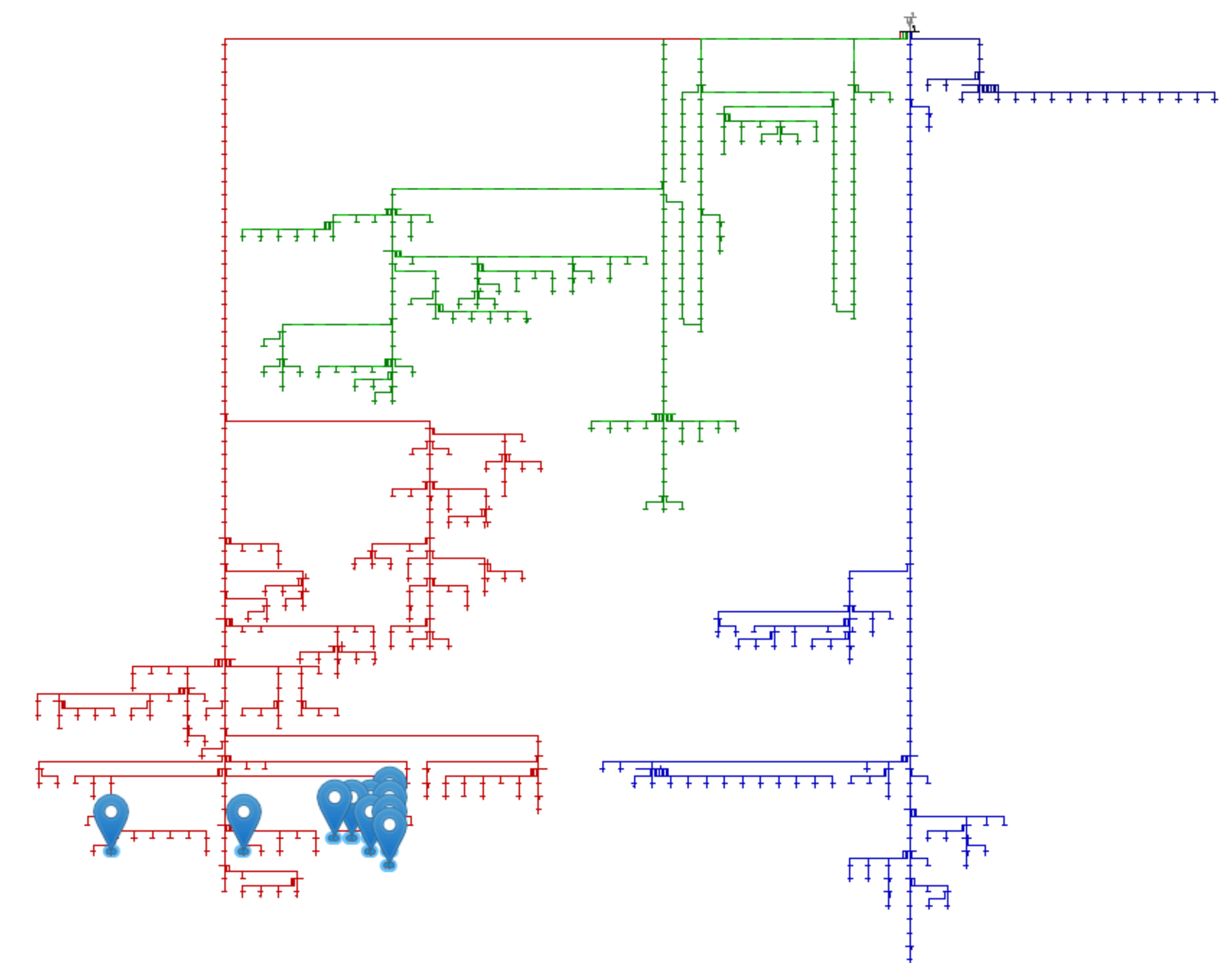
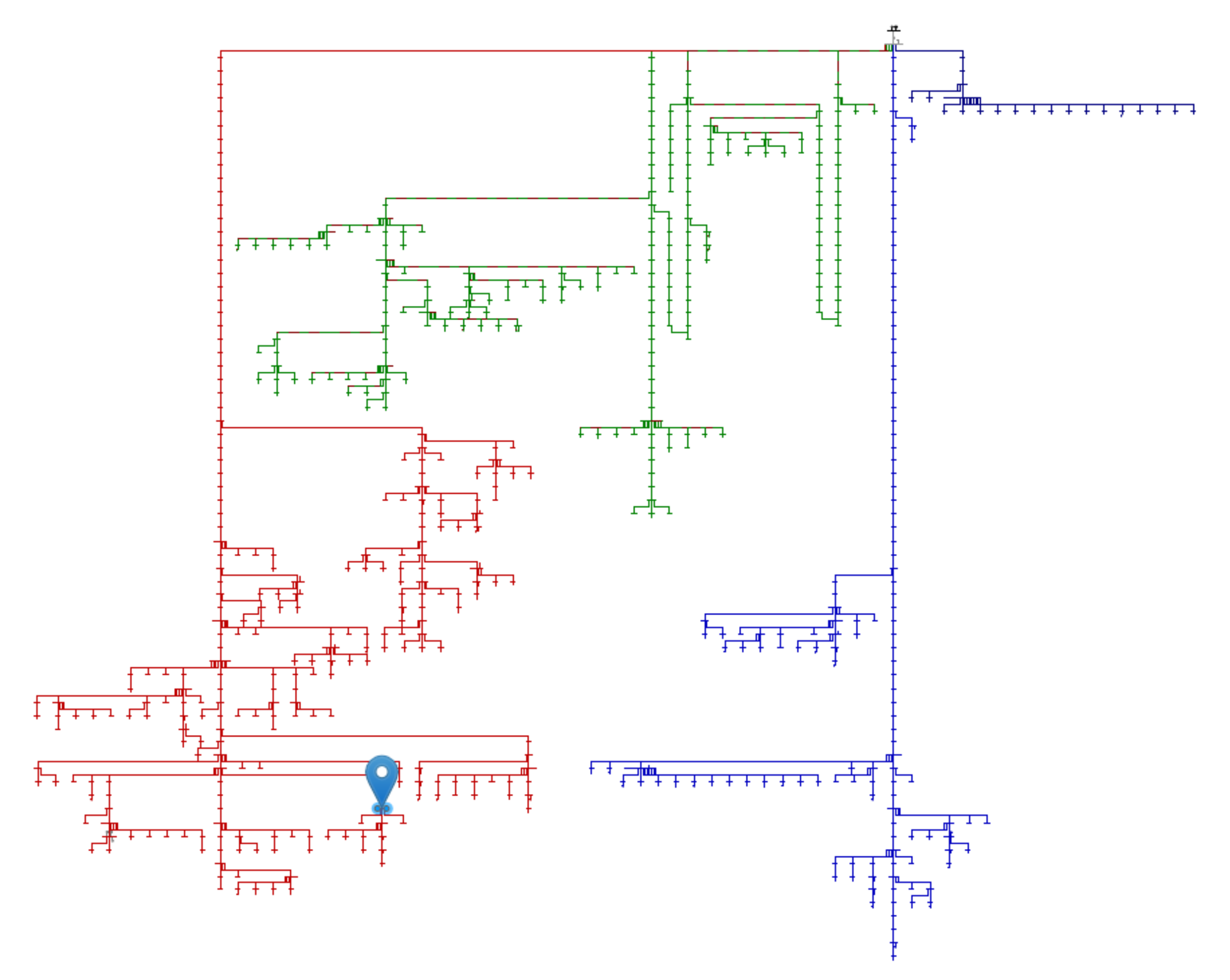
  • Southern Europe rural grid. The methodology was initially developed, tested, and validated in this grid due to the availability of a large amount of quality data.
  • Northern Europe urban-residential grid. The methodology was applied to this network.
  • Central Europe rural-residential grid. The methodology was applied to this network.
  • Southern Europe urban grid. The methodology has been applied to this network.
The proposed methodology, although developed with the Southern Europe rural grid, is flexible to be used in other grids independent of its size, consumer type, or other characteristics. The next subsections show the results of applying the D-STATCOM optimal placement methodology to the distribution grids above-mentioned. The results are also analyzed in these subsections and in Section 4.
The D-STATCOM emulated and optimally placed in this document is being developed by the CIRCE Foundation in the PARITY Project (https://parity-h2020.eu/, accessed on 20 April 2021). This equipment consists of a 4-leg AC/DC converter that allows single-phase controllability, basically for the voltage unbalance compensation. More information about the device is provided in Appendix B.

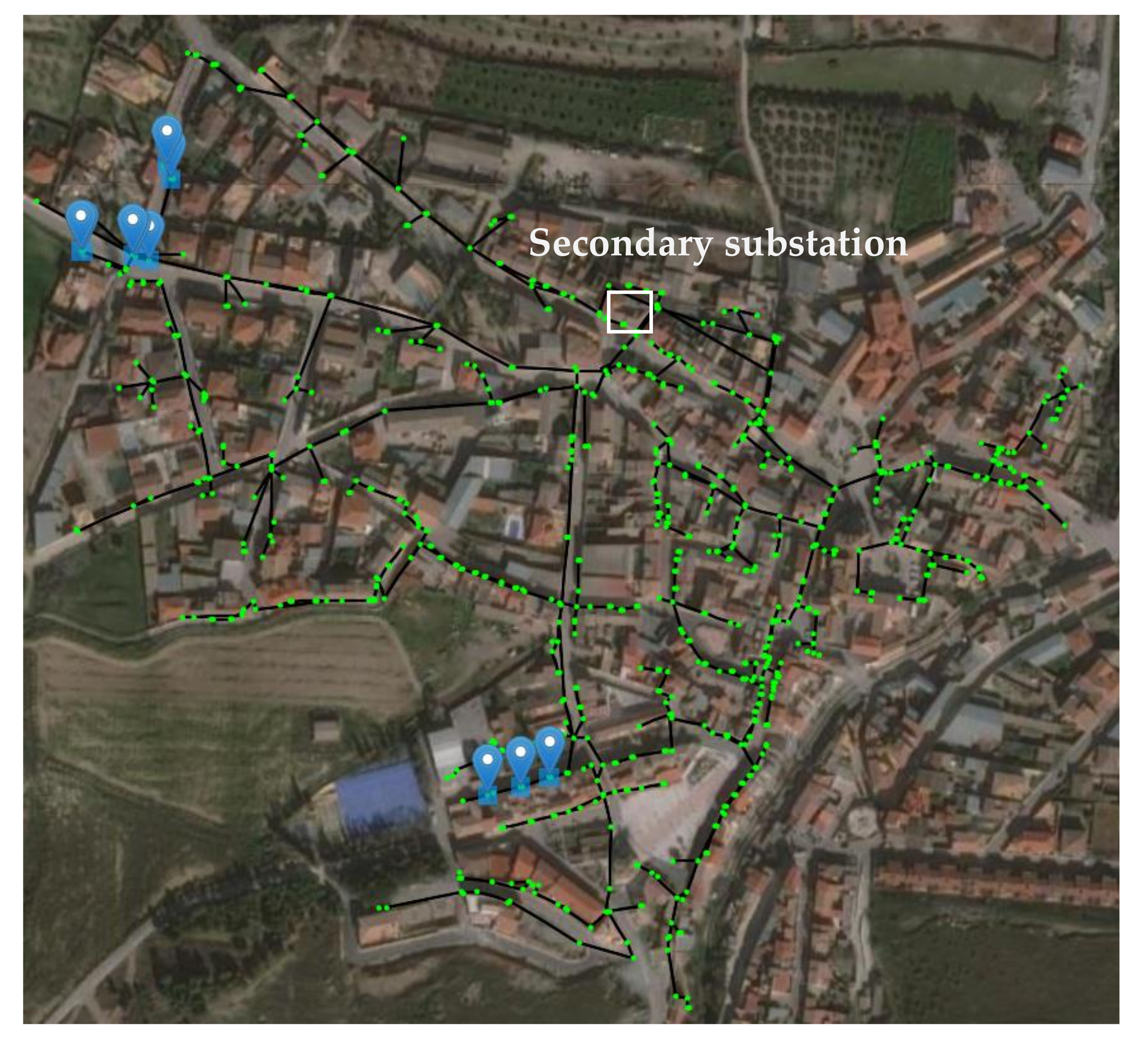
3.1. Southern Europe Rural Grid

This network has 259 supply points including four prosumers (domestic consumers that have solar PV generation devices on their buildings). Besides the generation facilities of the prosumers, there is a 120 kWp photovoltaic plant connected to the distribution network (three-phase, built up from three 40 kWp facilities). Real customer data, obtained from smart meters for one year were used for network analysis and tool development and testing.
As explained in Section 2, the first step of the methodology, the “Unbalance detection stage” generates a database with all the points of the grid presenting unbalances higher than the established limit. This database is sorted according to the values of average and maximum unbalances as well as the number of unbalance events existing during the studied time. Table 1 and Figure 6 identify, characterize, and locate the 10 most unbalanced points of the grid.
In the second step of the methodology, the “D-STATCOM location stage” calculates the grid energy losses reduction, emulating the placement of the D-STATCOM in different points and comparing it with the initial energy losses, when no D-STATCOM is used. Starting from the 10 most unbalanced nodes, a neighborhood search is carried out to find the location in which the loss reductions is the highest (i.e., the optimal D-STATCOM location). Table 2 shows the results of the application of this second stage to the initial 10 nodes, and Table 3 and Table 4 show the results of the neighborhood search application until the optimal node is found. Finally, Figure 7 shows the optimal placement of the D-STATCOM in the Southern Europe rural grid. These tables show the grid energy losses with and without the use of the D-STATCOM and the energy losses reductions, in kWh and in percentage.
As can be seen, the optimal location of the D-STATCOM was not in the initial list of the 10 most suitable points, but was found using the proposed neighborhood search method. This can be because the initially analyzed points had higher average unbalance values, but these unbalances were not continuous and saturated the D-STATCOM, so it could not fully compensate for these high unbalances and the rest of the time, it was not working. On the other hand, the optimal point, although having lower average unbalances, could be more continuous in time and the D-STATCOM was used more efficiently for a longer period of time.
The effect of the D-STATCOM on the network studied was verified and it was observed that the voltage unbalances in the feeder where the equipment had been installed had been reduced, both in terms of value and number of occurrences. The initial three most unbalanced points with the effect of D-STATCOM fell to 19th, 22nd and 23rd ranks of unbalance, as shown in Table 5.
As shown in Table 6 and in Figure 8, the new 10 most unbalanced nodes were located in a different feeder to which the D-STATCOM was located. In fact, these nodes maintained the initial unbalance values, highlighting the local characteristics of voltage unbalances originated by unbalanced demands and the local effect of the D-STATCOM.
Ultimately, in this first grid, the correct behavior of the methodology was verified by applying it to 33 additional nodes and their neighborhood. In total, from the 869 nodes of the grid, the methodology was applied to 33 points and their neighborhoods, 70 nodes in total within the entire grid. Table 7 shows that no nodes with extra energy loss reductions were found, therefore, the proposed method can be considered correct and able to find the optimal location in the analyzed network. This last point, coupled with the characteristics in voltage unbalances (local and at the end of radial feeders suppling energy to single phase consumers), suggests that the proposed process can optimally locate a D-STATCOM in LV distribution grids.

3.2. Northern Europe Urban-Residential Grid

This network has 85 connection points (for consumers, prosumers, and generators). There are five prosumers with generation facilities of 5 or 6 kWp, all of which are three-phase. Among these supply points, there are three photovoltaic generation plants (three-phase and 31 kWp each). Figure 9 shows the location of the 10 most unbalanced nodes and Table 8 shows the energy loss reduction obtained by the D-STATCOM for each of them.
The application of the methodology and the neighborhood search showed no improvements in the energy losses reduction, so the initial best location was the definitive best location for the D-STATCOM in the Northern Europe urban-residential grid, as shown in Figure 10.

3.3. Central Europe Rural-Residential Grid

This network has 25 supply points. Five of these points are prosumers. The photovoltaic generators of the prosumers are three-phase and their power is between 4 and 27 kWp. Figure 11 shows the location of the 10 most unbalanced nodes and Table 9 shows the energy losses reduction achieved by the D-STATCOM in these nodes.
The application of the methodology and the neighborhood search showed no improvements in the energy loss reduction. The initial best location was the definitive one for the D-STATCOM in this grid, as shown in Figure 12.

3.4. Southern Europe Urban Grid

This network has 193 supply points, two of them are prosumers. The photovoltaic generators are three-phase with 14.3375 kWp each. Figure 13 shows the location of the 10 most unbalanced nodes and Table 10 shows the energy loss reduction obtained by the D-STATCOM.
Figure 14 shows the optimal placement of the D-STATCOM in the Southern Europe urban grid. As can be seen, the optimal location of the D-STATCOM was not in the initial list of the 10 most suitable points, but was found using the proposed neighborhood search method. The most suitable point was “Terminal 23” in the neighborhood of “Terminal 27” (see Table 11).

4. Discussion

The proposed method, unlike others mentioned in the literature review in the initial sections of this document, focused on the location of a single D-STATCOM in the low voltage network, while other studies have dealt with the location and sizing of this type of element. In contrast to other works, the present paper focused on the use of the D-STATCOM to avoid voltage unbalance between phases and reduce the associated energy losses. These two points allow for the development of a simple, as opposed to complex, genetic algorithm or PSO and other variants, and an accurate method for the optimal placement of a D-STATCOM of a fixed power to reduce unbalances or voltage and reactive compensation.
The results showed that the algorithm presented allows, in the first stage, for the identification of the network nodes with the highest voltage unbalances (caused by unbalanced consumption) and then to choose among them (and those geographically and electrically close) the one where the effect of the D-STATCOM is most efficient.
The major limitation of the presented method is that it requires a large amount of data: (i) an accurate modeling of the target distribution network is necessary, and (ii) it needs sufficiently long- and representative-time measurements of consumption and generation.
One of the main implications of the developed method, which is both simple and effective, is that the use of D-STATCOM devices in real distribution networks could become more common, given their great potential to avoid or at least reduce the problems that exist or may exist in the low voltage networks of the future.
Table 12 shows the summary of the results of applying a D-STATCOM in the four example grids in their optimal locations, highlighting energy loss reductions and economic savings in each of the grids. As can be seen, the main advantages of the use of this equipment in networks are not directly economic, but technical by improving the balance of the network, the durability of the equipment by working with balanced consumption and voltages, and efficiency by reducing technical losses in the distribution network, which indirectly translates into better remuneration for the DSO, in Spain, for example.
Further developments of the proposed method for the optimal placement of D-STATCOM devices in the short-term can consider:
  • Modeling in more depth the economic aspects of D-STATCOM deployment such as lifetime O&M costs, installation costs, and reactive compensation effect and economic evaluation.
  • Modeling the reactive power compensation and other D-STATCOM functionalities.
In the medium-term, it is proposed to extend the tool to determine not only the optimal location, but also the optimal number of D-STATCOM devices.

5. Conclusions

A high rate of single-phase consumers in low-voltage distribution networks can lead to demand unbalances between phases, resulting in voltage unbalances and increased losses, among other problems. These problems could increase in the near future, as distributed generation technologies are expected to become more widespread. Several techniques have been proposed to avoid, or at least reduce, these problems: demand management, use of electrical energy storage to adapt consumption to hypothetical energy generation, etc. This article proposes the use of D-STATCOM devices to reduce voltage unbalances and take advantage of their characteristics to compensate reactive power in times of balanced voltages.
In order to take advantage of the potential of these D-STATCOM devices, a methodology was developed, applied, and tested for the optimal location of a single D-STATCOM of a predefined power in a low voltage network. The developed method was based on an in-depth analysis of a distribution network to identify the points with the highest unbalances, in average value, throughout the year, and then search in these points and in their neighborhood for the point where the positive effect of the D-STATCOM was greatest. This simple approach is sufficient to solve these voltage unbalance problems, which were concentrated at the ends of long and radial distribution networks in most of the cases. This methodology has been proven to work in four real networks of different characteristics and different locations in Europe.

Author Contributions

Conceptualization, G.F., A.M., and N.G.; Methodology, G.F., A.M., and N.G.; Software, G.F., A.M., and N.G.; Validation, G.F., A.M., and N.G.; Formal analysis, G.F., A.M., and N.G.; Investigation, G.F., A.M., N.G., J.B.-F., and J.M.-C.-A.; Resources, P.L., S.S., E.D., and A.R.; Writing—original draft preparation, G.F., A.M., and N.G.; Writing—review and editing, G.F., A.M., N.G., J.B.-F., J.M.-C.-A., P.L., S.S., E.D., A.R., and D.I.; Visualization, G.F., A.M., N.G., J.B.-F., J.M.-C.-A., P.L., S.S., E.D., A.R., and D.I. All authors have read and agreed to the published version of the manuscript.

Funding

This research has received funding from the European Union’s Horizon 2020 Framework Program for Research and Innovation under grant agreement no. 864319.

Institutional Review Board Statement

Not applicable.

Informed Consent Statement

Not applicable.

Acknowledgments

We thank MONTAJES ELECTRICOS CUERVA-CUERVA Group. E.ON Energilösningar AB & E.ON Energidistribution AB. AZIENDA ELETTRICA DI MASSAGNO (AEM) SA, and DIACHEIRISTIS ELLINIKOU DIKTYOU DIANOMIS ELEKTRIKIS ENERGEIAS AE (HEDNO) for supporting the research carried out and providing information on their distribution grids. We would also like to thank all the project partners for their support and expertise. which was essential for the development of this research.

Conflicts of Interest

The authors declare no conflict of interest.

Nomenclature

PVPhotovoltaic
TSOTransmission System Operator
DSODistribution System Operator
DERDistributed Energy Resource
LVLow Voltage
IREAInternational Renewable Energy Agency
THDTotal Harmonic Distortion
TDDTotal Demand Distortion
PLCPower Line Communication
APLCActive Power Line Conditioner
APFActive Power Filter
SVCStatic VAR Compensator
SVRSet Voltage Regulator
FACTSFlexible AC Transmission Systems
D-STATCOMDistribution Static Synchronous Compensator
VSIVoltage Sensitivity Index
PLIPower Loss Index
PSOParticle Swarm Optimization
GAGenetic Algorithm
HSMHarmony Search Method
ACOAnt Colony Optimization
GWOGrey Wolf Optimizer
LSALightning Search Algorithm
O&MOperations & Maintenance
EVElectric Vehicle

Appendix A

In this annex, a description of the low voltage grids used to develop and test the tool is shown: Southern Europe rural grid, Northern Europe urban-residential grid, Central Europe rural-residential grid, and Southern Europe urban grid. This description is high-level, providing general data, but not personal information or sensitive network or DSO data: main characteristics of transformers and wires, general demand curves of connected users, power of DERs, etc.

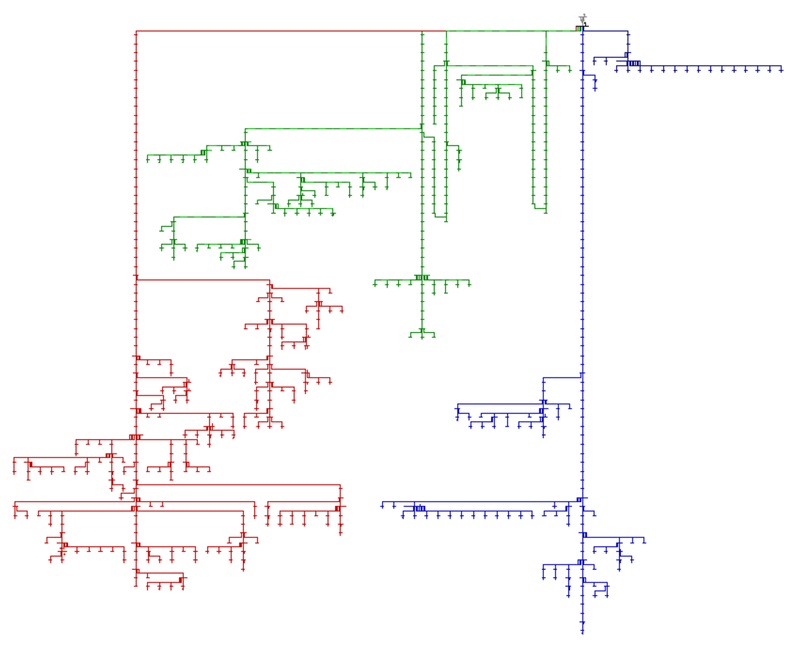
Appendix A.1. Southern Europe Rural Grid

This network has single and three-phase consumers, prosumers, and photovoltaic generators, which makes it representative of future electric grids and makes it a good framework for algorithm development and testing.
Figure A1 shows the one-line diagram of the Southern Europe rural grid network in which each of the branches can be seen in different colors.
Figure A1. Southern Europe rural network topology.
Energies 14 04212 g0a1
Table A1 and Figure A2 show the main characteristics of the transformer and the voltage profile in the low voltage side of the secondary substation in a representative day.
Table A1. Characteristics of the Southern Europe rural grid’s secondary substation.
NameHigh Voltage (kV)Low Voltage (kV)Rated Power (MVA)
Secondary substation200.40.4
Figure A2. Voltage profile in the secondary substation of the Southern Europe rural grid, low voltage side.
Energies 14 04212 g0a2
All the lines of the network have been modeled according to the values in Table A2. This table shows the characteristics of the cables used: conductor voltage, maximum allowed current, cable type, resistance, reactance, and inductance.
Table A2. Southern Europe rural grid conductor types.
Conductor TypeVoltage (kV)Current (kA)3-Phase or 1-PhaseR (Ohm/km)X (Ohm/km)L (mH/km)
RV 2 × 25 AL0.40.0741-Phase1.440.0780.2482817
RV 2 × 50 AL0.40.1051-Phase0.770.07770.2473268
RV 3 × 150 AL0.40.23-Phase0.2490.0720.2291831
RV 3 × 25 AL0.40.0743-Phase1.440.0780.2482817
RV 3 × 50 AL0.40.1053-Phase0.770.07770.2473268
RV 4 × 50 AL0.40.1053-Phase0.770.07770.2473268
RV 4 × 95 AL0.40.1553-Phase0.390.07330.2333211
RZ 3 × 16 CU0.40.0751-Phase1.450.08130.2587859
RZ 3 × 6 CU0.40.0533-Phase3.950.09010.2867972
RZ 4 × 10AL0.40.0543-Phase3.610.0860.2737465
RZ 4 × 16 AL0.40.0583-Phase2.270.08130.2587859
RZ 4 × 25 AL0.40.0743-Phase1.440.0780.2482817
The distribution network has 259 supply points. Four of them are prosumers (PV generation in domestic buildings). These loads are organized into six different power branches connected to the secondary substation.
Real customer measurements were used for network analysis and tool development and testing. These measurements were obtained from smart meters for one year. As an example, Figure A3 shows a single-phase consumption profile example of two customers:
Figure A3. Active power profiles of different consumers.
Energies 14 04212 g0a3
In addition to the prosumers’ generation facilities, there is a 120 kWp photovoltaic plant (three-phase, built up from three 40 kWp facilities) connected to the distribution network, connected through three inverters (PV1, PV2, and PV3 in Table A3).
Table A3. PV generators in Southern Europe rural grid.
Generator3-Phase or 1-PhaseRated Power (kWp)
PV_gen_13-Phase40
PV_gen_23-Phase40
PV_gen_33-Phase40
PV_pros_11-Phase3.3
PV_pros_21-Phase3.3
PV_pros_31-Phase3.3
PV_pros_41-Phase3.3

Appendix A.2. Northern Europe Urban-Residential Grid

This network has different type of consumers: family houses, distributed solar PV prosumers, and different types of consumption points as outdoor swimming pools and EVs. This combination of consumers, generators, and consumption technologies makes this grid representative to be used as a test bed for the D-STATCOM optimal placement tool. Figure A4 shows the one-line diagram of the Northern Europe urban-residential network.
Figure A4. Northern Europe urban-residential network topology.
Energies 14 04212 g0a4
Table A4 summarizes the characteristics of the secondary substation transformer.
Table A4. Characteristics of the Northern Europe urban-residential grid’s secondary substation.
NameHigh Voltage (kV)Low Voltage (kV)Rated Power (MVA)
MV/LV Transformer100.40.8
Table A5 shows the characteristics of the cables used: conductor voltage, maximum allowed current, cable type, resistance, reactance, and inductance.
Table A5. Northern Europe urban-residential grid conductor types.
Conductor TypeVoltage (kV)Current (kA)3-Phase or 1-PhaseR (Ohm/km)X (Ohm/km)L (mH/km)
AXQJ 4 × 240/1460.60.73-Phase0.1250.010.0318
N1XV 4 × 950.60.3083-Phase0.1930.010.0318
N1XV 5 × 160.60.0983-Phase1.150.010.0318
N1XV 5 × 100.60.063-Phase1.830.010.0318
In this network, as not all the consumption profiles were available, different common profiles for consumers, electric vehicles, and outdoor swimming pools have been developed and considered:
  • Figure A5 shows an example profile of a consumer of 5 MWh per year. To see consumption in more detail, the 24-h profile is shown in Figure A6.
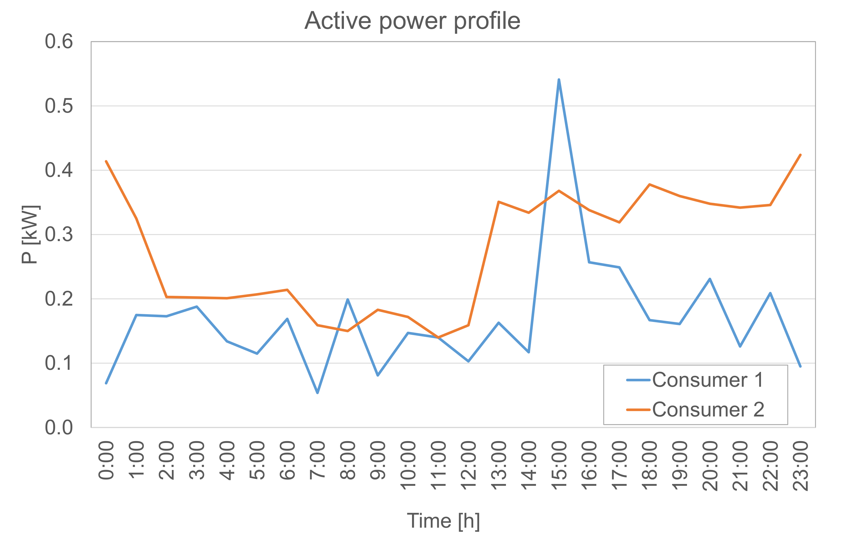
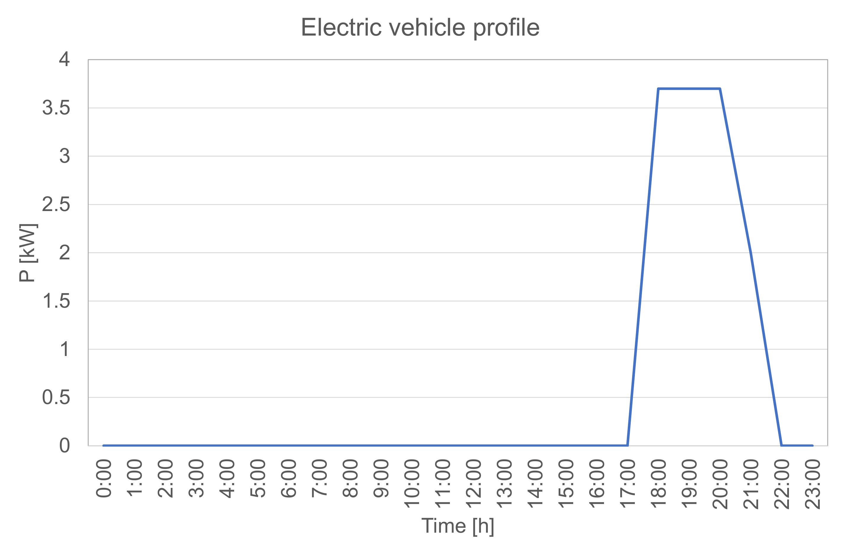
  • Figure A7 shows the proposed consumption of an EV in one day. As a simplification, it has been supposed that the same charging profile for the entire year of study and for all users.
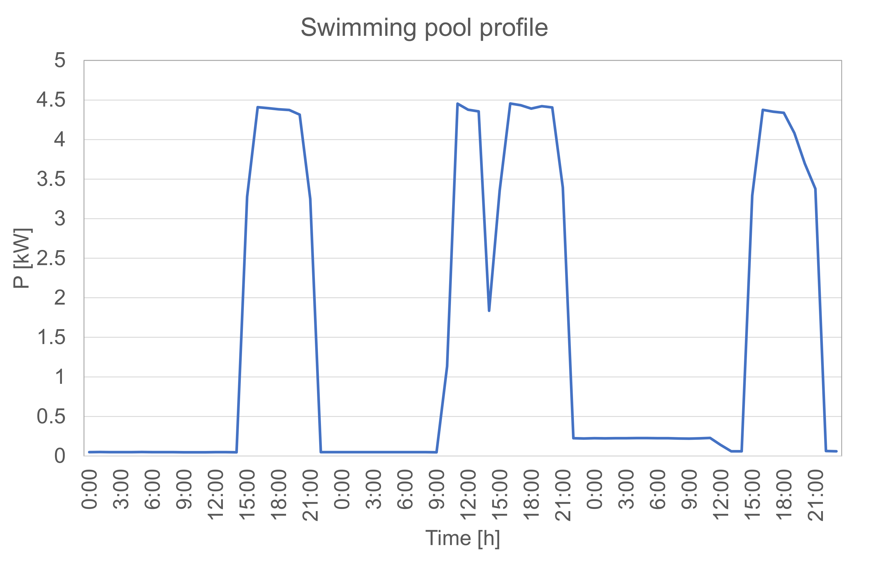
  • In Figure A8, the consumption of an outdoor swimming pool is shown. The operation of this demand point is supposed to cover seven months, from April to September.
Figure A5. Northern Europe urban-residential grid for the 5 MWh/year consumer profile for a full year.
Energies 14 04212 g0a5
Figure A6. Northern Europe urban-residential grid for the 5 MWh/year consumer profile for a day.
Energies 14 04212 g0a6
Figure A7. Northern Europe urban-residential grid EV profile for a day.
Energies 14 04212 g0a7
Figure A8. Northern Europe urban-residential grid outdoor swimming pool profile for three days.
Energies 14 04212 g0a8
The Northern Europe urban-residential network has 85 supply points (consumption and generation). Among them, there are three photovoltaic generation plants whose main characteristics are shown in Table A6. On the other hand, there are customers who generate for their self-consumption (prosumers). In this network, there are five prosumers, who have a single smart meter so their profile is the sum of the profile consumed + generating profile by the photovoltaic. The summary of photovoltaic generation can be seen in Table A7.
Table A6. PV generators in the Northern Europe urban-residential grid.
Generator3-Phase or 1-PhaseRated Power (kWp)
PV_ SR13-Phase31
PV_ SR23-Phase31
PV_SR33-Phase31
Table A7. Prosumers PV generation in the Northern Europe urban-residential grid.
Prosumer3-Phase or 1-PhaseRated Power (kWp)
13-Phase5
23-Phase6
33-Phase6
43-Phase6
53-Phase6

Appendix A.3. Central Europe Rural-Residential Grid

This network has consumers, prosumers, and distributed generation. Figure A9 shows the one-line diagram of the Central Europe rural-residential network.
Figure A9. Central Europe rural-residential network topology.
Energies 14 04212 g0a9
Table A8 summarizes the characteristics of the secondary substation transformer.
Table A8. Characteristics of the Central Europe rural-residential grid’s secondary substation.
NameHigh Voltage (kV)Low Voltage (kV)Rated Power (MVA)
Secondary substation16.80.60.63
Table A9 shows the characteristics of the types of cables used: conductor voltage, maximum allowed current, cable type, resistance, reactance, and capacitance.
Table A9. Central Europe rural-residential grid conductor types.
Conductor TypeVoltage (kV)Current (kA)3-Phase or 1-PhaseR (Ohm/km)X (Ohm/km)C (µF/km)
AXQJ 4 × 40/1460.60.73-Phase0.1250.010.0318
GKN 3 × 95/95 CU0.60.3163-Phase0.2250.070.338
GKN 3 × 25/25 CU0.60.1513-Phase0.8420.080.272
GKN 3 × 50/50 CU0.60.2153-Phase0.4490.070.298
GKN 3 × 150/150 CU0.60.43-Phase0.1460.070.349
The distribution network has 25 supply points. Five of them are prosumers (PV generation in domestic buildings). The photovoltaic generators’ main characteristics are shown in Table A10.
Table A10. PV generators in Central Europe rural-residential grid.
Generator3-Phase or 1-PhaseRated Power (kWp)
PV_13-Phase4
PV_23-Phase27
PV_33-Phase9
PV_43-Phase14
PV_53-Phase10

Appendix A.4. Southern Europe Urban Grid

Figure A10 shows the one-line diagram of the Southern Europe urban grid.
Figure A10. Southern Europe urban grid topology.
Energies 14 04212 g0a10
Table A11 summarizes the characteristics of the secondary substation transformer.
Table A11. Characteristics of the Southern Europe urban grid’s secondary substation.
NameHigh Voltage (kV)Low Voltage (kV)Rated Power (MVA)
Secondary substation200.40.63
Table A12 shows the characteristics of the types of cables used: conductor voltage, maximum allowed current, cable type, resistance, reactance, and inductance.
Table A12. Southern Europe urban grid conductor types.
Conductor TypeVoltage (kV)Current (kA)3-phase or 1-phaseR (Ohm/km)X (Ohm/km)L (mH/km)
3 × 150 AL + 50 CU XLPE0.60.2930.2060.120.3819
4 × 120 AL + 25 AL0.60.2230.2530.10.3183
4 × 35 + 16 AL0.60.05830.08130.08130.2587
The distribution network has 193 supply points. Two of them are prosumers (PV generation in domestic buildings). The photovoltaic generators’ main characteristics are shown in Table A13.
Table A13. PV generators in Southern Europe urban grid network.
GeneratorPhaseRated Power (kWp)
PV_3191000153-phase14.3375
PV_3191000163-phase14.3375

Appendix B

The D-STATCOM emulated and optimally placed in this document is being developed by CIRCE Foundation in the PARITY Project. This equipment consists of a 4-leg AC/DC converter, similar to the one shown in Figure A11. This 4-leg D-STATCOM works as three single-phase converters (ia, ib, ic show current phases in the figure) connected through their DC-link [58]. In a single-phase converter, the current path is closed through the neutral wire. Unlike three single-phase converters, in a 4-leg converter, the three neutral wires merge into one (ia + ib + ic are the current in the neutral), through which the currents of the three phases will return. Thus, unlike common 3-wire converters, a 4-wire D-STATCOM allows single-phase controllability, extending the operating points to unbalanced loads and allowing independent active and reactive power setpoints in each phase.
Figure A11. The 4-leg bi-level AC/DC topology. The D-STATCOM developed has a three-level topology, which achieves a lower harmonic content and a passive component size reduction compared to bi-level converters.
Energies 14 04212 g0a11
The 30 kVA D-STATCOM under development does not have energy storage, load or power source and, consequently, the energy entering one or two phases must be returned to the grid through the others [59]. This operation and the constructive characteristics makes D-STATCOM of a great potential as DER to fulfil the next functions:
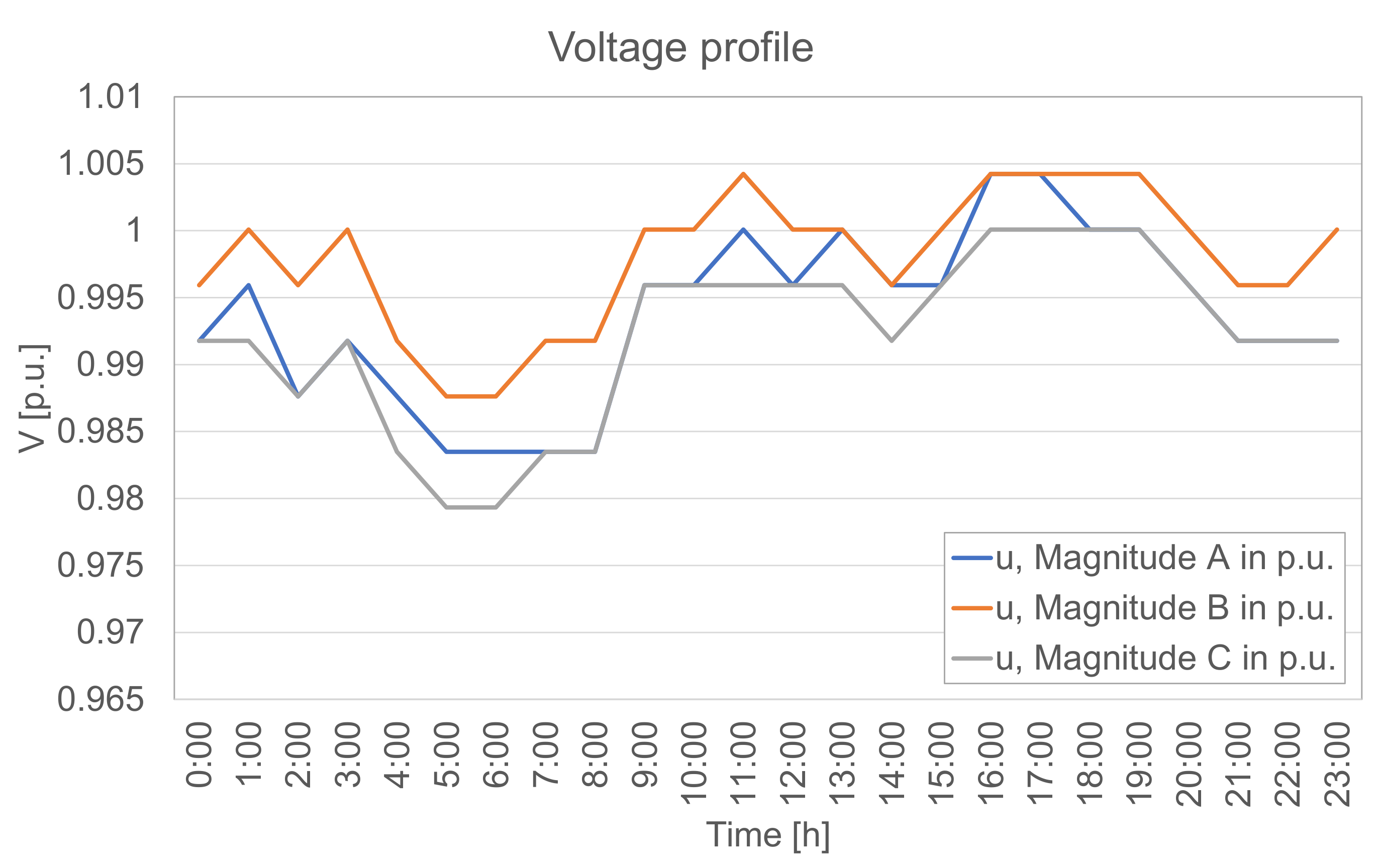
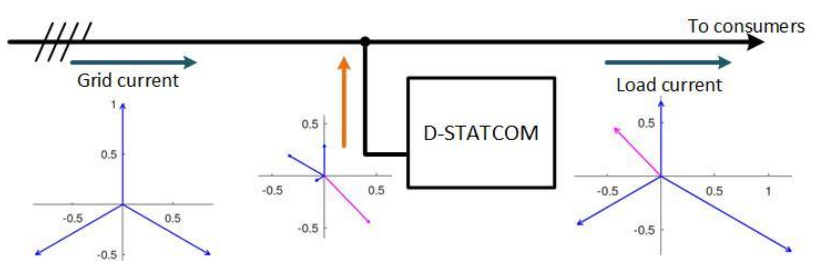
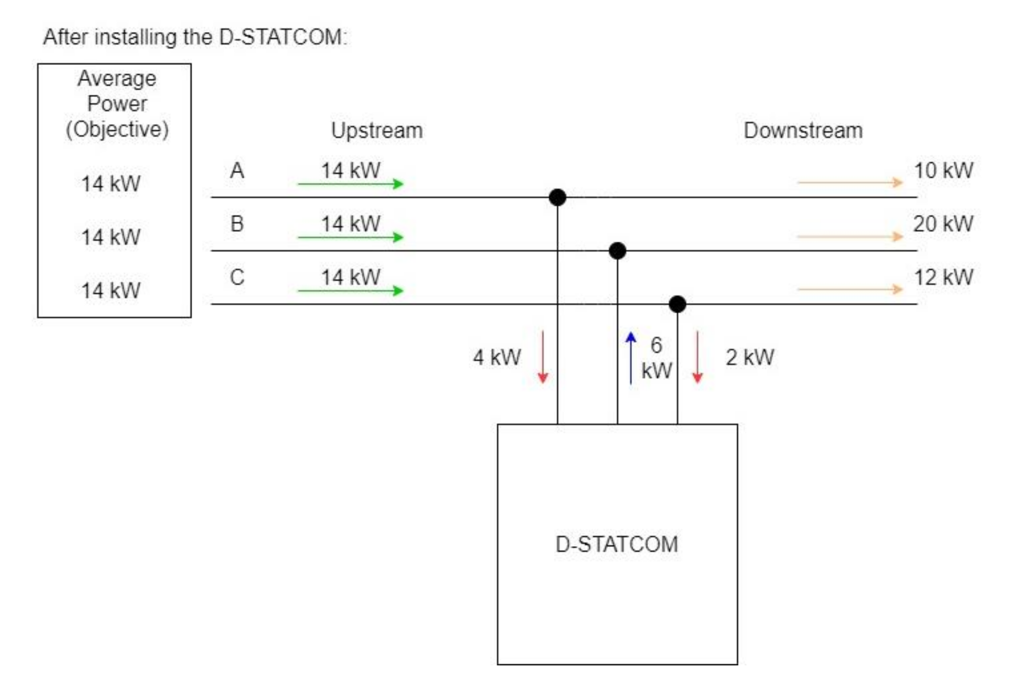
  • Line current balancing. As above-mentioned, single phase loads produce different current flows in each phase of the network and also different voltage drops in each phase, affecting the power supply quality. This unbalance also increases the neutral current, requiring an oversizing of neutral cables and reducing energy efficiency and making failures more frequent. Figure A12 shows that the current injected by the D-STATCOM compensates for the unbalanced current demanded by consumers, so that current upstream is balanced and neutral current has been removed.
  • Reactive compensation. Related to the previous point, reactive power compensation reduces power loses and voltage drops, improving the network operation.
  • Voltage regulation. Similar to large STATCOMs used in transport network, a D-STATCOM can take advantage of the Ferranti effect to support voltage regulation in grid lines. In addition, this regulation can be carried out in a single-phase mode, applying an independent volt-var curve in each phase.
Another two benefits of the D-STATCOM to be highlighted are that due to the low harmonic emission, no additional filters are required and its high switching frequency over the audible spectrum makes it completely silent in operation and compatible with inhabited environments. Moreover, as Figure A12 shows, the D-STATCOM is shunt connected to the grid, allowing a safe disconnection when its operation is not required, avoiding power losses.
Figure A12. Line current balancing (phase currents in blue, neutral current in pink). The unbalanced current demanded by consumers is measured by the D-STATCOM, that calculates and injects the current required to balance the line.
Energies 14 04212 g0a12

References

  1. The Intergovernmental Panel on Climate Change (IPCC). In Global Warming of 1.5 °C; IPCC: Geneva, Switzerland, 2018.
  2. Batel, S. Research on the social acceptance of renewable energy technologies: Past, present and future. Energy Res. Social Sci. 2020, 68, 101544. [Google Scholar] [CrossRef]
  3. The European Parliament and the Council of the European Union. Directive 2009/28/EC of 23 April 2009; European Parliament: Brussels, Belgium, 2009. [Google Scholar]
  4. European Commission. Available online: https://ec.europa.eu/energy/topics/energy-strategy/clean-energy-all-europeans_en (accessed on 15 October 2020).
  5. Verzijlbergh, R.; Vries, L.D.; Dijkema, G.; Herder, P. Institutional challenges caused by the integration of renewable energy sources in the European electricity sector. Renew. Sustain. Energy Rev. 2017, 75, 660–667. [Google Scholar] [CrossRef] [Green Version]
  6. Tech, V. Distributed Generation Educational Module. Available online: https://www.dg.history.vt.edu/ch1/introduction.html (accessed on 14 October 2020).
  7. European Commission. Study on the Effective Integration of Distributed; European Commission: Brussels, Belgium, 2015. [Google Scholar]
  8. Kharrazi, A.; Sreeram, V.; Mishra, Y. Assessment techniques of the impact of grid-tied rooftop photovoltaic generation on the power quality of low voltage distribution network—A review. Renew. Sustain. Energy Rev. 2020, 120, 109643. [Google Scholar] [CrossRef]
  9. Gandhi, O.; Zhang, W.; Rodríguez-Gallegos, C.D.; Srinivasan, D.; Reindl, T. Continuous optimization of reactive power from PV and EV in distribution system. In Proceedings of the 2016 IEEE Innovative Smart Grid Technologies—Asia (ISGT-Asia), Melbourne, Australia, 28 November–1 December 2016. [Google Scholar]
  10. Aziz, T.; Ketjoy, N. PV Penetration Limits in Low Voltage Networks and Voltage Variations. IEEE Access 2017, 5, 16784–16792. [Google Scholar] [CrossRef]
  11. International Energy Agency (IEA). Impacts of Power Penetration from Photovoltaic Power Systems in Distribution Networks; IEA: Paris, France, 2002. [Google Scholar]
  12. Masoum, A.S.; Moses, P.S.; Masoum, M.A.; Abu-Siada, A. Impact of rooftop PV generation on distribution transformer and voltage profile of residential and commercial networks. In Proceedings of the 2012 IEEE PES Innovative Smart Grid Technologies (ISGT), Washington, DC, USA, 16–20 January 2012; pp. 1–7. [Google Scholar]
  13. Zhang, C.; Ding, Y.; Nordentoft, N.C.; Pinson, P.; Østergaard, J. FLECH: A Danish market solution for DSO congestion. J. Mod. Power Syst. Clean Energy 2014, 2, 126–133. [Google Scholar] [CrossRef] [Green Version]
  14. Haque, A.N.M.M.; Nguyen, P.H.; Kling, W.L.; Bliek, F.W. Congestion management in smart distribution network. In Proceedings of the 2014 49th International Universities Power Engineering Conference (UPEC), Cluj-Napoca, Romania, 2–5 September 2014. [Google Scholar]
  15. Phuttapatimok, S.; Sangswang, A.; Seapan, M.; Chenvidhya, D.; Kirtikara, K. Evaluation of fault contribution in the presence of PV grid-connected systems. In Proceedings of the 33rd IEEE Photovoltaic Specialists Conference, San Diego, CA, USA, 11–16 May 2008; pp. 1–5. [Google Scholar]
  16. Rafi, F.H.M.; Hossain, M.J.; Rahman, M.S.; Taghizadeh, S. An overview of unbalance compensation techniques using power electronic converters for active distribution systems with renewable generation. Renew. Sustain. Energy Rev. 2020, 125, 109812. [Google Scholar] [CrossRef]
  17. Almeida, D.; Abeysinghe, A.; Ekanayake, J.B. Analysis of rooftop solar impacts on distribution networks. Ceylon J. Sci. 2019, 48, 103–112. [Google Scholar] [CrossRef] [Green Version]
  18. Schwanz, D.; Möller, F.; Rönnberg, S.K.; Meyer, J.; Bollen, M.H.J. Stochastic Assessment of Voltage Unbalance Due to Single-Phase-Connected Solar Power. IEEE Trans. Power Deliv. 2016, 32, 852–861. [Google Scholar] [CrossRef]
  19. Garrett, D.; Jeter, S. A photovoltaic voltage regulation impact investigation technique. I. Model development. IEEE Trans. Energy Convers. 1989, 4, 47–53. [Google Scholar] [CrossRef]
  20. Wang, L.; Yan, R.; Saha, T.K. Voltage regulation challenges with unbalanced PV integration in low voltage distribution systems and the corresponding solution. Appl. Energy 2019, 256, 113927. [Google Scholar] [CrossRef]
  21. Mateo, C.; Cossenta, R.; Gómez, T.; Prettico, G.; Frías, P.; Fulli, G.; Meletiou, A.; Postigo, F. Impact of solar PV self-consumption policies on distribution networks and regulatory implications. Sol. Energy 2018, 176, 62–72. [Google Scholar] [CrossRef]
  22. Sauhats, A.; Zemite, L.; Petrichenko, L.; Moshkin, I.; Jasevics, A. Estimating the Economic Impacts of Net Metering Schemes for Residential PV Systems with Profiling of Power Demand, Generation, and Market Prices. Energies 2018, 11, 3222. [Google Scholar] [CrossRef] [Green Version]
  23. Huang, S.; Wu, Q.; Liu, Z.; Nielsen, A.H. Review of congestion management methods for distribution networks with high penetration of distributed energy resources. In Proceedings of the IEEE PES Innovative Smart Grid Technologies, Europe, Istanbul, Turkey, 12–15 October 2014; pp. 1–6. [Google Scholar]
  24. Marini, A.; Ghazizadeh, M.S.; Mortazavi, S.S.; Piegari, L. A harmonic power market framework for compensation management of DER based active power filters in microgrids. Electr. Power Energy Syst. 2019, 113, 916–931. [Google Scholar] [CrossRef]
  25. Torres, I.C.; Negreiros, G.F.; Tiba, C. Theoretical and Experimental Study to Determine Voltage Violation, Reverse Electric Current and Losses in Prosumers Connected to Low-Voltage Power Grid. Energies 2019, 12, 4568. [Google Scholar] [CrossRef] [Green Version]
  26. Hong, B.; Li, Q.; Miao, W.; Yan, H.; Liu, J. Energy Storage Application in Improving Distribution Network’s Solar Photovoltaic (PV) Adoption Capability. Energy Procedia 2018, 145, 472–477. [Google Scholar] [CrossRef]
  27. Bremdal, B.A.; Sæle, H.; Mathisen, G.; Degefa, M.Z. Flexibility offered to the distribution grid from households with a photovoltaic panel on their roof: Results and experiences from several pilots in a Norwegian research project. In Proceedings of the 2018 IEEE International Energy Conference (ENERGYCON), Limassol, Cyprus, 3–7 June 2018; pp. 1–6. [Google Scholar]
  28. Wind EUROPE. Repowering and Lifetime Extension: Making the Most of Europe’s Wind Energy Resource; Wind EUROPE: Brussels, Belgium, 2017. [Google Scholar]
  29. Ren, B.; Zhang, M.; An, S.; Sun, X. Local Control Strategy of PV Inverters for Overvoltage Prevention in Low Voltage Feeder. In Proceedings of the 2016 IEEE 11th Conference on Industrial Electronics and Applications, Hefei, China, 5–7 June 2016; pp. 2071–2075. [Google Scholar]
  30. Fernández, G.; Galan, N.; Marquina, D.; Martínez, D.; Sanchez, A.; López, P.; Bludszuweit, H.; Rueda, J. Photovoltaic Generation Impact Analysis in Low Voltage Distribution Grids. Energies 2020, 13, 4347. [Google Scholar] [CrossRef]
  31. Jeong, Y.-C.; Lee, E.-B.; Alleman, D. Reducing Voltage Volatility with Step Voltage Regulators: A Life-Cycle Cost Analysis of Korean Solar Photovoltaic Distributed Generation. Energies 2019, 12, 652. [Google Scholar] [CrossRef] [Green Version]
  32. Kahingala, T.D.; Perera, S.; Agalgaonkar, A.P.; Jayatunga, U. STATCOM Based Network Voltage Unbalance Mitigation for Sub-Transmission Networks. In Proceedings of the IEEE Innovative Smart Grid Technologies—Asia (ISGT Asia), Chengdu, China, 21–24 May 2019; pp. 2624–2628. [Google Scholar]
  33. Kahingala, T.D.; Perera, S.; Jayatunga, U.; Agalgaonkar, A.P. Network-Wide Influence of a STATCOM Configured for Voltage Unbalance Mitigation. IEEE Trans. Power Deliv. 2020, 35, 1602–1605. [Google Scholar] [CrossRef]
  34. Rodríguez, A.; Bueno, E.J.; Mayor, Á.; Rodríguez, F.J.; García-Cerrada, A. Voltage Support Provided by STATCOM in Unbalanced Power Systems. Energies 2014, 7, 1003–1026. [Google Scholar] [CrossRef] [Green Version]
  35. Afzal, M.M.; Khan, M.A.; Hassan, M.A.S.; Wadood, A.; Uddin, W.; Hussain, S.; Rhee, S.B. A Comparative Study of Supercapacitor-Based STATCOM in a Grid-Connected Photovoltaic System for Regulating Power Quality Issues. Sustainability 2020, 12, 6781. [Google Scholar] [CrossRef]
  36. Kotsampopoulos, P.; Georgilakis, P.; Lagos, D.T.; Kleftakis, V.; Hatziargyriou, N. FACTS Providing Grid Services: Applications and Testing. Energies 2019, 12, 2554. [Google Scholar] [CrossRef] [Green Version]
  37. Yuvaraj, T.; Devabalaji, K.R.; Ravi, K. Optimal Placement and Sizing of DSTATCOM Using Harmony Search Algorithm. Energy Procedia 2015, 79, 759–765. [Google Scholar] [CrossRef] [Green Version]
  38. Sirjani, R. Optimal placement and sizing of distribution static compensator (D-STATCOM) in electric distribution networks: A review. Renew. Sustain. Energy Rev. 2017, 77, 688–694. [Google Scholar] [CrossRef]
  39. Hussain, S.M. An analytical approach for optimal location of DSTATCOM in radial distribution system. In Proceedings of the 2013 International Conference on Energy Efficient Technologies for Sustainability, ICEETS 2013, Nagercoil, India, 10–12 April 2013. [Google Scholar]
  40. Tuzikova, V.; Tlusty, J.; Muller, Z. A Novel Power Losses Reduction Method Based on a Particle Swarm Optimization Algorithm Using STATCOM. Energies 2018, 11, 2851. [Google Scholar] [CrossRef] [Green Version]
  41. Sirjani, R. Optimal Placement and Sizing of PV-STATCOM in Power Systems Using Empirical Data and Adaptive Particle Swarm Optimization. Sustainability 2018, 10, 727. [Google Scholar] [CrossRef] [Green Version]
  42. Shirmohammadi, D.; Wollenberg, B.; Vojdani, A.; Sandrin, P.; Pereira, M.; Rahimi, F.; Schneider, T.; Stott, B. Transmission dispatch and congestion management in the emerging energy market structures. IEEE Trans. Power Syst. 1998, 13, 1466–1474. [Google Scholar] [CrossRef]
  43. Oloulade, A.; Imano, A.M.; Viannou, A.; Tamadaho, H. Optimization of the number, size and placement of D-STATCOM in radial distribution network using Ant Colony Algorithm. Am. J. Eng. Res. Rev. 2018, 1, 12. [Google Scholar]
  44. Gupta, A.R.; Kumar, A. Impact of various load models on D-STATCOM allocation in DNO operated distribution network . Procedia Comput. Sci. 2018, 125, 862–870. [Google Scholar]
  45. Gupta, A.R.; Kumar, A. Impact of DG and D-STATCOM Placement on Improving the Reactive Loading Capability of Mesh Distribution System. Procedia Technol. 2016, 25, 676–683. [Google Scholar] [CrossRef] [Green Version]
  46. Gupta, A.R.; Kumar, A. Energy Saving Using D-STATCOM Placement in Radial Distribution System under Reconfigured Network. Energy Procedia 2016, 90, 124–136. [Google Scholar] [CrossRef]
  47. Gupta, A.R.; Kumar, A. Optimal placement of D-STATCOM using sensitivity approaches in mesh distribution system with time variant load models under load growth. Ain Shams Eng. J. 2018, 9, 783–799. [Google Scholar] [CrossRef] [Green Version]
  48. Gupta, A.R.; Kumar, A. Impact of D-STATCOM Placement on Improving the Reactive Loading Capability of Unbalanced Radial Distribution System. Procedia Technol. 2016, 25, 759–766. [Google Scholar] [CrossRef] [Green Version]
  49. Rezaeian-Marjani, S.; Galvani, S.; Talavat, V.; Farhadi-Kangarlu, M. Optimal allocation of D-STATCOM in distribution networks including correlated renewable energy sources. Int. J. Electr. Power Energy Syst. 2020, 122, 106178. [Google Scholar] [CrossRef]
  50. Mohamed, M.A.E.S.; Mohammed, A.A.E.; Abd Elhamed, A.M.; Hessean, M.E. Optimal Allocation of Photovoltaic Based and DSTATCOM in a Distribution Network under Multi Load Levels. Eur. J. Eng. Res. Sci. 2019, 4, 114–119. [Google Scholar] [CrossRef]
  51. Thangaraj, Y.; Kuppan, R. Multi-objective simultaneous placement of DG and DSTATCOM using novel lightning search algorithm. J. Appl. Res. Technol. 2017, 15, 477–491. [Google Scholar] [CrossRef]
  52. Singh, B.; Yadav, M.K. GA for enhancement of system performance by DG incorporated with D-STATCOM in distribution power networks. J. Electr. Syst. Inf. Technol. 2018, 5, 388–426. [Google Scholar] [CrossRef]
  53. Castiblanco-Pérez, C.M.; Toro-Rodríguez, D.E.; Montoya, O.D.; Giral-Ramírez, D.A. Optimal Placement and Sizing of D-STATCOM in Radial and Meshed Distribution Networks Using a Discrete-Continuous Version of the Genetic Algorithm. Electronics 2021, 10, 1452. [Google Scholar] [CrossRef]
  54. Ruiz, J.L. Metaheurísticas para el Análisis de Datos Masivos en el Ámbito del Transporte por Carretera; Universidad Politécnica de Madrid: Madrid, Spain, 2017. [Google Scholar]
  55. DIgSILENT | POWER SYSTEM SOLUTIONS. Available online: https://www.digsilent.de/en/ (accessed on 21 April 2021).
  56. CENELEC. EN 50160—Voltage Characteristics of Electricity Supplied by Public Electricity Networks; CENELEC: Brussels, Belgium, 2011. [Google Scholar]
  57. Block, I. About the Method of Unification of the Program-Algorithmic Model of Multi-Agent Optimization Methods Using the Example of the Particle Swarm Method. Available online: https://www.sciencedirect.com/science/article/abs/pii/S0169743915002117 (accessed on 15 April 2021).
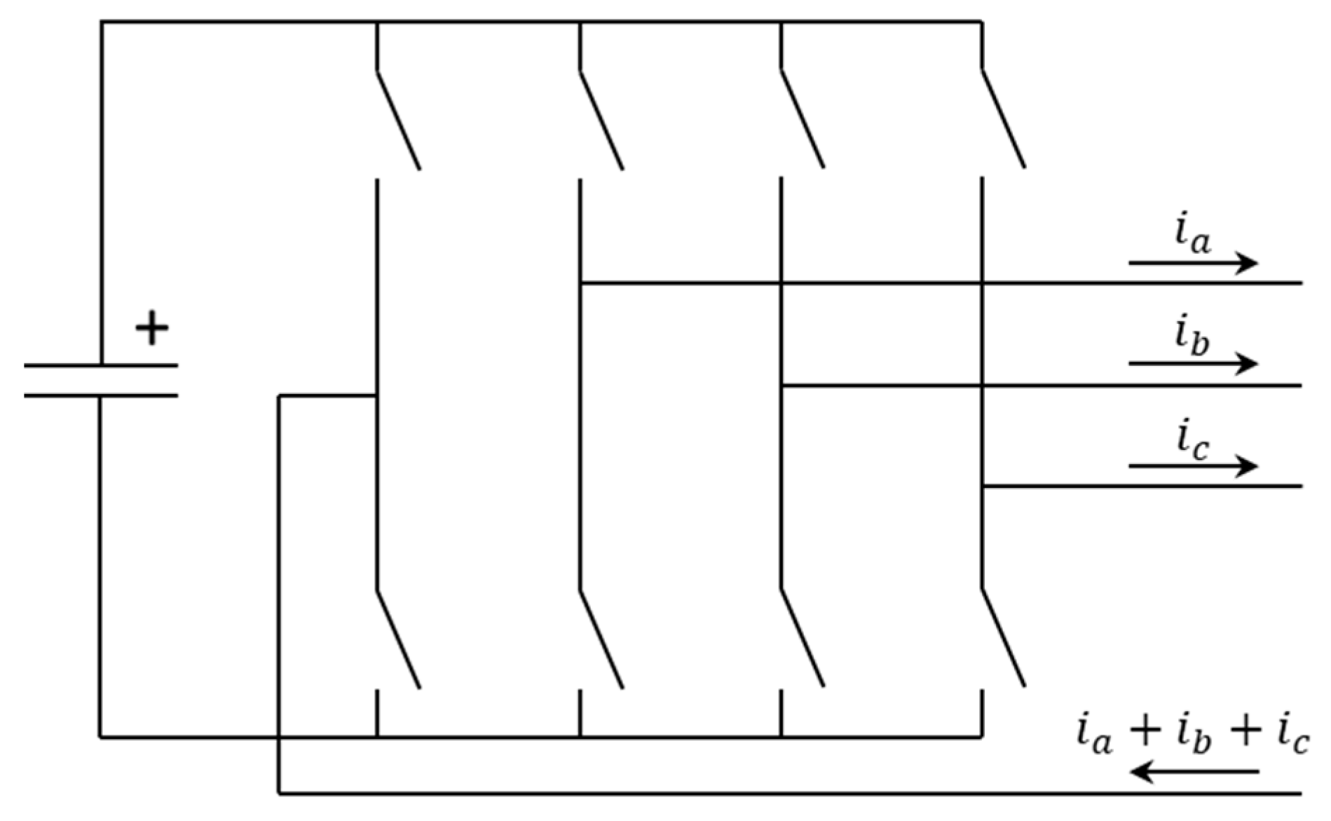
  58. Ryan, M.J.; De Doncker, R.W.; Lorenz, R.D. Decoupled control of a four-leg inverter via a new 4/spl times/4 transformation matrix. IEEE Trans. Power Electron. 2001, 16, 694–701. [Google Scholar] [CrossRef] [Green Version]
  59. Ballestín, J. 4-Leg D-STATCOM for the Balancing of the Low-Voltage Distribution Grid; Semana Virtual 2020—CIGRE España; CIGRE España: Alcobendas, Spain, 2020. [Google Scholar]
Figure 1. Optimal D-STATCOM placement tool for low voltage grid methodology flowchart.
Energies 14 04212 g001
Figure 2. Unbalance detection stage flowchart.
Energies 14 04212 g002
Figure 3. D-STATCOM location stage flowchart.
Energies 14 04212 g003
Figure 4. Grid state before installing the D-STATCOM: unbalanced demand downstream of the device and upstream unbalanced voltages.
Energies 14 04212 g004
Figure 5. Grid state after installing the D-STATCOM: unbalanced demand downstream but balanced upstream voltages.
Energies 14 04212 g005
Figure 6. Southern Europe rural grid (the 10 most unbalanced nodes are shown in blue).
Energies 14 04212 g006
Figure 7. Optimal D-STATCOM, T_L04_176, placement in the Southern Europe rural grid.
Energies 14 04212 g007
Figure 8. Southern Europe rural grid (the NEW 10 most unbalanced nodes are shown in blue).
Energies 14 04212 g008
Figure 9. Northern Europe urban-residential grid (the 10 most unbalanced points, nodes, or buses are shown in blue).
Energies 14 04212 g009
Figure 10. Optimal D-STATCOM, Terminal (8), placement in the Northern Europe urban-residential grid.
Energies 14 04212 g010
Figure 11. Central Europe rural-residential grid (the 10 most unbalanced points are shown in blue).
Energies 14 04212 g011
Figure 12. Optimal D-STATCOM. T_CE_2. placement in the Central Europe rural-residential grid.
Energies 14 04212 g012
Figure 13. Southern Europe urban grid (the 10 most unbalanced points are shown in blue).
Energies 14 04212 g013
Figure 14. Optimal D-STATCOM. Terminal 23, placement in the Southern Europe urban grid.
Energies 14 04212 g014
Table 1. Ten of the most unbalanced points for the Southern Europe rural grid.
TerminalAB Avg
(p.u.)
AB Max
(p.u.)
AC Avg
(p.u.)
AC Max
(p.u.)
BC Avg
(p.u.)
BC Max
(p.u.)
Occurrences
T_L04_1810.0260.0890.0150.0760.0110.0262675
T_L04_1790.0260.0880.0140.0750.0120.0262531
T_L04_1770.0250.0860.0140.0730.0120.0262299
T_L04_2490.0240.0460.0110.0430.0180.0522098
T_L04_2480.0240.0460.0110.0440.0180.0522089
T_L04_2470.0240.0450.0110.0440.0180.0522033
T_L04_2460.0240.0450.0110.0440.0180.0522031
T_L04_400.0240.0450.0110.0440.0180.0522029
T_L04_AC13420.0240.0450.0110.0450.0180.0522027
T_L04_430.0240.0450.0110.0450.0180.0522026
Table 2. Energy losses with and without D-STATCOM and energy losses savings in the 10 most unbalanced nodes (Southern Europe rural grid).
D-STATCOM
Terminal
Energy Losses without
D-STATCOM (MWh)
Energy Losses with
D-STATCOM (MWh)
Energy Savings
(kWh)
Losses %
T_L04_1819.3799.238141.502−1.509
T_C_L04_1799.3799.247132.703−1.415
T_L04_1779.3799.3790.0000.000
T_L04_2499.3799.3790.0000.000
T_L04_2489.3799.31762.302−0.664
T_L04_2479.3799.31960.661−0.647
T_L04_2469.3799.31960.396−0.644
T_L04_409.3799.35623.920−0.255
T_L04_AC13429.3799.379−0.0290.000
T_L04_439.3799.3790.350−0.004
Table 3. Neighborhood search for T _L04_177, the newly analyzed node T_L04_176 improved the results.
D-STATCOM
Terminal
Energy Losses without
D-STATCOM
(MWh)
Energy Losses with
D-STATCOM
(MWh)
Energy Savings
(kWh)
Losses %
T_L04_176 (New)9.3799.068311.885−3.325
T_L04_1779.3799.3790.0000.000
T_L04_179 (New)9.3799.247132.703−1.415
T_L04_178 (New)9.3799.3790.0000.000
Table 4. Neighborhood search for T _L04_176, results showed no improvement.
D-STATCOM
Terminal
Energy Losses without
D-STATCOM
(MWh)
Energy Losses with
D-STATCOM
(MWh)
Energy Savings
(kWh)
Losses %
T_L04_174 (New)9.3799.2789100.5258−1.072
T_L04_1769.3799.068311.885−3.325
T_L04_179 (New)9.3799.247132.703−1.415
Table 5. Ten of the most unbalanced points for the updated Southern Europe rural grid.
TerminalAB Avg
(p.u.)
AB Max
(p.u.)
AC Avg
(p.u.)
AC Max
(p.u.)
BC Avg
(p.u.)
BC Max
(p.u.)
Occurrences
T_L04_181 (19th)0.0230.0690.0120.0560.0120.0261565
T_L04_179 (22nd)0.0260.0880.0120.0550.0120.0261404
T_L04_177 (23rd)0.0250.0860.0110.0540.0120.0261174
T_L04_249 (1st)0.0240.0460.0110.0430.0180.0512098
T_L04_248 (2nd) 0.0240.0460.0110.0430.0180.0512089
T_L04_247 (3rd)0.0240.0450.0110.0440.0180.0512033
T_L04_246 (4th)0.0230.0450.0110.0440.0180.0512031
T_L04_40 (5th)0.0230.0450.0110.0440.0180.0512029
T_L04_AC1342 (6th)0.0230.0450.0110.0450.0180.0522027
T_L04_43 (7th)0.0230.0450.0110.0450.0180.0522026
Table 6. Ten of the most unbalanced points for the new Southern Europe rural grid.
TerminalAB Avg
(p.u.)
AB Max
(p.u.)
AC Avg
(p.u.)
AC Max
(p.u.)
BC Avg
(p.u.)
BC Max
(p.u.)
Occurrences
T_L04_2490.0240.0460.0110.0430.0180.0512098
T_L04_2480.0240.0460.0110.0430.0180.0512089
T_L04_2470.0240.0450.0110.0440.0180.0512033
T_L04_2460.0230.0450.0110.0440.0180.0512031
T_L04_400.0230.0450.0110.0440.0180.0512029
T_L04_AC13420.0230.0450.0110.0450.0180.0522027
T_L04_430.0230.0450.0110.0450.0180.0522026
T_L04_440.0230.0450.0110.0450.0180.0532026
T_L04_AC13430.0230.0450.0110.0450.0180.0522025
T_L04_420.0230.0450.0110.0450.0180.0522025
Table 7. Neighborhood search for 33 additional nodes, with the results not improved.
D-STATCOM
Terminal
Energy Losses without
D-STATCOM
(MWh)
Energy Losses with
D-STATCOM
(MWh)
Energy Savings
(kWh)
Losses %
T_L04_449.3799.35524.574−0.262
T_L04_AC13439.3799.3790.0130.000
T_L04_429.3799.379−0.0280.000
T_L04_419.3799.35524.202−0.258
T_L04_399.3799.35623.004−0.245
T_L04_1759.3799.122256.960−2.740
T_L04_AC13409.3799.386−7.0240.075
T_L04_389.3799.387−7.1640.076
T_L04_369.3799.29188.144−0.940
T_L04_379.3799.389−9.1730.098
T_L04_359.3799.35920.186−0.215
T_L04_349.3799.36019.242−0.205
T_L04_1419.3799.29386.775−0.925
T_L04_319.3799.29980.500−0.858
T_L04_AC23359.3799.33148.618−0.518
T_L04_309.3799.33841.436−0.442
T_L04_1579.3799.33445.172−0.482
T_L04_AC14179.3799.35425.159−0.268
T_L04_2359.3799.35524.667−0.263
T_L04_AC13419.3799.3790.0000.000
T_L04_AC13209.3799.380−0.2780.003
T_L04_AC12969.3799.3790.0000.000
T_L04_AC25639.3799.3790.0000.000
T_L05_169.3799.3790.0000.000
T_L06_469.3799.3772.393−0.026
T_L04_669.3799.3790.148−0.002
T_L04_839.3799.3790.0090.000
T_L04_999.3799.3790.0110.000
T_L01_AC12179.3799.3790.0180.000
T_L01_889.3799.380−0.3930.004
T_L06_AC14599.3799.3790.0000.000
T_L06_249.3799.3790.0000.000
T_L06_AC14509.3799.3790.0000.000
Table 8. Energy losses with and without D-STATCOM and energy loss savings in the 10 most unbalanced nodes (Northern Europe urban-residential grid).
D-STATCOM
Terminal
Energy Losses without
D-STATCOM (MWh)
Energy Losses with
D-STATCOM (MWh)
Energy Savings
(kWh)
Losses %
Terminal(8)8.5438.5411.650−0.019
Terminal(4)8.5438.5411.458−0.017
Terminal(6)8.5438.5411.421−0.017
Terminal(5)8.5438.5430.0400.000
Terminal(85)8.5438.5430.0400.000
Terminal(84)8.5438.5430.0330.000
Terminal(81)8.5438.5430.0330.000
Terminal(83)8.5438.5430.0390.000
Terminal(82)8.5438.5430.0320.000
Terminal(86)8.5438.5430.0380.000
Table 9. Energy losses with and without D-STATCOM and energy losses savings in the 10 most unbalanced nodes (Central Europe rural-residential grid).
D-STATCOM
Terminal
Energy Losses without
D-STATCOM (MWh)
Energy Losses with
D-STATCOM (MWh)
Energy Savings
(kWh)
Losses %
T_CE_15.4405.40832.072−0.590
T_CE_25.4405.327112.964−2.076
T_CE_35.4405.42119.122−0.351
T_CE_45.4405.42614.220−0.261
T_CE_55.4405.4319.850−0.181
T_CE_65.4405.42812.617−0.232
T_CE_75.4405.42020.308−0.373
T_CE_85.4405.43010.496−0.193
T_CE_95.4405.4319.735−0.179
T_CE_105.4405.38356.984−1.047
Table 10. Energy losses with and without D-STATCOM and energy losses savings in the 10 most unbalanced nodes (Southern Europe urban grid).
D-STATCOM
Terminal
Energy Losses without
D-STATCOM (MWh)
Energy Losses with D-STATCOM (MWh)Energy Savings (kWh)Losses %
T_3191000453.4043.411−7.7150.227
T_1191001133.4043.411−7.7150.227
T_1191001153.4043.405−1.2450.037
T_3191000333.4043.4045−1.2450.037
Terminal 1253.4043.405−1.2450.037
T_1191001103.4043.34063.679−1.871
T_1191001023.4043.36637.300−1.096
Terminal 273.4043.36637.300−1.096
T_1191000053.4043.270133.390−3.919
T_1191000543.4043.32183.102−2.442
Table 11. Additional search space of Terminal 27.
D-STATCOM
Terminal
Energy Losses
without D-STATCOM (MWh)
Energy Losses with D-STATCOM (MWh)Energy Savings (kWh)Losses %
Terminal 23 (New)3.4043.186217.705−6.396
Terminal 27 3.4043.36637.300−1.096
T_119100110 (New)3.4043.34063.679−1.871
T_119100102 (New)3.4043.36637.300−1.096
Terminal 125 (New)3.4043.36637.300−1.096
T_119100115 (New)3.4043.405-1.2450.037
Table 12. Energy loss reductions and economic savings, with a price of 33.96 €/MWh (average price in OMIE in 2020.), for the testing locations.
GridD-STATCOM
Optimal Location
Energy Savings (kWh)Energy Savings (%)Economic Savings (€)
Southern Europe rural gridT _L04_176311.89−3.32510.60
Northern Europe urban-residential gridTerminal(8)1.65−0.0190.05
Central Europe rural-residential gridT_CE_2112.96−2.0763.84
Southern Europe urban gridTerminal 23217.71−6.3967.20
Publisher’s Note: MDPI stays neutral with regard to jurisdictional claims in published maps and institutional affiliations.

