Performance Optimizations with Single-, Bi-, Tri-, and Quadru-Objective for Irreversible Atkinson Cycle with Nonlinear Variation of Working Fluid’s Specific Heat

Abstract

Considering nonlinear variation of working fluid’s specific heat with its temperature, finite-time thermodynamic theory is applied to analyze and optimize the characteristics of an irreversible Atkinson cycle. Through numerical calculations, performance relationships between cycle dimensionless power density versus compression ratio and dimensionless power density versus thermal efficiency are obtained, respectively. When the design parameters take certain specific values, the performance differences of reversible, endoreversible and irreversible Atkinson cycles are compared. The maximum specific volume ratio, maximum pressure ratio, and thermal efficiency under the conditions of the maximum power output and maximum power density are compared. Based on NSGA-II, the single-, bi-, tri-, and quadru-objective optimizations are performed when the compression ratio is used as the optimization variable, and the cycle dimensionless power output, thermal efficiency, dimensionless ecological function, and dimensionless power density are used as the optimization objectives. The deviation indexes are obtained based on LINMAP, TOPSIS, and Shannon entropy solutions under different combinations of optimization objectives. By comparing the deviation indexes of bi-, tri- and quadru-objective optimization and the deviation indexes of single-objective optimizations based on maximum power output, maximum thermal efficiency, maximum ecological function and maximum power density, it is found that the deviation indexes of multi-objective optimization are smaller, and the solution of multi-objective optimization is desirable. The comparison results show that when the LINMAP solution is optimized with the dimensionless power output, thermal efficiency, and dimensionless power density as the objective functions, the deviation index is 0.1247, and this optimization objective combination is the most ideal.

1. Introduction

More and more thermodynamic research have focused on the optimal performance of given thermodynamic process and the optimal configuration of a thermodynamic process with a given target extremum, which is defined as finite-time thermodynamics (FTT) [1,2,3,4]. The applications of FTT include many aspects, and the two major aspects are optimal configurations [5,6,7,8,9,10,11,12,13,14,15,16,17,18,19,20,21] and optimal performances [22,23,24,25,26,27,28,29,30,31,32,33,34,35,36,37,38,39,40,41,42,43,44,45,46,47,48,49,50,51,52,53] studies.

Many scholars have carried out a lot of research on the performance optimizations of the internal combustion engine cycles by using FTT theory; especially see the review article by Ge et al. [54]. For the Atkinson cycle (AC), when the working fluid’s (WF’s) specific heats (SHs) are constants [55,56,57,58,59,60,61,62], linear [63,64,65,66,67,68,69], and nonlinear [70,71,72,73,74,75,76] variable with its temperature, many scholars have analyzed and investigated its performance characteristics (PC) by taking into account the different cycle design parameters with different optimization objectives.

When the WF’s SHs are constants, Chen et al. [55] investigated the thermal efficiency ($\eta$) at maximum power density ($P_d$) criterion of a reversible AC without any losses. Rashidi and Hajipour [56] analyzed the influences of cycle intake air temperature, maximum temperature, and compression ratio on the power output ($P$) and $\eta$ PC of a reversible AC, and compared the optimal characteristics with those of Otto and Diesel cycles. Hou [57] derived the $P$ and $\eta$ PC of an endoreversible AC with heat transfer loss (HTL). References [58,59] derived the $P$ and $\eta$ PC of an irreversible AC by considering HTL and friction loss (FL). Zhao and Chen [60] derived the $P$ and $\eta$ PC of an irreversible AC with internal irreversibility loss (IIL) and HTL. Ust et al. [61] further considered IIL on the basis of reference [55], and studied the influences of IIL and cycle temperature ratio on the optimal $P_d$ PC of an irreversible AC. Shi et al. [62] further considered FL, HTL, and IIL on the basis of reference [55], and studied the influence of three losses on the $P_d$ PC of an irreversible AC. The analysis results revealed that the engine designed by maximum $P_d$ criterion is smaller in size and more efficient.

When the WF’s SHs are linear variable with its temperature, Al-sarkhi et al. [63] optimized $P_d$ PC of a reversible AC. Patodi and Maheshwar [64] compared the optimal performances under the maximum $P$, maximum $P_d$, and maximum effective $P$ criterions of a reversible AC. Ge at al. [65,66] derived the $P$ and $\eta$ PC of endoreversible [65] and irreversible [66] ACs. Lin and Hou [67] derived the $P$ and $\eta$ PC of an irreversible AC by taking into account the FL and HTL as the fuel energy percentage. Hajipour et al. [68] optimized the $P$ and $\eta$ PC of an irreversible AC by taking into account the FL, HTL, and IIL, and compared the results with those of Dual cycle and Dual-Atkinson cycle. Shi et al. [69] investigated the $P_d$ PC of an irreversible AC by taking into account the FL, HTL, and IIL and compared the cycle maximum specific volume ratio, $\eta$ and pressure ratio under the maximum $P$ and maximum $P_d$ criterions.

When the WF’s SHs are nonlinear variable with its temperature, Ge et al. [70] derived the $P$ and $\eta$ PC of an irreversible AC by taking into account the FL, HTL, and IIL. Ebrahimi [71] investigated the $P$ and $\eta$ PC of an irreversible AC by considering the influences of average piston speed, equivalent ratio, and cylinder wall temperature. Zhao et al. [72] analyzed the impacts of average piston velocity on the $P$, $\eta$, and $P_d$ PC of an irreversible AC. Gonca [73] compared the optimal performances of an irreversible AC under effective $P$ and effective $P_d$ criterions. Ebrahimi [74] analyzed the impact of volume ratio of the removal process on the $P$ and $\eta$ PC of an irreversible AC. Zhao and Xu [75] obtained the $P$, $\eta$, and $P_d$ PC of an irreversible AC by taking into account the influences of cycle parameters, geometric conditions, and operating variables, and compared the results with those of the Otto and Miller cycles. Ahmadi et al. [76] analyzed and optimized the $\eta$, ecological performance coefficient and ecological function ($E$) PC of an irreversible AC.

The research mentioned above have focused on single-objective optimization, but different optimization criteria may generate conflicts and lead to different results. Multi-objective optimization (MOO) has better coordination capabilities. NSGA-II is an effective algorithm for solving MOO problems, and it is widely used in the optimization of different cycles under different working conditions [77,78,79,80,81,82,83,84,85,86,87,88,89,90,91,92,93,94,95].

Ahmadi et al. [77,78] carried out MOO of solar powered engines [77] and solar disc-Stirling engines [78] by considering the $P$, $\eta$, and entropy generation rate as objective functions. Ahmadi et al. [79,80] also performed MOO of irreversible Stirling [79] and Ericsson [80] refrigerator cycles by considering the cooling load and coefficient of performance as optimization objectives. Ahmadi et al. [81] used $P_d$, $\eta$ and exergy loss density as objective functions to perform MOO of fuel cell-Braysson combined heat engine. Joker et al. [82] used $P$, $P_d$, $E$ density and exergy loss rate as objective functions to perform MOO of Brayton cycle hybrid system. Ghasemkhani et al. [83] performed MOO of endoreversible combined cycles under different heat exchangers. References [84,85,86,87] performed MOO on the performance of thermal and economic investment cost of organic Rankine cycle. References [88,89] performed MOO on the dimensionless $P$ ($\overline{P}$), $\eta$, dimensionless $E$ ($\overline{E}$), and dimensionless $P_d$ (${\overline{P}}_d$) of endoreversible [88] and irreversible [89] closed modified Brayton cycles. References [90,91] carried out MOO of chemical reactor by considering the entropy generation and production rate as optimization objectives. Sadeghi et al. [92] performed MOO of solar hydrogen production plant by taking into account exergy efficiency and exergy cost of product as optimization objectives. References [93,94] carried out MOO on the total pumping power and entropy generation rate in ocean thermal energy conversion system [93] and surrogate models [94]. Shi et al. [64,95] optimized the AC [64] and Diesel cycle [95] PC under the condition of constant WF’s SHs, and obtained four-objective optimization results based on NSGA-II.

From the references mentioned above, there is no report about the $P_d$ performance of an irreversible AC with nonlinear variable WF’s SHs with its temperature, and MOO for AC is also rarely presented. Based on the model established in references [62,70], this paper further analyzes the maximum $P_d$ PC of an irreversible AC under the condition of nonlinear variable WF’s SHs with its temperature and compare the results with those obtained under the condition of the maximum $P$. Based on NSGA-II, the single-, bi-, tri-, and quadru-objective optimization results will be obtained when the compression ratio is used as the optimization variable and the $\overline{P}$, $\eta$, $\overline{E}$, and ${\overline{P}}_d$ are used as the objective functions. Three decision-making methods are selected to analyze the optimization results and the best choices under different conditions are obtained. Compared with reference [62], a further step made in this paper is to perform single-, bi-, tri-, and quadru-objective optimization of different optimization objective combinations for an irreversible AC when the WF’s SHs are nonlinear variable with its temperature.

2. Cycle Model and Performance Parameters

Figure 1 shows the $T-s$ diagram (a) [62] and $p-v$ diagram (b) of the irreversible AC. An irreversible AC contains an adiabatic compression process $1\to 2$, an isometric process $2\to 3$, an adiabatic expansion process $3\to 4$, and an isobaric process $4\to 1$. The processes $1\to 2\hspace{0.17em}s$ and $3\to 4\hspace{0.17em}s$ are reversible processes without considering the IIL.

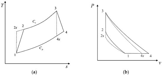
Figure 1. (a) $T-s$ representation of Atkinson cycle [62]. (b) $p-v$ representation of Atkinson cycle.

In the early research [62], the WF’s SHs were assumed to be constants, but in the actual cycle, accompanying with the combustion reaction, the nature and composition of WF will change. For this reason, the variable SH model can be used to obtain more accurate results. When the cycle-working-temperature range is $300\hspace{0.17em}\mathrm{K}-3500\hspace{0.17em}\mathrm{K}$, the nonlinear variable SH model is defined as [85]

$$\begin{array}{l}{C}_p=7.2674\times {10}^{-10}{T}^2+4.2166\times {10}^{-6}{T}^{1.5}-1.23134\times {10}^{-5}T+9.1698\times {10}^{-4}{T}^{0.5}\\ \hspace{1em}\hspace{1em}+ 38.5787-4.3848\times {10}^5{T}^{-1.5}+8.8827\times {10}^6{T}^{-2}-6.4148\times {10}^8{T}^{-3}\end{array}$$

(1)

According to the relationship between constant pressure SH and constant volume SH, one has

$$C_v=C_p-R$$

(2)

Then, the constant volume SH of the cycle is

$$\begin{array}{c}{C}_v=C_p-R=7.2674\times {10}^{-10}{T}^2+4.2166\times {10}^{-6}{T}^{1.5}-1.23134\times {10}^{-5}T+9.1698\times {10}^{-4}{T}^{0.5}\hfill \\ \hspace{1em}\hspace{1em}+ 30.2642-4.3848\times {10}^5{T}^{-1.5}+8.8827\times {10}^6{T}^{-2}-6.4148\times {10}^8{T}^{-3}\hfill \end{array}$$

(3)

where $R=8.3145\mathrm{J}/(\mathrm{mol}·\mathrm{K})$ is the WF’s gas constant.

The heat flux rate supplied to the AC is

$$\begin{array}{c}U=Q_{in}\hfill \\ \hspace{1em}=\dot{m}{\int }_{T_2}^{T_3}{C}_{v}dT=\dot{m}{\int }_{T_2}^{T_3}(7.2674\times {10}^{-10}{T}^2+4.2166\times {10}^{-6}{T}^{1.5}-1.23134\times {10}^{-5}T+9.1698\hfill \\ \hspace{1em}\hspace{1em}\times {10}^{-4}{T}^{0.5}+30.2642-4.3848\times {10}^5{T}^{-1.5}+8.8827\times {10}^6{T}^{-2}-6.4148\times {10}^8{T}^{-3})\hspace{0.17em}dT\hfill \\ \hspace{1em}=\dot{m}[2.422\times {10}^{-10}{T}^3+1.6866\times {10}^{-6}{T}^{2.5}-6.1567\times {10}^{-6}{T}^2+6.1132\times {10}^{-4}{T}^{1.5}+\hfill \\ \hspace{1em}\hspace{1em}30.2642T+8.7696\times {10}^5{T}^{-0.5}-8.8827\times {10}^6{T}^{-1}+3.2074\times {10}^8{T}^{-2}{]}_{T_2}^{T_3}\hfill \end{array}$$

(4)

where $\dot{m}$ is the molar flow rate of the WF.

The heat flux rate transferred to the environment is

$$\begin{array}{c}{Q}_{out}=-\dot{m}{\int }_{T_4}^{T_1}{C}_{p}dT=\dot{m}{\int }_{T_1}^{T_4}{C}_{p}dT\hfill \\ \hspace{1em}\hspace{1em}=\dot{m}{\int }_{T_1}^{T_4}(7.2674\times {10}^{-10}{T}^2+4.2166\times {10}^{-6}{T}^{1.5}-1.23134\times {10}^{-5}T+9.1698\hfill \\ \hspace{1em}\hspace{1em}\hspace{1em}\times {10}^{-4}{T}^{0.5}+38.5787-4.3848\times {10}^5{T}^{-1.5}+8.8827\times {10}^6{T}^{-2}-6.4148\times {10}^8{T}^{-3})\hspace{0.17em}dT\hfill \\ \hspace{1em}\hspace{1em}=\dot{m}[2.422\times {10}^{-10}{T}^3+1.6866\times {10}^{-6}{T}^{2.5}-3.0783\times {10}^{-6}{T}^2+6.1132\times {10}^{-4}{T}^{1.5}\hfill \\ \hspace{1em}\hspace{1em}\hspace{1em}+\hspace{0.17em}38.5787T+8.7696\times {10}^5{T}^{-0.5}-8.8827\times {10}^6{T}^{-1}+3.2074\times {10}^8{T}^{-2}{]}_{T_1}^{T_4}\hfill \end{array}$$

(5)

For the two irreversible adiabatic processes $1\to 2$ and $3\to 4$, the IIL is defined as the irreversible compression and expansion efficiencies [62,70]

$${\eta }_c=(T_{2s}-T_1)/(T_2-T_1)$$

(6)

$${\eta }_e=(T_4-T_3)/(T_{4s}-T_3)$$

(7)

According to reference [70], the adiabatic process can be decomposed into numerous infinitely small processes. It is approximately considered that each infinitely small process has a constant adiabatic index. When the temperature of the WF changes $dT$ and the specific volume changes $dV$, one has

$$T{V}^{k-1}={(V+dV)}^{k-1}(T+dT)$$

(8)

Changing Equation (8) one can obtain:

$$C_v\ln (T_i/T_j)=-R\ln (V_i/V_j)$$

(9)

where the temperature in $C_v$ is the logarithmic average temperature between states $i$ and $j$, and $T=(T_i-T_j)/\ln (T_i/T_j)$.

The cycle compression ratio $\gamma$ and maximum temperature ratio $\tau$ are defined as

$$\gamma =V_1/V_2$$

(10)

$$\tau =T_3/T_1$$

(11)

Therefore, for the two adiabatic processes $1\to 2\hspace{0.17em}s$ and $3\to 4\hspace{0.17em}s$ of an irreversible AC with WF’s SHs as nonlinear variable with its temperature, one has

$$C_v\ln (T_{2s}/T_1)=R\ln \gamma$$

(12)

$$C_v\ln (T_{4s}/T_3)-R\ln (T_1/T_{4s})=-R\ln \gamma$$

(13)

According to the reference [62], the HTL rate and the power loss due to FL are expressed as

$${\dot{Q}}_{leak}=B(T_2+T_3-2T_0)$$

(14)

$$P_{\mu }=d{W}_{\mu }/dt=-\mu {(dx/dt)}^2=-\mu v^2=b{(\gamma -1)}^2$$

(15)

where $b=\mu x_2^2/{(\Delta t_{12})}^2$, the heat transfer coefficient is expressed as $B$, the ambient temperature is expressed as $T_0$, the work consumed by friction loss is expressed as $W_{\mu }$, the friction coefficient is expressed as $\mu$, the piston position at the minimum volume is expressed as $x_2$, and the power stroke time is expressed as $\Delta t_{12}$.

The $P$ and $\eta$ of the AC are, respectively

$$\begin{array}{c}P=Q_{in}-Q_{out}-P_{\mu }\\ =\dot{m}[2.422\times {10}^{-10}(T_1^3+T_3^3-T_2^3-T_4^3)+1.6866\times {10}^{-6}(T_1^{2.5}+T_3^{2.5}-T_2^{2.5}-T_4^{2.5})-6.1567\times \hfill \\ {10}^{-6}(T_1^2+T_3^2-T_2^2-T_4^2)+6.1132\times {10}^{-4}(T_1^{1.5}+T_3^{1.5}-T_2^{1.5}-T_4^{1.5})+30.2642(T_3-T_2)-\hfill \\ 38.5787(T_4-T_1)+8.7696\times {10}^5(T_1^{-0.5}+T_3^{-0.5}-T_2^{-0.5}-T_4^{-0.5})-8.8827\times {10}^6(T_1^{-1}+T_3^{-1}-\hfill \\ T_2^{-1}-T_4^{-1})+3.2074\times {10}^8(T_1^{-2}+T_3^{-2}-T_2^{-2}-T_4^{-2})]-b(\gamma -1{)}^2\hfill \end{array}$$

(16)

$$\begin{gathered} \eta =P/(Q_{in}+Q_{leak}) \\ =\frac{\dot{m}[2.422\times {10}^{-10}(T_1^3+T_3^3-T_2^3-T_4^3)+1.6866\times {10}^{-6}(T_1^{2.5}+T_3^{2.5}-T_2^{2.5}-T_4^{2.5})-6.1567\times \\ {10}^{-6}(T_1^2+T_3^2-T_2^2-T_4^2)+6.1132\times {10}^{-4}(T_1^{1.5}+T_3^{1.5}-T_2^{1.5}-T_4^{1.5})+30.2642(T_3-T_2)- \\ 38.5787(T_4-T_1)+8.7696\times {10}^5(T_1^{-0.5}+T_3^{-0.5}-T_2^{-0.5}-T_4^{-0.5})-8.8827\times {10}^6(T_1^{-1}+T_3^{-1}- \\ {T}_2^{-1}-T_4^{-1})+3.2074\times {10}^8(T_1^{-2}+T_3^{-2}-T_2^{-2}-T_4^{-2})]-b(\gamma -1{)}^2}{\dot{m}[2.422\times {10}^{-10}(T_3^3-T_2^3)+1.6866\times {10}^{-6}(T_3^{2.5}-T_2^{2.5})-6.1567\times {10}^{-6}(T_3^2-T_2^2)+6.1132\times \\ {10}^{-4}(T_3^{1.5}-T_2^{1.5})+30.2642(T_3-T_2)+8.7696\times {10}^5(T_3^{-0.5}-T_2^{-0.5})-8.8827\times {10}^6(T_3^{-1}-T_2^{-1}) \\ +3.2074\times {10}^8(T_3^{-2}-T_2^{-2})]+B(T_2+T_3-2T_0)} \end{gathered}$$

(17)

According to the definition of $P_d$ in references [55,62], one has

$$P_d=P/v_{\max }=P/v_4$$

(18)

The entropy production rates resulting from the HTL, FL, and IIL are defined as

$${\sigma }_q=B(T_2+T_3-2T_0)[1/T_0-2/(T_2+T_3)]$$

(19)

$${\sigma }_{\mu }=P_{\mu }/T_0=b{(\gamma -1)}^2/T_0$$

(20)

$$\begin{array}{c}{\sigma }_{2s\to 2}=\dot{m}{\int }_{T_{2s}}^{T_2}{C}_{v}dT/T\\ \hspace{1em}=\dot{m}[3.6337\times {10}^{-10}(T_2^2-T_{2s}^2)+2.8111\times {10}^{-6}(T_2^{1.5}-T_{2s}^{1.5})-1.23134\times {10}^{-5}(T_2-T_{2s})\hfill \\ \hspace{1em}\hspace{1em}+1.8339\times {10}^{-3}(T_2^{0.5}-T_{2s}^{0.5})+30.2642\ln (T_2/T_{2s})+2.9232\times {10}^5(T_2^{-1.5}-T_{2s}^{-1.5})-\hfill \\ \hspace{1em}\hspace{1em}4.4413\times {10}^6(T_2^{-2}-T_{2s}^{-2})+2.1382\times {10}^8(T_2^{-3}-T_{2s}^{-3})]\hfill \end{array}$$

(21)

$$\begin{array}{c}{\sigma }_{4s\to 4}=\dot{m}{\int }_{T_{4s}}^{T_4}{C}_{p}dT/T\\ \hspace{1em}=\dot{m}[3.6337\times {10}^{-10}(T_4^2-T_{4s}^2)+2.8111\times {10}^{-6}(T_4^{1.5}-T_{4s}^{1.5})-1.23134\times {10}^{-5}(T_4-T_{4s})\hfill \\ \hspace{1em}\hspace{1em}+1.8339\times {10}^{-3}(T_4^{0.5}-T_{4s}^{0.5})+38.5787\ln (T_4/T_{4s})+2.9232\times {10}^5(T_4^{-1.5}-T_{4s}^{-1.5})-\hfill \\ \hspace{1em}\hspace{1em}4.4413\times {10}^6(T_4^{-2}-T_{4s}^{-2})+2.1382\times {10}^8(T_4^{-3}-T_{4s}^{-3})]\hfill \end{array}$$

(22)

The entropy production rate produced by the exhaust stroke is

$$\begin{array}{c}{\sigma }_{pq}=\dot{m}{\int }_{T_1}^{T_4}{C}_{p}dT(1/T_0-1/T)\\ \hspace{1em}=(\dot{m}/T_0)[2.422\times {10}^{-10}(T_4^3-T_1^3)+1.6866\times {10}^{-6}(T_4^{2.5}-T_1^{2.5})-6.1567\times {10}^{-6}(T_4^2-T_1^2)\hfill \\ \hspace{1em}\hspace{1em}+6.113\times {10}^{-4}(T_4^{1.5}-T_1^{1.5})+38.5787(T_4-T_1)+8.7696\times {10}^5(T_4^{-0.5}-T_1^{-0.5})-8.8827\hfill \\ \hspace{1em}\hspace{1em}\times {10}^6(T_4^{-1}-T_1^{-1})+3.2074\times {10}^8(T_4^{-2}-T_1^{-2})]-\dot{m}[3.6337\times {10}^{-10}(T_4^2-T_1^2)+2.8111\times \hfill \\ \hspace{1em}\hspace{1em}{10}^{-6}(T_4^{1.5}-T_1^{1.5})-1.2313\times {10}^{-5}(T_4-T_1)+1.8339\times {10}^{-3}(T_4^{0.5}-T_1^{0.5})+38.5787\ln (T_4\hfill \\ \hspace{1em}\hspace{1em}/T_1)+2.9232\times {10}^5(T_4^{-1.5}-T_1^{-1.5})-4.4413\times {10}^6(T_4^{-2}-T_1^{-2})+2.1382\times {10}^8(T_4^{-3}-T_1^{-3})]\hfill \end{array}$$

(23)

The total entropy production rate due to HTL, FL, IIL and exhaust process is

$$\begin{array}{c}\sigma ={\sigma }_q+{\sigma }_{\mu }+{\sigma }_{2s\to 2}+{\sigma }_{4s\to 4}+{\sigma }_{pq}\\ \hspace{1em}=B_1(T_2+T_3-2T_0)[(1/T_0)-2/(T_2+T_3)]+b(\gamma -1{)}^2/T_0+\dot{m}[3.6337\times {10}^{-10}(T_2^2-T_{2s}{}^2-T_{4s}^2+\hfill \\ \hspace{1em}\hspace{1em}{T}_1^2)+2.8111\times {10}^{-6}(T_2^{1.5}-T_{2s}^{1.5}-T_{4s}^{1.5}+T_1^{1.5})-1.23134\times {10}^{-5}(T_2-T_{2s}-T_{4s}+T_1)+1.8339\hfill \\ \hspace{1em}\hspace{1em}\times {10}^{-3}(T_2^{0.5}-T_{2s}^{0.5}-T_{4s}^{0.5}+T_1^{0.5})+30.2642\ln (T_2/T_{2s})-38.5787\ln (T_{4s}/T_1)+2.9232\times {10}^5\hfill \\ \hspace{1em}\hspace{1em}(T_2^{-1.5}-T_{2s}^{-1.5}-T_{4s}^{-1.5}+T_1^{-1.5})-4.4413\times {10}^6(T_2^{-2}-T_{2s}^{-2}-T_{4s}^{-2}+T_1^{-2})+2.1382\times {10}^8(T_2^{-3}-\hfill \\ \hspace{1em}\hspace{1em}{T}_{2s}^{-3}-T_{4s}^{-3}+T_1^{-3})]+(\dot{m}/T_0)[2.422\times {10}^{-10}(T_4^3-T_1^3)+1.6866\times {10}^{-6}(T_4^{2.5}-T_1^{2.5})-6.1567\times \hfill \\ \hspace{1em}\hspace{1em}{10}^{-6}(T_4^2-T_1^2)+6.1132\times {10}^{-4}(T_4^{1.5}-T_1^{1.5})+38.5787(T_4-T_1)+8.7696\times {10}^5(T_4^{-0.5}-T_1^{-0.5})\hfill \\ \hspace{1em}\hspace{1em}-8.8827\times {10}^6(T_4^{-1}-T_1^{-1})+3.2074\times {10}^8(T_4^{-2}-T_1^{-2})]\hfill \end{array}$$

(24)

According to the definition of $E$ in references [96,97,98], one has

$$\begin{array}{c}E=P-T_0\sigma \\ \hspace{1em}=\dot{m}[2.422\times {10}^{-10}(T_3^3+2T_1^3-T_2^3-2T_4^3)+1.6866\times {10}^{-6}(T_3^{2.5}+2T_1^{2.5}-T_2^{2.5}-2T_4^{2.5})-6.1567\hfill \\ \hspace{1em}\hspace{1em}\times {10}^{-6}(T_3^2+2T_1^2-T_2^2-2T_4^2)+6.1132\times {10}^{-4}(T_3^{1.5}+2T_1^{1.5}-T_2^{1.5}-2T_4^{1.5})+30.2642(T_3-T_2)\hfill \\ \hspace{1em}\hspace{1em}-38.5787(2T_4-2T_1)+8.7696\times {10}^5(T_3^{-0.5}+2T_1^{-0.5}-T_2^{-0.5}-2T_4^{-0.5})-8.8827\times {10}^6(T_3^{-1}+\hfill \\ \hspace{1em}\hspace{1em}2T_1^{-1}-T_2^{-1}-2T_4^{-1})+3.2074\times {10}^8(T_3^{-2}+2T_1^{-2}-T_2^{-2}-2T_4^{-2})]-\dot{m}{T}_0[3.6337\times {10}^{-10}(T_2^2-T_{2s}^2\hfill \\ \hspace{1em}\hspace{1em}-T_{4s}^2+T_1^2)+2.8111\times {10}^{-6}(T_2^{1.5}-T_{2s}^{1.5}-T_{4s}^{1.5}+T_1^{1.5})-1.23134\times {10}^{-5}(T_2-T_{2s}-T_{4s}+T_1)+\hfill \\ \hspace{1em}\hspace{1em}1.8339\times {10}^{-3}(T_2^{0.5}-T_{2s}^{0.5}-T_{4s}^{0.5}+T_1^{0.5})+30.2642\ln (T_2/T_{2s})-38.5787\ln (T_{4s}/T_1)+2.9232\hfill \\ \hspace{1em}\hspace{1em}\times {10}^5(T_2^{-1.5}-T_{2s}^{-1.5}-T_{4s}^{-1.5}+T_1^{-1.5})-4.4413\times {10}^6(T_2^{-2}-T_{2s}^{-2}-T_{4s}^{-2}+T_1^{-2})+2.1382\times {10}^8(T_2^{-3}\hfill \\ \hspace{1em}\hspace{1em}-T_{2s}^{-3}-T_{4s}^{-3}+T_1^{-3})]-B_1(T_2+T_3-2T_0)[1-2T_0/(T_2+T_3)]-2b(\gamma -1{)}^2\hfill \end{array}$$

(25)

According to the treatment method in the references [55,62], the $\overline{P}$, $\eta$, $\overline{E}$, and ${\overline{P}}_d$ are defined as

$$\overline{P}=P/P_{\max }$$

(26)

$${\overline{P}}_d=P_d/{(P_d)}_{\max }$$

(27)

$$\overline{E}=E/E_{\max }$$

(28)

When the compression ratio $\gamma$, the cycle initial temperature $T_1$, and the maximum temperature ratio $\tau$ are given, the numerical solutions of temperatures at each state point and cycle performances can be obtained.

3. Performance Optimization with the Maximum Power Density Criterion

According to reference [62], the values of the cycle parameters can be determined: $\dot{m}=1\hspace{0.17em}\mathrm{mol}/\mathrm{s}$, $T_0=300\hspace{0.17em}\mathrm{K}$, $T_1=350\hspace{0.17em}\mathrm{K}$, $B=2.2\hspace{0.17em}\mathrm{W}\mathrm{/}\mathrm{K}$, $\tau =4.28-6.28$, $b=20\hspace{0.17em}\mathrm{W}$.

Figure 2 and Figure 3 show the effect of cycle maximum temperature ratio ($\tau$) on cycle dimensionless power density versus compression ratio (${\overline{P}}_d-\gamma$) and cycle dimensionless power density versus thermal efficiency (${\overline{P}}_d-\eta$), respectively. It can be noticed that there is an optimal compression ratio (${\gamma }_{{\overline{P}}_d}$) to make ${\overline{P}}_d$ reach the maximum. As the $\tau$ increases from 5.78 to 6.78, the ${\gamma }_{{\overline{P}}_d}$ increases from 8.3 to 9.0, and increases by about 8.434%. The ${\eta }_{{\overline{P}}_d}$ corresponding to the cycle maximum ${\overline{P}}_d$ increases from 0.4330 to 0.4579, and increases by 5.75%. It shows that under the maximum $P_d$ criterion, the increases of the ${\gamma }_{{\overline{P}}_d}$ and ${\eta }_{{\overline{P}}_d}$ of the cycle are accompanied with the increase of the $\tau$.

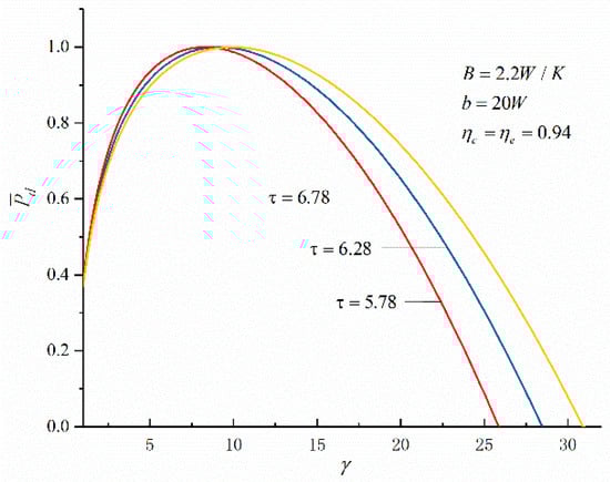
Figure 2. The curves of ${\overline{P}}_d-\gamma$ about $\tau$.

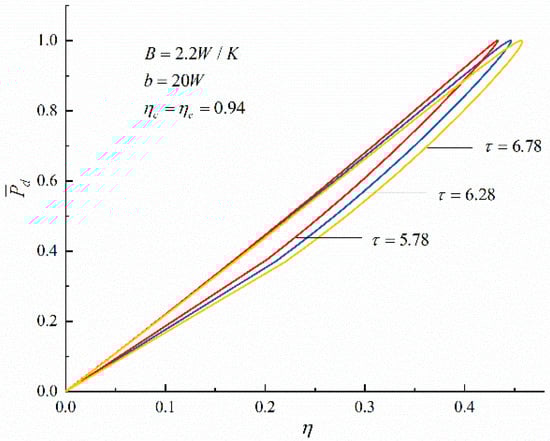
Figure 3. The curves of ${\overline{P}}_d-\eta$ about $\tau$.

Figure 4 and Figure 5 show the characteristic relationships of ${\overline{P}}_d-\gamma$ and ${\overline{P}}_d-\eta$ with different loss combinations. In Figure 4, when only considering the FL, comparing curves $1$ and $2$, the FL increases from $0$ to $20\hspace{0.17em}\mathrm{W}$, the ${\gamma }_{{\overline{P}}_d}$ will decrease from 31.4 to 10.9 and decrease by 65.287%. When only considering the IIL, comparing curves $1$ and $1^{\prime }$, the IIL increases (from 1 to 0.94), the ${\gamma }_{{\overline{P}}_d}$ will decrease from 31.4 to 18.5, and decrease by 41.083%. When considering both FL and IIL, comparing curves $1$ and $2^{\prime }$, the IIL increases (from 1 to 0.94) the FL increases from $0$ to $20\hspace{0.17em}\mathrm{W}$, the ${\gamma }_{{\overline{P}}_d}$ will decrease from 31.4 to 9.1 and decrease by 71.019%. It can be seen that the decrease of the ${\gamma }_{{\overline{P}}_d}$ of the cycle is accompanied with the increases of the cycle losses.

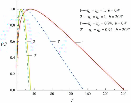
Figure 4. The curves of ${\overline{P}}_d-\gamma$ about ${\eta }_c$, ${\eta }_e$, and $b$.

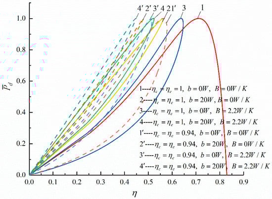
Figure 5. The curves of ${\overline{P}}_d-\eta$ about ${\eta }_c$, ${\eta }_e$, $B$, and $b$.

In Figure 5, when only considering the FL, comparing curves $1$ and $2$, the FL increases from $0$ to $20\hspace{0.17em}\mathrm{W}$, the ${\eta }_{{\overline{P}}_d}$ will decrease from 0.7114 to 0.5611 and decrease by 21.13%. When only considering the HTL, comparing curves $1$ and $3$, the HTL increases from $0$ to $2.2\hspace{0.17em}\mathrm{W}\mathrm{/}\mathrm{K}$, the ${\eta }_{{\overline{P}}_d}$ will decrease from 0.7114 to 0.6371 and decrease by 10.44%. When only considering the IIL, comparing curves $1$ and $1^{\prime }$, the IIL increases (from 1 to 0.94), the ${\eta }_{{\overline{P}}_d}$ will decrease from 0.7114 to 0.5618 and decrease by 21.03%. When considering HTL and FL at the same time, comparing curves $1$ and $4$, the HTL increases from $0$ to $2.2\hspace{0.17em}\mathrm{W}\mathrm{/}\mathrm{K}$ and the FL increases from $0$ to $20\hspace{0.17em}\mathrm{W}$, the ${\eta }_{{\overline{P}}_d}$ will decrease from 0.7114 to 0.5213 and decrease by 23.72%. When considering HTL and IIL, comparing curves $1$ and $3^{\prime }$, the HTL increases from $0$ to $2.2\hspace{0.17em}\mathrm{W}\mathrm{/}\mathrm{K}$ and the IIL increases (from 1 to 0.94), the ${\eta }_{{\overline{P}}_d}$ will decrease from 0.7114 to 0.5122 and decrease by 28.00%. When considering FL and IIL, comparing curves $1$ and $2^{\prime }$, the FL increases from $0$ to $20\hspace{0.17em}\mathrm{W}$ and the IIL increases (from 1 to 0.94), the ${\eta }_{{\overline{P}}_d}$ will decrease from 0.7114 to 0.4791 and decrease by 32.65%. When considering FL, HTL, and IIL at the same time, comparing curves $1$ and $4^{\prime }$, the FL increases from $0$ to $20\hspace{0.17em}\mathrm{W}$, the HTL increases from $0$ to $2.2\hspace{0.17em}\mathrm{W}\mathrm{/}\mathrm{K}$, and the IIL increases from 1 to 0.94, the ${\eta }_{{\overline{P}}_d}$ will decrease from 0.7114 to 0.4459 and decrease by 37.32%. It can be seen that the decrease of the ${\eta }_{{\overline{P}}_d}$ of the cycle is accompanied with the increases of the cycle losses.

Figure 6, Figure 7 and Figure 8 show the compared results of the cycle $\eta$, maximum specific volume ratio, and pressure ratio under the maximum $P$ and maximum $P_d$ criterions when there are three losses. Comparing with the maximum $P$ criterion, the $\eta$ and maximum pressure ratio under the maximum $P_d$ criterion are higher, while the maximum specific volume ratio under the maximum $P_d$ criterion is smaller. Therefore, the engine designed based on the maximum $P_d$ criterion is smaller in size and more efficient.

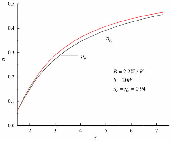
Figure 6. The curves of $\eta$ versus $\tau$.

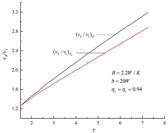
Figure 7. The curves of $v_4/v_1$ versus $\tau$.

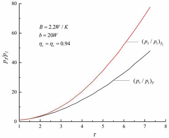
Figure 8. The curves of $p_3/p_1$ versus $\tau$.

4. Multi-Objective Optimization

In actual cycle, there is no point at which the $P$, $\eta$, $E$, and $P_d$ are optimized at the same time. Therefore, when solving the MOO problem, it is very important to take into account the trade-offs between the interests of different objectives, and obtain the Pareto optimal solution that simultaneously satisfies multiple different or even contradictory goals. The Pareto frontier is defined as the solution set of the optimization objectives. Figure 9 shows the algorithm diagram of NSGA-II [62]. When taking the compression ratio as the optimization variable and taking the $\overline{P}$, $\eta$, $\overline{E}$, and ${\overline{P}}_d$ as the optimization objectives, the single-, bi-, tri-, and quadru-objective optimization results are obtained. The optimal solution is obtained by comparing the magnitude of the deviation indexes obtained by LINMAP, TOPSIS, and Shannon entropy solutions.

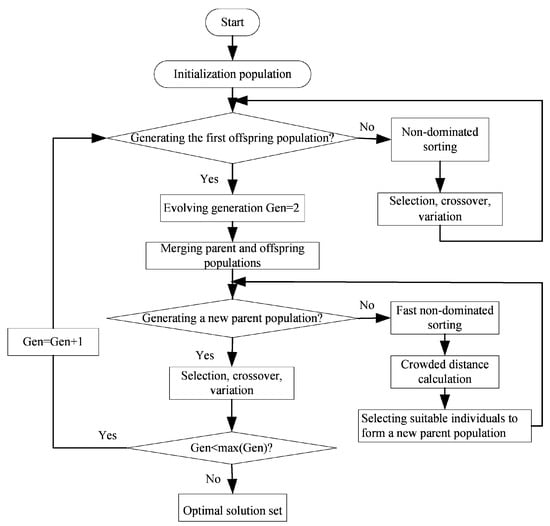
Figure 9. Flow chart of NSGA-II [62].

The optimization problems are solved with different optimization objective combinations, which forms different MOO problems. The one quadru-objective optimization problem is as follows:

$$\max \left\{\begin{array}{l}{\overline{P}}_d(\gamma )\\ \eta (\gamma )\\ \overline{E}(\gamma )\\ {\overline{P}}_d(\gamma )\end{array}\right.$$

(29)

The four tri-objective optimization problems are as follows:

$$\max \left\{\begin{array}{l}\overline{P}(\gamma )\\ \eta (\gamma )\\ \overline{E}(\gamma )\end{array}\right.,\max \left\{\begin{array}{l}\overline{P}(\gamma )\\ \eta (\gamma )\\ {\overline{P}}_d(\gamma )\end{array}\right.,\max \left\{\begin{array}{l}\overline{P}(\gamma )\\ \overline{E}(\gamma )\\ {\overline{P}}_d(\gamma )\end{array}\right.,\max \left\{\begin{array}{l}\eta (\gamma )\\ \overline{E}(\gamma )\\ {\overline{P}}_d(\gamma )\end{array}\right.$$

(30)

The six bi-objective optimization problems are as follows:

$$\max \left\{\begin{array}{l}\overline{P}(\gamma )\\ \eta (\gamma )\end{array}\right.,\max \left\{\begin{array}{l}\overline{P}(\gamma )\\ \overline{E}(\gamma )\end{array}\right.,\max \left\{\begin{array}{l}\overline{P}(\gamma )\\ {\overline{P}}_d(\gamma )\end{array}\right.,\max \left\{\begin{array}{l}\eta (\gamma )\\ \overline{E}(\gamma )\end{array}\right.,\max \left\{\begin{array}{l}\eta (\gamma )\\ {\overline{P}}_d(\gamma )\end{array}\right.,\max \left\{\begin{array}{l}\overline{E}(\gamma )\\ {\overline{P}}_d(\gamma )\end{array}\right.$$

(31)

Table 1 lists the results of the MOO based on LINMAP, TOPSIS, and Shannon entropy solutions under different combinations of optimization objectives, and lists the results of single-objective optimization corresponding to the maximum $\overline{P}$, maximum $\eta$, maximum $\overline{E}$, and maximum ${\overline{P}}_d$, and the corresponding deviation index. Figure 10, Figure 11, Figure 12, Figure 13, Figure 14, Figure 15, Figure 16, Figure 17, Figure 18, Figure 19 and Figure 20 show the Pareto frontiers of different combinations of single-, bi-, tri-, and quadru-objective optimizations. The diamond represents the corresponding points of Shannon entropy solution, and the positive and negative triangles represent the corresponding points of LINMAP and TOPSIS solutions, respectively.

Table 1. Outcomes of decision-making methods for MOO and single-objective optimizations.

Optimization Methods	Decision Methods	Optimization Variable	Optimization Objectives				Deviation Index
		$\mathit{\gamma }$	$\overline{\mathit{P}}$	$\mathit{\eta }$	$\overline{\mathit{E}}$	${\overline{\mathit{P}}}_{\mathit{d}}$	$\mathit{D}$
Quadru-objective optimization ($\overline{P}$, $\eta$, $\overline{E}$ and ${\overline{P}}_d$)	LINMAP	7.5172	0.9865	0.4450	0.9997	0.9890	0.1250
	TOPSIS	7.5172	0.9865	0.4450	0.9997	0.9890	0.1250
	Shannon Entropy	9.1311	0.9564	0.4459	0.9345	0.9999	0.5266
Tri-objective optimization ($\overline{P}$, $\eta$ and $\overline{E}$)	LINMAP	7.1952	0.9907	0.4438	0.9958	0.9839	0.1395
	TOPSIS	7.2939	0.9895	0.4442	0.9978	0.9856	0.1307
	Shannon Entropy	7.5582	0.9859	0.4451	0.9998	0.9896	0.1253
Tri-objective optimization ($\overline{P}$, $\eta$ and ${\overline{P}}_d$)	LINMAP	7.5054	0.9866	0.4449	0.9999	0.9888	0.1247
	TOPSIS	7.5485	0.9860	0.4451	0.9999	0.9894	0.1252
	Shannon Entropy	9.1297	0.9564	0.4459	0.9349	0.9999	0.5247
Tri-objective optimization ($\overline{P}$, $\overline{E}$ and ${\overline{P}}_d$)	LINMAP	7.4763	0.9871	0.4449	0.9996	0.9883	0.1249
	TOPSIS	7.4763	0.9871	0.4449	0.9996	0.9883	0.1249
	Shannon Entropy	9.1314	0.9564	0.4459	0.9345	0.9999	0.5279
Tri-objective optimization ($\eta$, $\overline{E}$ and ${\overline{P}}_d$)	LINMAP	7.8916	0.9808	0.4459	0.9966	0.9936	0.1457
	TOPSIS	7.8817	0.9809	0.4459	0.9968	0.9935	0.1450
	Shannon Entropy	9.1320	0.4459	0.9344	0.9345	0.9999	0.5269
Bi-objective optimization ($\overline{P}$ and $\eta$)	LINMAP	7.0477	0.9924	0.4431	0.9920	0.9812	0.1609
	TOPSIS	7.0330	0.9926	0.4431	0.9915	0.9809	0.1639
	Shannon Entropy	8.4845	0.9700	0.4465	0.9764	0.9983	0.2074
Bi-objective optimization ($\overline{P}$ and $\overline{E}$)	LINMAP	7.1705	0.9910	0.4437	0.9952	0.9835	0.1423
	TOPSIS	7.1705	0.9910	0.4437	0.9952	0.9835	0.1423
	Shannon Entropy	7.5573	0.9859	0.4451	0.9998	0.9896	0.1252
Bi-objective optimization ($\overline{P}$ and ${\overline{P}}_d$)	LINMAP	7.4628	0.9872	0.4448	0.9980	0.9882	0.1248
	TOPSIS	7.5003	0.9867	0.4450	0.9999	0.9887	0.1248
	Shannon Entropy	9.1277	0.9564	0.4459	0.9350	0.9999	0.5241
Bi-objective optimization ($\eta$ and $\overline{E}$)	LINMAP	7.7359	0.9832	0.4456	0.9989	0.9919	0.1328
	TOPSIS	7.7259	0.9834	0.4456	0.9990	0.9918	0.1318
	Shannon Entropy	7.5597	0.9859	0.4451	0.9998	0.9896	0.1252
Bi-objective optimization ($\eta$ and ${\overline{P}}_d$)	LINMAP	8.8286	0.9630	0.4463	0.9566	0.9996	0.3968
	TOPSIS	8.8388	0.9628	0.4463	0.9559	0.9996	0.4011
	Shannon Entropy	9.1297	0.9564	0.4459	0.9349	0.9999	0.5247
Bi-objective optimization ($\overline{E}$ and ${\overline{P}}_d$)	LINMAP	7.8949	0.9807	0.4460	0.9965	0.9936	0.1463
	TOPSIS	7.8857	0.9813	0.4459	0.9967	0.9935	0.1427
	Shannon Entropy	9.1334	0.9563	0.4459	0.9999	0.9999	0.5276
Maximum of $\overline{P}$	——	5.8100	0.9999	0.4338	0.8928	0.9478	0.7326
Maximum of $\eta$	——	8.5000	0.9697	0.4465	0.9756	0.9984	0.2752
Maximum of $\overline{E}$	——	7.5900	0.9853	0.4453	0.9998	0.9902	0.1260
Maximum of ${\overline{P}}_d$	——	9.1300	0.9571	0.4459	0.9372	0.9999	0.5120
Positive ideal point		——	0.9999	0.4465	0.9998	0.9999	——
Negative ideal point		——	0.9564	0.4335	0.8895	0.9470	——

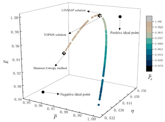
Figure 10. Quadru-objective optimization on $\overline{P}-\eta -\overline{E}-{\overline{P}}_d$.

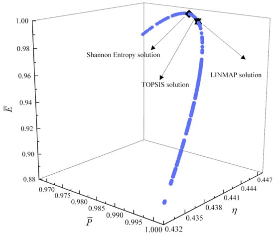
Figure 11. Tri-objective optimization on $\overline{P}-\eta -\overline{E}$.

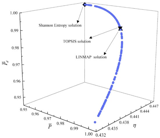
Figure 12. Tri-objective optimization on $\overline{P}-\eta -{\overline{P}}_d$.

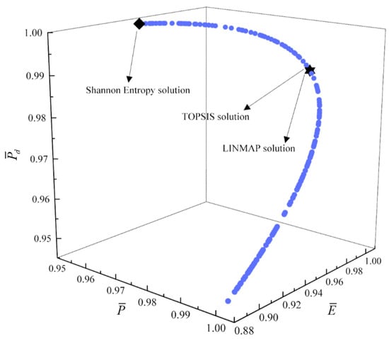
Figure 13. Tri-objective optimization on $\overline{P}-\overline{E}-{\overline{P}}_d$.

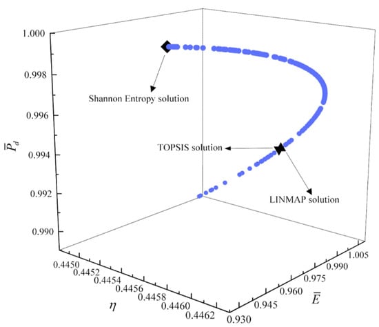
Figure 14. Tri-objective optimization on $\eta -\overline{E}-{\overline{P}}_d$.

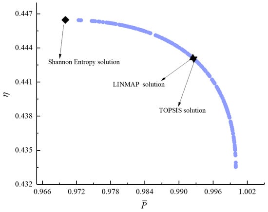
Figure 15. Bi-objective optimization on $\overline{P}-\eta$.

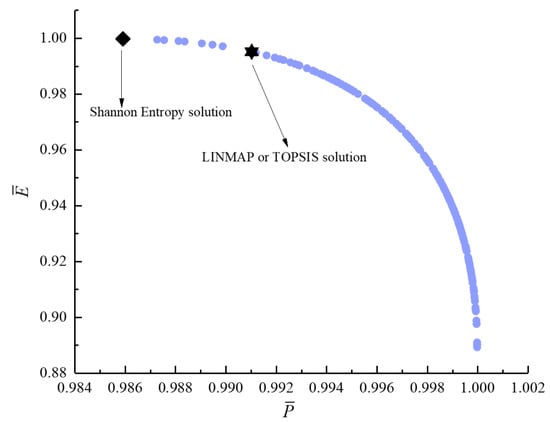
Figure 16. Bi-objective optimization on $\overline{P}-\overline{\underset{\dot{}}{E}}$.

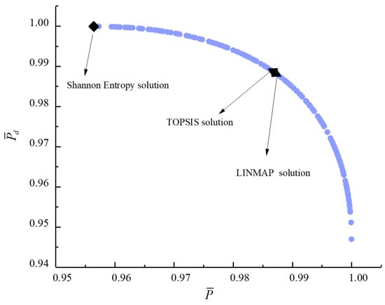
Figure 17. Bi-objective optimization on $\overline{P}-{\overline{P}}_d$.

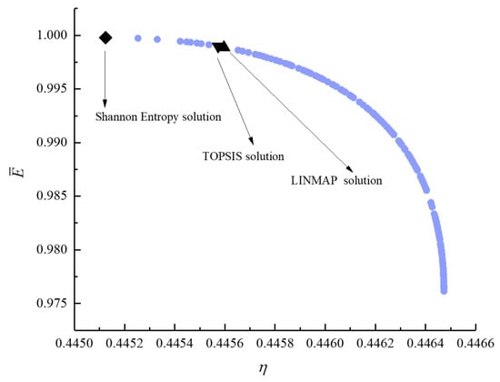
Figure 18. Bi-objective optimization on $\eta -\overline{\underset{\dot{}}{E}}$.

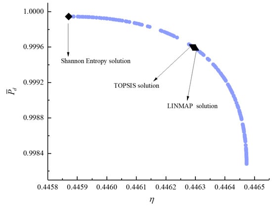
Figure 19. Bi-objective optimization on $\eta -{\overline{P}}_d$.

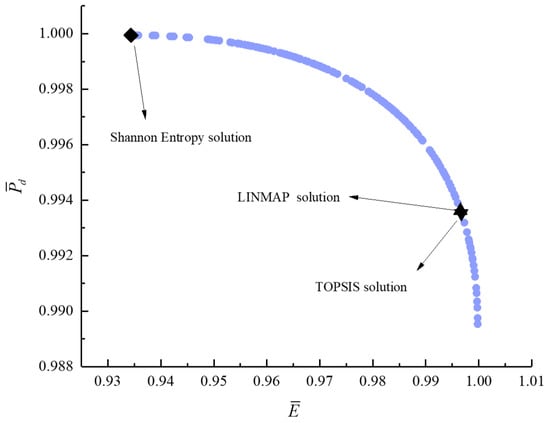
Figure 20. Bi-objective optimization on $\overline{E}-{\overline{P}}_d$.

The deviation indexes of maximum $\overline{P}$, maximum $\eta$, maximum $\overline{E}$, and maximum ${\overline{P}}_d$ are 0.7326, 0.2752, 0.1260, and 0.5120, respectively. For the quadrur-objective optimization, Figure 10 shows the Pareto frontier for $\overline{P}-\eta -\overline{E}-{\overline{P}}_d$. It can be noticed that with the increase of $\eta$, the $\overline{P}$ and ${\overline{P}}_d$ increase, and the $\overline{E}$ first increases and then decreases. The deviation indexes (0.1250, 0.1250, 0.5266) obtained by the LINMAP, TOPSIS, and Shannon entropy solutions are smaller than those of single-objective optimization. It means that the results obtained by four-objective optimization are more perfect than single-objective optimization. In addition, when taking $\overline{P}$, $\eta$, $\overline{E}$, and ${\overline{P}}_d$ as the objective functions, the deviation indexes obtained by LINMAP and TOPSIS solutions are the same, and the optimization results are more desirable than those obtained by the Shannon entropy solution.

For tri-objective optimization, Figure 11, Figure 12, Figure 13 and Figure 14 show the Pareto frontiers for $\overline{P}-\eta -\overline{E}$, $\overline{P}-\eta -{\overline{P}}_d$, $\overline{P}-\overline{E}-{\overline{P}}_d$, and $\eta -\overline{E}-{\overline{P}}_d$. It can be noticed that with the increases of $\eta$, the $\overline{P}$ and ${\overline{P}}_d$ increase, while the $\overline{E}$ first increases and then decreases. With the increase of ${\overline{P}}_d$, the $\overline{P}$ decreases, the $\eta$ increases, and the $\overline{E}$ first increases and then decreases. The deviation indexes obtained by different decision-makings are smaller than those obtained by single-objective optimization, and which is the same as that obtained by quadru-objective optimization. When taking $\overline{P}$, $\eta$, and $\overline{E}$ as the objective functions, the deviation index obtained by the Shannon entropy solution is smaller. When taking $\overline{P}$, $\eta$, and ${\overline{P}}_d$ as the objective functions, the deviation index obtained by the LINMAP solution is smaller. When taking $\overline{P}$, $\overline{E}$, and ${\overline{P}}_d$ as the objective functions, the LINMAP and TOPSIS solutions get the same deviation indexes, and the optimization results are more desirable than those obtained by the Shannon entropy solution. When taking $\eta$, $\overline{E}$, and ${\overline{P}}_d$ as the objective functions, the deviation index obtained by the TOPSIS solution is smaller and the result is better.

For bi-objective optimization, Figure 15, Figure 16, Figure 17, Figure 18, Figure 19 and Figure 20 show the Pareto frontiers for $\overline{P}-\eta$, $\overline{P}-\overline{\underset{\dot{}}{E}}$, $\overline{P}-{\overline{P}}_d$, $\eta -\overline{\underset{\dot{}}{E}}$, $\eta -{\overline{P}}_d$, and $\overline{E}-{\overline{P}}_d$. It can be noticed that the $\eta$, $\overline{E}$, and ${\overline{P}}_d$ decrease with the increase of $\overline{P}$, the $\overline{E}$ and ${\overline{P}}_d$ decrease with the increase of $\eta$, and the ${\overline{P}}_d$ decreases with the increase of $\overline{E}$. The indexes obtained by different decision-makings are smaller than those obtained by single-objective optimization, and the conclusion is the same as that obtained by tri- and quadru-objective optimization. When taking $\overline{P}$ and $\eta$ or taking ${\overline{P}}_d$ and $\eta$ as the objective functions, the deviation index obtained by the LINMAP solution is smaller. When taking $\overline{P}$ and $\overline{E}$ or taking $\eta$ and $\overline{E}$ as the objective functions, the deviation index obtained by the Shannon entropy solution is smaller. When taking $\overline{P}$ and ${\overline{P}}_d$ or taking $\overline{E}$ and ${\overline{P}}_d$ as the objective functions, the deviation index obtained by the TOPSIS solution is smaller and the result is better.

By comparing the deviation indexes obtained under various conditions, the results show that the solution obtained by MOO is more desirable, and the deviation indexes are smaller. In addition, when the LINMAP solution is optimized with $\overline{P}$, $\eta$, and ${\overline{P}}_d$ as the objective functions, the deviation index is 0.1247, the contradiction obtained is the smallest, and the result is the best. In practical applications, the optimal plan can be selected from the Pareto frontier, and the design can be optimized according to the actual requirements of the decision-maker.

5. Conclusions

Through FTT analysis, this paper performs the performance analyses of the irreversible AC under the maximum $P_d$ criterion when the WF’s SHs are nonlinear variable with its temperature. The results of the $\eta$, maximum specific volume ratio and pressure ratio obtained under the maximum $P_d$ criterion are compared with those under the maximum $P$ criterion. Based on NSGA-II, when the compression ratio is the optimization variable and the $\overline{P}$, $\eta$, $\overline{E}$, and ${\overline{P}}_d$ are the optimization objectives, the single-, bi-, tri-, and quadru-objective optimization results are obtained. The optimal solution is obtained by comparing the deviation indexes of LINMAP, TOPSIS, and Shannon entropy solutions. It can be noticed that:

(1)

There is an ${\gamma }_{{\overline{P}}_d}$ to maximize the ${\overline{P}}_d$. With the cycle maximum temperature ratio increases, the ${\gamma }_{{\overline{P}}_d}$ and ${\eta }_{{\overline{P}}_d}$ corresponding to the ${\overline{P}}_d$ will increase. With the increases of HTL, FL, IIL, the ${\gamma }_{{\overline{P}}_d}$ and ${\eta }_{{\overline{P}}_d}$ corresponding to the cycle maximum ${\overline{P}}_d$ will decrease.

(2)

Under the maximum $P_d$ criterion, the $\eta$ will be higher and the size will be smaller.

(3)

Compared with single-objective optimization, MOO has less contradictions and conflicts. Comparing the results of single-, bi-, tri-, and quadru-objective optimization, when the LINMAP solution is optimized with $\overline{P}$, $\eta$, and ${\overline{P}}_d$ as the objective functions, the contradiction is smaller and the result is more perfect.

References

- Andresen, B.; Berry, R.S.; Ondrechen, M.J.; Salamon, P. Thermodynamics for processes in finite time. Acc. Chem. Res. 1984, 17, 266–271. [Google Scholar] [CrossRef]
- Chen, L.G.; Wu, C.; Sun, F.R. Finite Time Thermodynamic Optimization or Entropy Generation Minimization of Energy Systems. J. Non-Equilib. Thermodyn. 1999, 22, 327–359. [Google Scholar] [CrossRef]
- Andresen, B. Current Trends in Finite-Time Thermodynamics. Angew. Chem. Int. Ed. 2011, 50, 2690–2704. [Google Scholar] [CrossRef] [PubMed]
- Berry, R.S.; Salamon, P.; Andresen, B. How It All Began. Entropy 2020, 22, 908. [Google Scholar] [CrossRef] [PubMed]
- Hoffmann, K.H.; Burzler, J.; Fischer, A.; Schaller, M.; Schubert, S. Optimal Process Paths for Endoreversible Systems. J. Non-Equilib. Thermodyn. 2003, 28, 233–268. [Google Scholar] [CrossRef]
- Zaeva, M.A.; Tsirlin, A.M.; Didina, O.V. Finite Time Thermodynamics: Realizability Domain of Heat to Work Converters. J. Non-Equilib. Thermodyn. 2019, 44, 181–191. [Google Scholar] [CrossRef]
- Masser, R.; Hoffmann, K.H. Endoreversible Modeling of a Hydraulic Recuperation System. Entropy 2020, 22, 383. [Google Scholar] [CrossRef] [PubMed] [Green Version]
- Kushner, A.; Lychagin, V.; Roop, M. Optimal Thermodynamic Processes for Gases. Entropy 2020, 22, 448. [Google Scholar] [CrossRef]
- De Vos, A. Endoreversible models for the thermodynamics of computing. Entropy 2020, 22, 660. [Google Scholar] [CrossRef]
- Masser, R.; Khodja, A.; Scheunert, M.; Schwalbe, K.; Fischer, A.; Paul, R.; Hoffmann, K.H. Optimized Piston Motion for an Alpha-Type Stirling Engine. Entropy 2020, 22, 700. [Google Scholar] [CrossRef]
- Chen, L.; Ma, K.; Ge, Y.; Feng, H. Re-Optimization of Expansion Work of a Heated Working Fluid with Generalized Radiative Heat Transfer Law. Entropy 2020, 22, 720. [Google Scholar] [CrossRef]
- Tsirlin, A.; Gagarina, L. Finite-Time Thermodynamics in Economics. Entropy 2020, 22, 891. [Google Scholar] [CrossRef]
- Tsirlin, A.; Sukin, I. Averaged Optimization and Finite-Time Thermodynamics. Entropy 2020, 22, 912. [Google Scholar] [CrossRef]
- Muschik, W.; Hoffmann, K.H. Modeling, Simulation, and Reconstruction of 2-Reservoir Heat-to-Power Processes in Finite-Time Thermodynamics. Entropy 2020, 22, 997. [Google Scholar] [CrossRef]
- Insinga, A.R. The Quantum Friction and Optimal Finite-Time Performance of the Quantum Otto Cycle. Entropy 2020, 22, 1060. [Google Scholar] [CrossRef]
- Schön, J.C. Optimal Control of Hydrogen Atom-Like Systems as Thermodynamic Engines in Finite Time. Entropy 2020, 22, 1066. [Google Scholar] [CrossRef]
- Andresen, B.; Essex, C. Thermodynamics at Very Long Time and Space Scales. Entropy 2020, 22, 1090. [Google Scholar] [CrossRef]
- Chen, L.; Ma, K.; Feng, H.; Ge, Y. Optimal Configuration of a Gas Expansion Process in a Piston-Type Cylinder with Generalized Convective Heat Transfer Law. Energies 2020, 13, 3229. [Google Scholar] [CrossRef]
- Scheunert, M.; Masser, R.; Khodja, A.; Paul, R.; Schwalbe, K.; Fischer, A.; Hoffmann, K.H. Power-Optimized Sinusoidal Piston Motion and Its Performance Gain for an Alpha-Type Stirling Engine with Limited Regeneration. Energies 2020, 13, 4564. [Google Scholar] [CrossRef]
- Boykov, S.; Andresen, B.; Akhremenkov, A.A.; Tsirlin, A.M. Evaluation of Irreversibility and Optimal Organization of an Integrated Multi-Stream Heat Exchange System. J. Non-Equilib. Thermodyn. 2020, 45, 155–171. [Google Scholar] [CrossRef]
- Chen, L.G.; Feng, H.J.; Ge, Y.L. Maximum energy output chemical pump configuration with an infinite-low- and a finite-high-chemical potential mass reservoirs. Energy Convers. Manag. 2020, 223, 113261. [Google Scholar] [CrossRef]
- Hoffmann, K.H.; Burzler, J.M.; Schubert, S. Endoreversible thermodynamics. J. Non-Equilib. Thermodyn. 1997, 22, 311–355. [Google Scholar]
- Wagner, K.; Hoffmann, K.H. Endoreversible modeling of a PEM fuel cell. J. Non-Equilib. Thermodyn. 2015, 40, 283–294. [Google Scholar] [CrossRef]
- Muschik, W. Concepts of phenominological irreversible quantum thermodynamics I: Closed undecomposed Schottky systems in semi-classical description. J. Non-Equilib. Thermodyn. 2019, 44, 1–13. [Google Scholar] [CrossRef] [Green Version]
- Ponmurugan, M. Attainability of Maximum Work and the Reversible Efficiency of Minimally Nonlinear Irreversible Heat Engines. J. Non-Equilib. Thermodyn. 2019, 44, 143–153. [Google Scholar] [CrossRef] [Green Version]
- Raman, R.; Kumar, N. Performance Analysis of Diesel Cycle under Efficient Power Density Condition with Variable Specific Heat of Working Fluid. J. Non-Equilib. Thermodyn. 2019, 44, 405–416. [Google Scholar] [CrossRef]
- Schwalbe, K.; Hoffmann, K.H. Stochastic Novikov Engine with Fourier Heat Transport. J. Non-Equilib. Thermodyn. 2019, 44, 417–424. [Google Scholar] [CrossRef]
- Morisaki, T.; Ikegami, Y. Maximum power of a multistage Rankine cycle in low-grade thermal energy conversion. Appl. Therm. Eng. 2014, 69, 78–85. [Google Scholar] [CrossRef]
- Yasunaga, T.; Ikegami, Y. Application of Finite-time Thermodynamics for Evaluation Method of Heat Engines. Energy Procedia 2017, 129, 995–1001. [Google Scholar] [CrossRef]
- Yasunaga, T.; Fontaine, K.; Morisaki, T.; Ikegami, Y. Performance evaluation of heat exchangers for application to ocean thermal energy conversion system. Ocean Therm. Energy Convers. 2017, 22, 65–75. [Google Scholar]
- Yasunaga, T.; Koyama, N.; Noguchi, T.; Morisaki, T.; Ikegami, Y. Thermodynamical optimum heat source mean velocity in heat exchangers on OTEC. In Proceedings of the Grand Renewable Energy 2018, Yokohama, Japan, 17–22 June 2018. [Google Scholar]
- Yasunaga, T.; Noguchi, T.; Morisaki, T.; Ikegami, Y. Basic Heat Exchanger Performance Evaluation Method on OTEC. J. Mar. Sci. Eng. 2018, 6, 32. [Google Scholar] [CrossRef] [Green Version]
- Fontaine, K.; Yasunaga, T.; Ikegami, Y. OTEC Maximum Net Power Output Using Carnot Cycle and Application to Simplify Heat Exchanger Selection. Entropy 2019, 21, 1143. [Google Scholar] [CrossRef] [Green Version]
- Yasunaga, T.; Ikegami, Y. Finite-Time Thermodynamic Model for Evaluating Heat Engines in Ocean Thermal Energy Conversion. Entropy 2020, 22, 211. [Google Scholar] [CrossRef] [PubMed] [Green Version]
- Yasunaga, T.; Ikegami, Y. Fundamental characteristics in power generation by heat engines on ocean thermal energy conversion (Construction of finite-time thermodynamic model and effect of heat source flow rate). Trans. JSME 2020, 86. [Google Scholar] [CrossRef]
- Feidt, M. Carnot Cycle and Heat Engine: Fundamentals and Applications. Entropy 2020, 22, 348. [Google Scholar] [CrossRef] [Green Version]
- Feidt, M.; Costea, M. Effect of machine entropy production on the optimal performance of a refrigerator. Entropy 2020, 22, 913. [Google Scholar] [CrossRef]
- Ma, Y.-H. Effect of Finite-Size Heat Source’s Heat Capacity on the Efficiency of Heat Engine. Entropy 2020, 22, 1002. [Google Scholar] [CrossRef]
- Rogolino, P.; Cimmelli, V.A. Thermoelectric efficiency of Silicon–Germanium alloys in finite-time thermodynamics. Entropy 2020, 22, 1116. [Google Scholar] [CrossRef]
- Essex, C.; Das, I. Radiative Transfer and Generalized Wind. Entropy 2020, 22, 1153. [Google Scholar] [CrossRef]
- Dann, R.; Kosloff, R.; Salamon, P. Quantum Finite-Time Thermodynamics: Insight from a Single Qubit Engine. Entropy 2020, 22, 1255. [Google Scholar] [CrossRef]
- Chen, L.; Feng, H.; Ge, Y. Power and Efficiency Optimization for Open Combined Regenerative Brayton and Inverse Brayton Cycles with Regeneration before the Inverse Cycle. Entropy 2020, 22, 677. [Google Scholar] [CrossRef]
- Tang, C.; Chen, L.; Feng, H.; Wang, W.; Ge, Y. Power Optimization of a Modified Closed Binary Brayton Cycle with Two Isothermal Heating Processes and Coupled to Variable-Temperature Reservoirs. Energies 2020, 13, 3212. [Google Scholar] [CrossRef]
- Chen, L.; Shen, J.; Ge, Y.; Wu, Z.; Wang, W.; Zhu, F.; Feng, H. Power and efficiency optimization of open Maisotsenko-Brayton cycle and performance comparison with traditional open regenerated Brayton cycle. Energy Convers. Manag. 2020, 217, 113001. [Google Scholar] [CrossRef]
- Chen, L.; Yang, B.; Feng, H.; Ge, Y.; Xia, S. Performance optimization of an open simple-cycle gas turbine combined cooling, heating and power plant driven by basic oxygen furnace gas in China’s steelmaking plants. Energy 2020, 203, 117791. [Google Scholar] [CrossRef]
- Feng, H.; Chen, W.; Chen, L.; Tang, W. Power and efficiency optimizations of an irreversible regenerative organic Rankine cycle. Energy Convers. Manag. 2020, 220, 113079. [Google Scholar] [CrossRef]
- Feng, H.; Wu, Z.; Chen, L.; Ge, Y. Constructal thermodynamic optimization for dual-pressure organic Rankine cycle in waste heat utilization system. Energy Convers. Manag. 2021, 227, 113585. [Google Scholar] [CrossRef]
- Wu, Z.; Feng, H.; Chen, L.; Tang, W.; Shi, J.; Ge, Y. Constructal thermodynamic optimization for ocean thermal energy conversion system with dual-pressure organic Rankine cycle. Energy Convers. Manag. 2020, 210, 112727. [Google Scholar] [CrossRef]
- Feng, H.; Qin, W.; Chen, L.; Cai, C.; Ge, Y.; Xia, S. Power output, thermal efficiency and exergy-based ecological performance optimizations of an irreversible KCS-34 coupled to variable temperature heat reservoirs. Energy Convers. Manag. 2020, 205, 112424. [Google Scholar] [CrossRef]
- Qiu, S.; Ding, Z.; Chen, L. Performance evaluation and parametric optimum design of irreversible thermionic generators based on van der Waals heterostructures. Energy Convers. Manag. 2020, 225, 113360. [Google Scholar] [CrossRef]
- Chen, L.; Meng, F.; Ge, Y.; Feng, H.; Xia, S. Performance optimization of a class of combined thermoelectric heating devices. Sci. China Ser. E Technol. Sci. 2020, 63, 2640–2648. [Google Scholar] [CrossRef]
- Chen, L.G.; Ge, Y.L.; Liu, C.; Feng, H.J.; Lorenzini, G. Performance of universal reciprocating heat-engine cycle with variable specific heats ratio of working fluid. Entropy 2020, 22, 397. [Google Scholar] [CrossRef] [PubMed] [Green Version]
- Wu, H.; Ge, Y.; Chen, L.; Feng, H. Power, efficiency, ecological function and ecological coefficient of performance optimizations of irreversible Diesel cycle based on finite piston speed. Energy 2021, 216, 119235. [Google Scholar] [CrossRef]
- Ge, Y.; Chen, L.; Sun, F. Progress in Finite Time Thermodynamic Studies for Internal Combustion Engine Cycles. Entropy 2016, 18, 139. [Google Scholar] [CrossRef] [Green Version]
- Chen, L.; Lin, J.; Sun, F.; Wu, C. Efficiency of an Atkinson engine at maximum power density. Energy Convers. Manag. 1998, 39, 337–341. [Google Scholar] [CrossRef]
- Rashidi, M.M.; Hajipour, A. Comparison of performance of air-standard Atkinson, Diesel and Otto cycles with constant specific heats. Int. J. Adv. Des. Manuf. Technol. 2013, 6, 57–62. [Google Scholar]
- Hou, S.-S. Comparison of performances of air standard Atkinson and Otto cycles with heat transfer considerations. Energy Convers. Manag. 2007, 48, 1683–1690. [Google Scholar] [CrossRef]
- Qin, X.; Chen, L.; Sun, F.; Wu, C. The universal power and efficiency characteristics for irreversible reciprocating heat engine cycles. Eur. J. Phys. 2003, 24, 359–366. [Google Scholar] [CrossRef]
- Ge, Y.; Chen, L.; Sun, F.; Wu, C. Reciprocating heat-engine cycles. Appl. Energy 2005, 81, 397–408. [Google Scholar] [CrossRef]
- Zhao, Y.; Chen, J. Performance analysis and parametric optimum criteria of an irreversible Atkinson heat-engine. Appl. Energy 2006, 83, 789–800. [Google Scholar] [CrossRef]
- Ust, Y. A Comparative Performance Analysis and Optimization of the Irreversible Atkinson Cycle under Maximum Power Density and Maximum Power Conditions. Int. J. Thermophys. 2009, 30, 1001–1013. [Google Scholar] [CrossRef]
- Shi, S.; Ge, Y.; Chen, L.; Feng, H. Four-Objective Optimization of Irreversible Atkinson Cycle Based on NSGA-II. Entropy 2020, 22, 1150. [Google Scholar] [CrossRef]
- Al-Sarkhi, A.; Akash, B.; Abu-Nada, E.; Alhinti, I. Efficiency of Atkinson engine at maximum power density using temperature dependent specific heats. Jordan J. Mech. Ind. Eng. 2008, 2, 71–75. [Google Scholar]
- Patodi, K.; Maheshwari, G. Performance analysis of an Atkinson cycle with variable specific heats of the working fluid under maximum efficient power conditions. Int. J. Low-Carbon Technol. 2012, 8, 289–294. [Google Scholar] [CrossRef]
- Ge, Y.L.; Chen, L.G.; Sun, F.R.; Wu, C. Performance of endoreversible Atkinson cycle. J. Energy Inst. 2007, 80, 52–54. [Google Scholar] [CrossRef]
- Ge, Y.; Chen, L.; Sun, F.; Wu, C. Performance of an Atkinson cycle with heat transfer, friction and variable specific-heats of the working fluid. Appl. Energy 2006, 83, 1210–1221. [Google Scholar] [CrossRef]
- Lin, J.-C.; Hou, S.-S. Influence of heat loss on the performance of an air-standard Atkinson cycle. Appl. Energy 2007, 84, 904–920. [Google Scholar] [CrossRef]
- Hajipour, A.; Rashidi, M.M.; Ali, M.; Yang, Z.; Bég, O.A. Thermodynamic Analysis and Comparison of the Air-Standard Atkinson and Dual-Atkinson Cycles with Heat Loss, Friction and Variable Specific Heats of Working Fluid. Arab. J. Sci. Eng. 2016, 41, 1635–1645. [Google Scholar] [CrossRef]
- Shi, S.S.; Chen, L.G.; Ge, Y.L.; Wu, Z.X. Power density characteristics of irreversible Atkinson cycle with variable specific heats of the working fluid changing linearly with its temperature. Energy Conserv. 2020, 39, 114–119. (In Chinese) [Google Scholar]
- Ge, Y.; Chen, L.; Sun, F. Finite time thermodynamic modeling and analysis for an irreversible Atkinson cycle. Therm. Sci. 2010, 14, 887–896. [Google Scholar] [CrossRef]
- Ebrahimi, R. Performance analysis of irreversible Atkinson cycle with considerations of stroke length and volumetric efficiency. J. Energy Inst. 2011, 84, 38–43. [Google Scholar] [CrossRef]
- Zhao, J.; Li, Y.; Xu, F. The effects of the engine design and operation parameters on the performance of an Atkinson engine considering heat-transfer, friction, combustion efficiency and variable specific-heat. Energy Convers. Manag. 2017, 151, 11–22. [Google Scholar] [CrossRef]
- Gonca, G. Performance Analysis of an Atkinson Cycle Engine under Effective Power and Effective Power Density Conditions. Acta Phys. Pol. A 2017, 132, 1306–1313. [Google Scholar] [CrossRef]
- Ebrahimi, R. Effect of Volume Ratio of Heat Rejection Process on Performance of an Atkinson Cycle. Acta Phys. Pol. A 2018, 133, 201–205. [Google Scholar] [CrossRef]
- Zhao, J.X.; Xu, F.C. Finite-time thermodynamic modeling and a comparative performance analysis for irreversible Otto, Miller and Atkinson Cycles. Entropy 2018, 20, 75. [Google Scholar] [CrossRef] [Green Version]
- Ahmadi, M.H.; Pourkiaei, S.M.; Ghazvini, M.; Pourfayaz, F. Thermodynamic assessment and optimization of performance of irreversible Atkinson cycle. Iran. J. Chem. Chem. Eng. 2020, 39, 267–280. [Google Scholar]
- Ahmadi, M.H.; Dehghani, S.; Mohammadi, A.H.; Feidt, M.; Barranco-Jiménez, M.A. Optimal design of a solar driven heat engine based on thermal and thermo-economic criteria. Energy Convers. Manag. 2013, 75, 635–642. [Google Scholar] [CrossRef]
- Ahmadi, M.H.; Mohammadi, A.H.; Dehghani, S.; Barranco-Jiménez, M.A. Multi-objective thermodynamic-based optimization of output power of Solar Dish-Stirling engine by implementing an evolutionary algorithm. Energy Convers. Manag. 2013, 75, 438–445. [Google Scholar] [CrossRef]
- Ahmadi, M.H.; Mohammadi, A.H.; Feidt, M.; Pourkiaei, S.M. Multi-objective optimization of an irreversible Stirling cryogenic refrigerator cycle. Energy Convers. Manag. 2014, 82, 351–360. [Google Scholar] [CrossRef]
- Ahmadi, M.H. Thermodynamic analysis and optimization of an irreversible Ericsson cryogenic refrigerator cycle. Energy Convers. Manag. 2015, 89, 147–155. [Google Scholar] [CrossRef]
- Ahmadi, M.H.; Jokar, M.A.; Ming, T.; Feidt, M.; Pourfayaz, F.; Astaraei, F.R. Multi-objective performance optimization of irreversible molten carbonate fuel cell–Braysson heat engine and thermodynamic analysis with ecological objective approach. Energy 2018, 144, 707–722. [Google Scholar] [CrossRef]
- Jokar, M.A.; Ahmadi, M.H.; Sharifpur, M.; Meyer, J.P.; Pourfayaz, F.; Ming, T. Thermodynamic evaluation and multi-objective optimization of molten carbonate fuel cell-supercritical CO 2 Brayton cycle hybrid system. Energy Convers. Manag. 2017, 153, 538–556. [Google Scholar] [CrossRef]
- Ghasemkhani, A.; Farahat, S.; Naserian, M.M. Multi-objective optimization and decision making of endoreversible combined cycles with consideration of different heat exchangers by finite time thermodynamics. Energy Convers. Manag. 2018, 171, 1052–1062. [Google Scholar] [CrossRef]
- Han, Z.; Mei, Z.; Li, P. Multi-objective optimization and sensitivity analysis of an organic Rankine cycle coupled with a one-dimensional radial-inflow turbine efficiency prediction model. Energy Convers. Manag. 2018, 166, 37–47. [Google Scholar] [CrossRef]
- Wang, M.; Jing, R.; Zhang, H.; Meng, C.; Li, N.; Zhao, Y. An innovative Organic Rankine Cycle (ORC) based Ocean Thermal Energy Conversion (OTEC) system with performance simulation and multi-objective optimization. Appl. Therm. Eng. 2018, 145, 743–754. [Google Scholar] [CrossRef]
- Hu, S.; Li, J.; Yang, F.; Yang, Z.; Duan, Y. Multi-objective optimization of organic Rankine cycle using hydrofluorolefins (HFOs) based on different target preferences. Energy 2020, 203, 117848. [Google Scholar] [CrossRef]
- Hu, S.; Li, J.; Yang, F.; Yang, Z.; Duan, Y. How to design organic Rankine cycle system under fluctuating ambient temperature: A multi-objective approach. Energy Convers. Manag. 2020, 224, 113331. [Google Scholar] [CrossRef]
- Tang, C.; Feng, H.; Chen, L.; Wang, W. Power density analysis and multi-objective optimization for a modified endoreversible simple closed Brayton cycle with one isothermal heating process. Energy Rep. 2020, 6, 1648–1657. [Google Scholar] [CrossRef]
- Chen, L.; Tang, C.; Feng, H.; Ge, Y. Power, Efficiency, Power Density and Ecological Function Optimization for an Irreversible Modified Closed Variable-Temperature Reservoir Regenerative Brayton Cycle with One Isothermal Heating Process. Energies 2020, 13, 5133. [Google Scholar] [CrossRef]
- Zhang, L.; Chen, L.; Xia, S.; Ge, Y.; Wang, C.; Feng, H. Multi-objective optimization for helium-heated reverse water gas shift reactor by using NSGA-II. Int. J. Heat Mass Transf. 2020, 148, 119025. [Google Scholar] [CrossRef]
- Sun, M.; Xia, S.; Chen, L.; Wang, C.; Tang, C. Minimum Entropy Generation Rate and Maximum Yield Optimization of Sulfuric Acid Decomposition Process Using NSGA-II. Entropy 2020, 22, 1065. [Google Scholar] [CrossRef]
- Sadeghi, S.; Ghandehariun, S.; Naterer, G.F. Exergoeconomic and multi-objective optimization of a solar thermochemical hydrogen production plant with heat recovery. Energy Convers. Manag. 2020, 225, 113441. [Google Scholar] [CrossRef]
- Wu, Z.; Feng, H.; Chen, L.; Ge, Y. Performance Optimization of a Condenser in Ocean Thermal Energy Conversion (OTEC) System Based on Constructal Theory and a Multi-Objective Genetic Algorithm. Entropy 2020, 22, 641. [Google Scholar] [CrossRef]
- Ghorani, M.M.; Haghighi, M.H.S.; Riasi, A. Entropy generation minimization of a pump running in reverse mode based on surrogate models and NSGA-II. Int. Commun. Heat Mass Transf. 2020, 118, 104898. [Google Scholar] [CrossRef]
- Shi, S.; Chen, L.; Ge, Y.; Feng, H. Performance Optimizations with Single-, Bi-, Tri-, and Quadru-Objective for Irreversible Diesel Cycle. Entropy 2021, 23, 826. [Google Scholar] [CrossRef]
- Angulo-Brown, F. An ecological optimization criterion for finite-time heat engines. J. Appl. Phys. 1991, 69, 7465–7469. [Google Scholar] [CrossRef]
- Yan, Z.J. Comment on ecological optimization criterion for finite-time heat engines. J. Appl. Phys. 1993, 73, 3583. [Google Scholar]
- Chen, L.G.; Sun, F.R.; Chen, W.Z. The ecological quality factor for thermodynamic cycles. J. Eng. Therm. Energy Power 1994, 9, 374–376. (In Chinese) [Google Scholar]
Publisher’s Note: MDPI stays neutral with regard to jurisdictional claims in published maps and institutional affiliations. |
© 2021 by the authors. Licensee MDPI, Basel, Switzerland. This article is an open access article distributed under the terms and conditions of the Creative Commons Attribution (CC BY) license (https://creativecommons.org/licenses/by/4.0/).