1. Introduction
Much attention has been paid so far in the literature to the mathematical modeling of different types of heat exchangers, and two typical approaches are usually used. The first, relatively simple one consists in the representation of the heat exchanger in the form of a lumped parameter system (LPS), usually expressed by the ordinary differential equations (ODEs) which can be used to describe dynamically changing phenomena, such as flow, pressure or temperature variations in time, without taking into account their variability in space. In the second case, when the spatial dependence cannot be ignored or averaged without considerable loss of the quality of the model, the heat exchanger needs to be considered as a distributed parameter system (DPS) which is usually described by partial differential equations (PDEs). Both ODE and PDE models are here strictly based on the physical laws of heat transfer, and thus potentially very accurate. However, they have some drawbacks which makes them not very convenient for practical applications such as, e.g., control system design. The main reason for this is the fact that they do not indicate directly the relationships between the input (controlled) and the output (manipulated) variables of the dynamical system, which is very important from the control point of view.
The above-mentioned feature is, in turn, typical of the system representation in the form of a
transfer function , which is commonly used, e.g., in signal processing and control systems engineering [
1,
2]. Transfer functions for the heat exchange processes are often given in the literature by very simple models, such as first or second order with or without time delay [
3,
4,
5,
6]. Some other authors consider more sophisticated, irrational transfer function models resulting from the PDEs describing the heat exchange phenomena [
7,
8,
9,
10,
11,
12,
13,
14]. In the current paper, we discuss the transfer function models for a typical double-pipe counter-flow heat exchanger, and the approach taken here can be seen as intermediate between both above-mentioned methods. As in our previous paper [
15] dealing with a similar double-pipe heat exchanger but working in the parallel-flow configuration, we start here with its hyperbolic PDE representation, which is typical of many engineering systems such as heat exchangers, tubular reactors, irrigation canals and gas absorbers [
16]. This infinite-dimensional PDE representation results in the irrational transfer function matrix
, which will serve as a reference input–output model of the heat exchanger. Next, we use the semi-analytical method of lines (MOL) in order to transform the PDE model into its high-dimensional ODE representation, whose single
nth spatial section can be represented by a simple rational transfer function matrix
. As will be shown for the uniform spatial grid, we obtain this transfer function matrix in the same form as it was for the parallel-flow mode. However, different flow regimes will result in different section interconnections.
As shown in [
15], for the parallel-flow mode the overall approximation model can be obtained simply by the cascade interconnection of
N individual sections, which results in the high-order rational transfer function matrix
given as the algebraic product of the transfer function matrices
for individual sections,
. In turn, for the counter-flow configuration considered here we obtain some different section interconnection structure which requires the use of a more general concept of
linear fractional transformation (LFT) which plays an important role in control theory [
17]. More precisely, in order to obtain a similar compact formula describing the resultant transfer function matrix
for the counter-flow regime, we here use the
Redheffer star product (RSP) [
18,
19], which provides a more general framework to study various interconnections of linear systems. The procedure of combining LFT with RSP allows them to be applied, e.g., to the scattering theory of general differential equations, including the scattering matrix approach in quantum mechanics and quantum field theory [
20,
21], as well as the scattering of acoustic and electromagnetic waves in media [
22,
23,
24]. As will be shown here, by replacing the algebraic product of the section transfer function matrices—which was used for the parallel-flow configuration—with the RSP, we obtain the approximate, high-order rational transfer function model for the heat exchanger, which is now valid for the counter-flow configuration. Such a model is more accurate than the simple transfer functions mentioned above, and it is able to approximate the dominant dynamic behavior of the original system.
2. A Double-Pipe Heat Exchanger as Distributed Parameter System
Double-pipe heat exchangers are one of the most simple and inexpensive, and are therefore widely used in a number of process applications, such as, e.g., food, chemical, gas and oil industries [
25,
26]. Depending on the direction of the flows, two different operating modes are possible here. The parallel-flow (or co-current) mode is when the heating and the heated fluids flow in the same direction, and the counter-flow (or counter-current) one is when they flow in opposite directions. The first configuration was analyzed in our article [
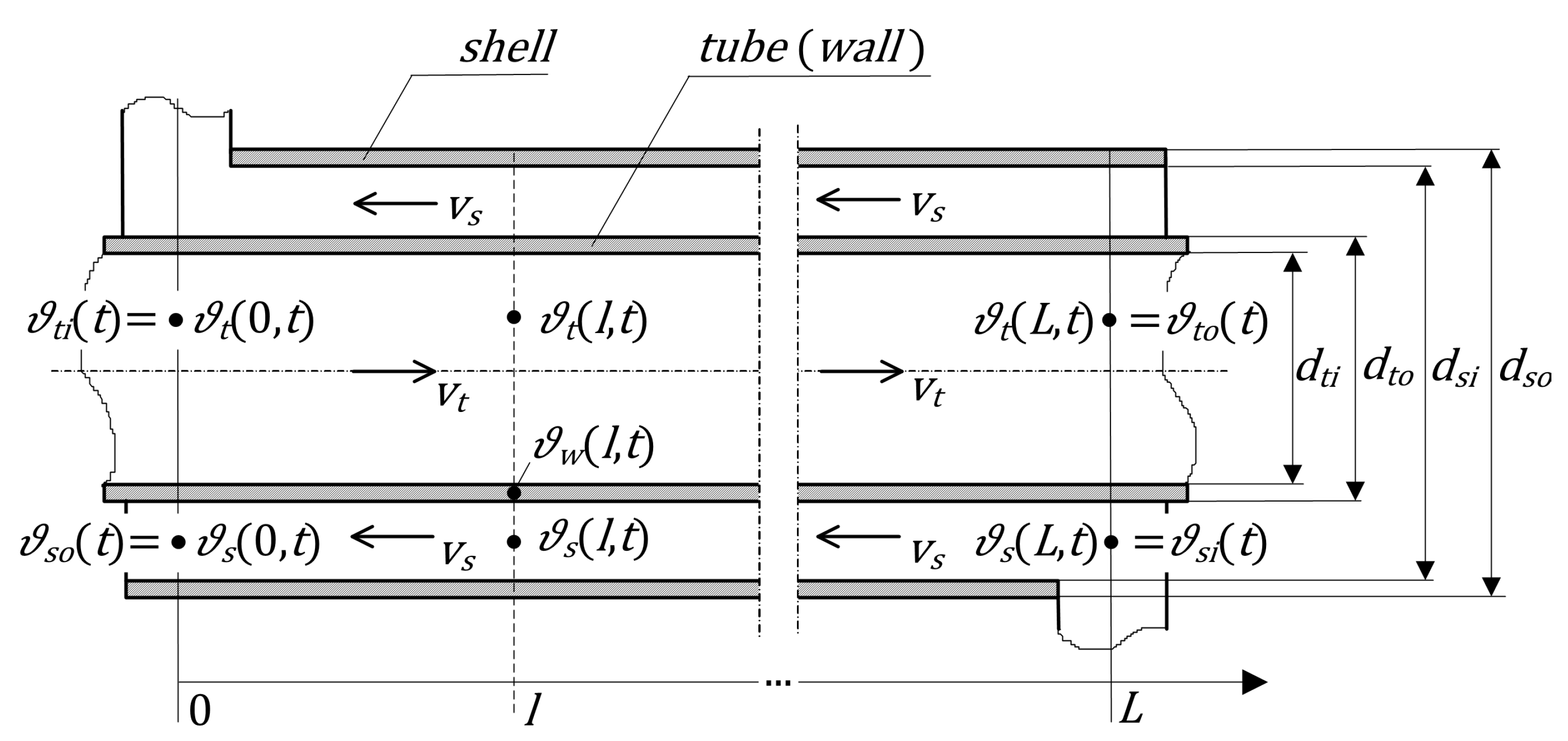
15], and here we focus on the second case illustrated in the schematic of
Figure 1. As will be shown later, the counter-flow mode considered here is more efficient and, therefore, used more often.
2.1. Governing PDEs
The mathematical model for the considered heat exchanger, like any real system model, should be based on some trade-off between its simplicity and accuracy. Since we are interested in a model that would be useful from the control theory point of view, we derive it based on some typical assumptions (see Section 2.1. in [
15]). Taking into account those simplifications, the dynamical model of the considered double-pipe heat exchanger is governed by the following system of PDEs [
7,
8,
14,
27,
28,
29]:
with
denoting the time,
—the space variable,
,
,
,
—the constant parameters depending on the dimensions and the physical parameters of the exchanger:
where
d is the diameter,
—the density,
c—the specific heat,
h—the heat transfer coefficient (subscripts are the same as for the temperatures in
Figure 1).
The
initial conditions which are usually required to obtain a unique solution of the PDEs (
1)–(3) are assumed as follows:
where
are the functions describing the initial temperature profiles.
Equations (
1)–(
5) are to this point consistent with those presented in [
15], where the double-pipe heat exchanger working in the parallel-flow mode was considered. The most important difference which, as will be shown later, has a significant impact on the dynamical properties and, consequently, on the efficiency of the exchanger, concerns the form of the
boundary conditions. Now we are considering the counter-flow configuration with
and
(see
Figure 1), for which these conditions have the following form:
with
and
representing the inlet temperatures of the tube- and the shell-side fluids, which can be therefore seen as the
input signals to the heat exchanger system (see
Figure 2). Their variations in time influence the temperature distribution of both fluids along the exchanger, and, consequently, their outflow temperatures,
which can be seen as the
output signals of the heat exchanger system.
2.2. Spatially Distributed Irrational Transfer Functions
Assuming the boundary input signals given by Equations (
6) as well as the boundary output signals in Equations (
7), the
spatially distributed transfer functions for the considered heat exchanger can be written as the following 2 × 2 matrix
with the elements defined as
for zero initial conditions in Equations (
5). We assume here that the parameter
s in the expression
indicates the Laplace transform of
in the variable
t, i.e.,
.
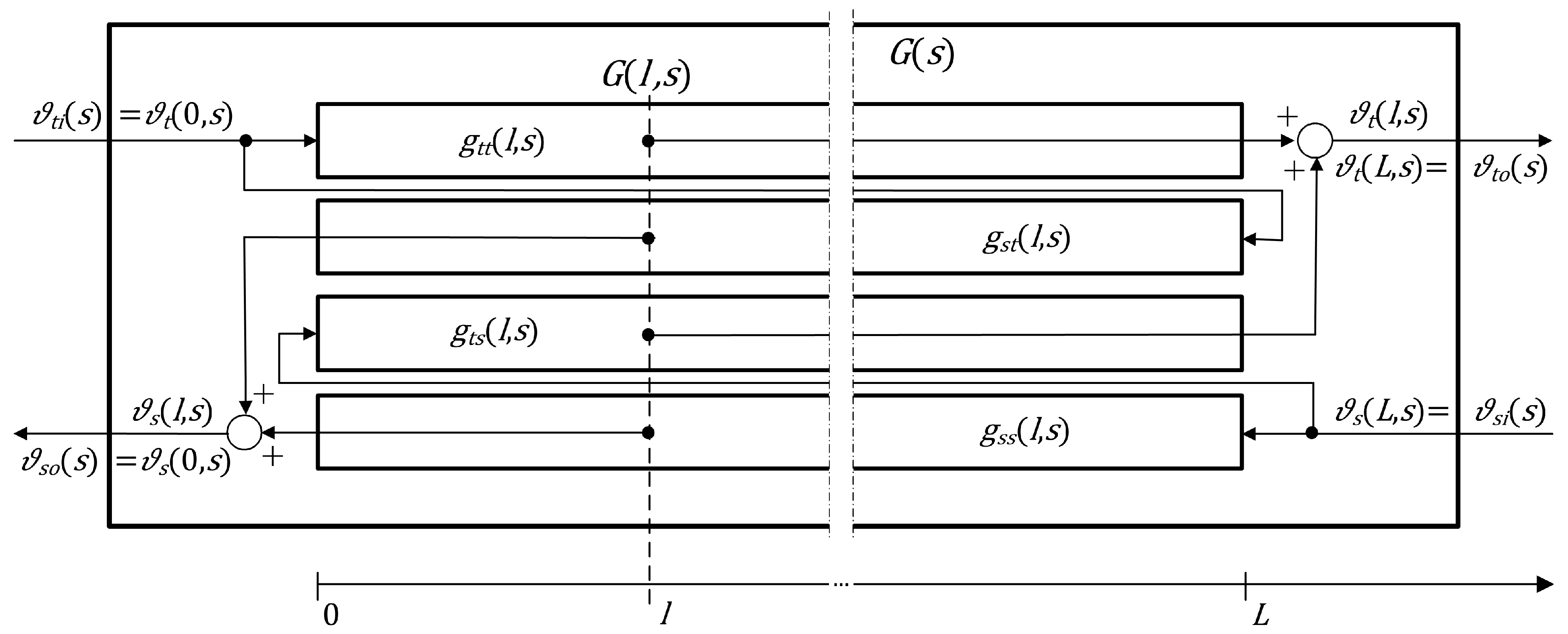
The block diagram for the considered spatially distributed transfer function model is shown in
Figure 2. The temperature distribution of both fluids along the exchanger can be therefore expressed by the following Laplace-domain equations:
where the individual transfer functions defined by Equations (
9) take the following form (for their derivation see Section 3.2 in [
14]):
where
and
As in the case of the parallel-flow configuration considered in [
15], we obtain here irrational expressions containing exponential functions
and
resulting from the convective heat transport, as well as the square root function in Equation (
17) which is typical of heat conduction phenomena. However, due to the different boundary conditions representing the input signals in Equations (
6), the above expressions for the transfer functions are different from those obtained for the parallel-flow configuration—see Equations (12)–(15) in [
15].
Assuming
in
and
, as well as
in
and
, we can obtain the
boundary transfer functions which describe the dependence of the Laplace-transformed outflow temperatures
and
of both fluids on their inlet temperatures,
and
. As in Equation (
8), these transfer functions can be grouped into the following matrix
which will be later referred to as the
boundary transfer function matrix of the exchanger.
Zero heat conduction. Assuming no heat conduction through the wall of the exchanger (i.e.,
in Equations (
4)), we obtain
in Equations (
1)–(3) and
in Equations (
16), and, consequently,
in Equation (
17). For this case the spatially distributed transfer function matrix
in (
8) takes the following simple form:
being the time delays of the tube- and shell-side fluids, respectively, and the boundary transfer function matrix (
18) is given by
The resulting system now consists of two independent pure time-delay subsystems with the time delays and , representing two fluids “traveling” along the exchanger in opposite directions with unchanged inlet temperature profiles, and .
2.3. Frequency Responses
In the expressions for the transfer functions introduced in
Section 2.2,
s is a complex variable which can be written as
where
and
are real numbers and
is the imaginary unit. By setting
to zero, or, equivalently, by making the substitution
where
can be interpreted as the angular frequency, we transform these expressions from the Laplace domain to the Fourier domain. Consequently, such a substitution allows us to evaluate the frequency response of the system which can be then written in the following form:
where
is its modulus representing the system gain
for the sinusoidal input signal with frequency
,
and
is its argument which represents the phase shift between output and input sinusoidal signals,
As can be easily seen, the modulus
and the phase shift
depend here not only on the angular frequency
as in case of LPS, but also on the space variable
l. Therefore, the plots of the frequency responses can be presented here in the 3D form. Another option is to show these responses as classical 2D plots evaluated for a fixed value of the space variable
l, e.g., for the system outputs representing in our case the exchanger outflow points—see Equations (
7). Two types of such frequency response graphs are commonly used in control theory applications: Nyquist and Bode plots, and some examples of them obtained for the considered counter-flow heat exchanger will be shown later in
Section 4.
2.4. Steady-State Responses
The steady-state temperature profiles can be calculated by assuming the time derivatives in Equations (
1)–(3) equal to zero, and solving the resulting boundary value problem with the boundary conditions (
6) given by the constant inlet temperatures of both fluids,
and
(see [
14,
15]).
Another alternative way of determining the steady-state responses consists of considering them as a special case of the system frequency responses evaluated at
. Consequently, they can be obtained by setting
in the transfer functions expressions (
12)–(
17). Based on this idea, the steady-state temperature profiles
and
can be determined from Equations (
10) and (
11) by assuming
and constant inlet temperatures
and
. As a result we obtain the following expressions:
with
being the steady-state spatially distributed transfer functions (
12)–(
15), with
,
,
,
and
given by (
16) and (
17).
The steady-state outflow temperatures of both fluids can be easily determined by inserting
in Equation (
25) and
in Equation (
26). Finally, the steady-state temperature profile of the wall can be then calculated from Equation (2) as
Some examples of the steady-state temperature profiles inside the double-pipe counter-flow heat exchanger will be shown later in
Section 4.
3. Approximate Model of the Heat Exchanger
In the current section we deal with the finite-dimensional approximation of the infinite-dimensional model of the double-pipe counter-flow heat exchanger introduced in
Section 2. For this purpose, we use the semi-analytical method of lines in order to reduce PDEs (
1)–(3) to a set of ODEs. Consequently, the irrational transfer functions
presented in
Section 2.2 are replaced here by their rational approximations
. Using the rational transfer function model, the approximate frequency responses and the approximate steady-state temperature profiles can easily be derived, as shown in
Section 2.3 and
Section 2.4, and compared with the “original” ones, i.e., with those resulting from
.
3.1. MOL Approximation
The principle of the method of lines (MOL) is to replace the spatial derivatives in a PDE by their finite difference approximations. As a consequence, only the time derivatives remain in the resulting expressions which then become ODEs [
15,
30,
31,
32]. In order to obtain the MOL-based approximation model of the double-pipe heat exchanger under consideration, we here use the finite difference method. For the considered counter-flow mode with
and
, we will use the
backward difference approximation for Equation (
1) and the
forward difference method for Equation (3). This means that we will replace the spatial derivatives with their algebraic approximations (see [
33]):
where
are the tube- and shell-side temperatures, respectively, evaluated at the spatial discretization nodes
,
. Moreover, we assume here that
and
represent the boundary nodes, and
are the spatial grid sizes. In general,
can have different values for different
n, which means that the nodes can be unevenly distributed over the spatial range
.
As a result, we obtain the approximation model in the form of a system of 3
N ODEs. Single
nth spatial section of the exchanger is described here by the following three state equations:
for
, where
in (
32) and
in (33) represent the boundary inputs in (
6):
The initial conditions (
5) take here the following discrete form:
representing the initial temperatures defined for
N spatial nodes,
,
,
…,
.
Therefore, each nth spatial section of the considered ODE model can be seen as a third-order dynamical subsystem with the following properties:
A three-element vector
of the
nth section state variables,
representing the tube-side, wall and shell-side temperatures, respectively, evaluated at
;
A two-element vector
of the
nth section output signals,
made of first and third components of the section state vector (
37), where
and
can be seen as the approximations of the boundary outputs (
7) representing outflow temperatures,
A two-element vector
of the
nth section input signals, which for
are given by the output signals of the adjacent sections,
and for
and
also by the boundary conditions (
6) representing the inflow temperatures,
The state Equations (
32)–(34) together with their initial conditions (
36) can be seen as an approximate representation of the heat exchanger dynamics. Therefore, the state and output equations for the single
nth section can be compactly written, using the state (
37), output (
38) and input (
40)–(
42) vectors in the following linear state-space form,
with
being the state, input and output matrices for the
nth section, respectively.
Comparing the section matrices in Equations (
45) and (
46) with those obtained for the parallel-flow configuration (see Equation (41) in [
15]), we can state that the only differences are: the additional minus sign in front of
(which itself is negative) and
instead of
in the denominator below
in
and
. Therefore, assuming uniform grid size (i.e.,
for
), we obtain the same state-space representation of the single section as for the parallel-flow mode. Consequently, the considerations regarding the stability of the single section as a dynamical subsystem remain also the same. Since all physical parameters in Equations (
1)–(
4) as well as
and
in Equations (
31) are positive, the state matrix
in (
45) is diagonally dominant with negative diagonal elements which ensure the stability of the single section [
15].
The main difference between the approximation models for the parallel- and the counter-flow configurations is in the way the sections are interconnected with each other. As will be shown later, such different interconnections result in a quite different systems, with distinct dynamical as well as steady-state properties.
3.2. Approximate Rational Transfer Functions
3.2.1. Single Section
Assuming that the transfer functions for the single section are given by the following 2 × 2 matrix
with
and zero initial conditions, we can obtain the transfer function matrix
in (
47) from the following well-known transformation [
27],
which results in the following rational expressions for the transfer functions in (
48):
with the coefficients of the numerator (
b) and the denominator (
a) depending on the system parameters in Equations (
1)–(
4) and the spatial grid sizes
and
in (
31).
Assuming a uniform spatial grid with
for
, the transfer functions given by Equations (
50) are the same as those obtained for the parallel-flow mode. As can be easily seen, the denominator polynomial is common for all transfer functions in (
50) and represents the characteristic equation of the section state matrix
in (
45). Therefore, the stability analysis performed in
Section 3.1 in terms of eigenvalues of
remains valid for the poles of
[
15].
3.2.2. N-Section Approximation Model
The approximation model for the parallel-flow heat exchanger was obtained in [
15] by the cascade interconnection of
N individual sections, each described by the transfer function matrix
,
. This interconnection schema resulted in the approximate distributed transfer function expressed simply as the matrix product of the transfer functions of individual sections,
for any
where
, and
for the special case of the approximate boundary transfer function matrix.
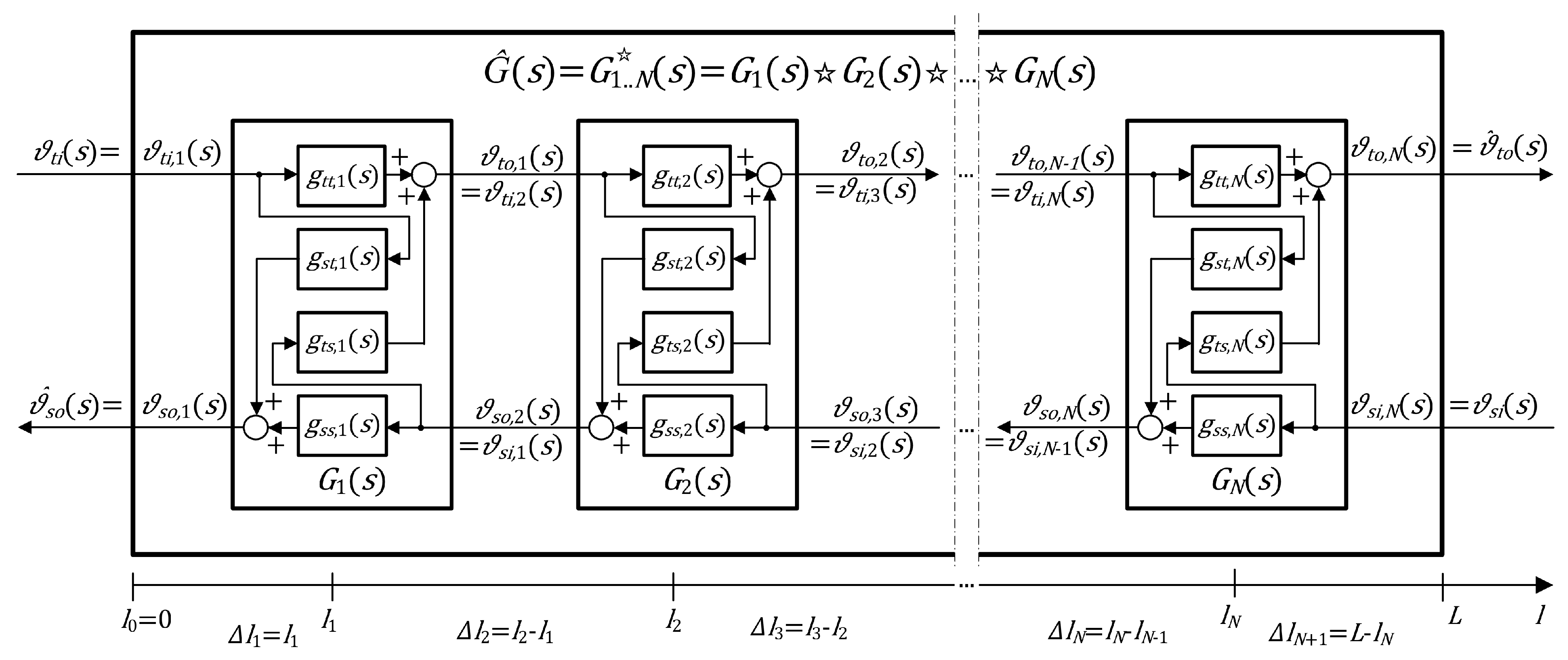
However, for the considered counter-flow configuration, the individual sections of the approximation model are interconnected in a different way, as shown in
Figure 3 (compare to Figure 4 in [
15]). Therefore, it would be advisable to find a certain matrix operator analogous to the classical matrix product in Equations (
51) and (
52), which would correspond to the connection structure presented in
Figure 3.
After an extensive literature review, we found that the appropriate mathematical representation of the considered approximation model can be obtained using a general concept of linear fractional transformation (LFT) which plays an important role in control theory [
17]. More precisely, it can be shown that the interconnections of
Figure 3 can be expressed using the Redheffer star product (RSP) which is also used, e.g., in quantum mechanics and quantum field theory [
20,
21], as well as in the scattering of acoustic and electromagnetic waves in media [
22,
23,
24].
RSP of two transfer function matrices. We consider two
transfer function matrices,
whose elements can be scalar transfer functions or transfer function matrices of appropriate dimensions. The RSP of these two matrices is given by the following
matrix (see [
17,
19,
23]):
where
and
I is the identity matrix of appropriate dimension.
Based on the above definition, it can be shown that the approximate boundary transfer function matrix
which is defined as follows:
with
for zero initial conditions, can be calculated as the following RSP:
where
are the transfer function matrices of individual spatial sections given by Equations (
47)–(
50). It is also possible to use RSP for calculating the approximation
of the spatially distributed transfer function matrix
introduced in
Section 2.2. However, the appropriate expressions are more complicated here than for the case of the boundary transfer function matrix and are omitted here for the sake of space.
Another question which needs to be addressed here is the stability of the resulting dynamical system of
Figure 3. As shown in [
15], for the parallel-flow mode we obtained the approximation model in the form of a cascaded structure, which is stable if all its sections represent stable dynamical subsystems. In the present case, we are additionally dealing with some internal positive feedbacks which are clearly visible in the diagram of
Figure 3 as well as as the term
in Equations (
55) and (56), and as
in Equations (57) and (58). Therefore, an additional condition must be met in order to ensure the stability of this feedback-based structure, and this condition can be expressed, e.g., by the small gain theorem [
34,
35]. According to this theorem, the product of the gains of the subsystems forming the feedback loop should be strictly less than one over all frequencies, and this condition is usually met in our case. Moreover, as shown in Chapter 3 of [
36], different interconnections of stable passive dynamical systems again result in a stable passive system. This result remains valid also for the special case when these interconnections are given by the RSP (see Proposition 17 in [
37]).
The frequency and the steady-state responses for the considered approximation model can be obtained in a similar manner to that presented in
Section 2.3 and
Section 2.4, respectively. Having determined the rational transfer function matrix
, the approximate modulus
and argument
can be calculated using Equations (
23) and (
24), respectively. On the other hand, the approximate steady-state temperature profiles
,
and
can be calculated based on
, similarly as in Equations (
25)–(
28).
4. Results and Discussion
In order to demonstrate the results of the discussed approximation method, we consider here a double-pipe heat exchanger with the following parameter values in Equation (
4):
= 1000
(water),
= 7800
(steel),
=
= 4200
(water),
= 500
(steel),
=
= 6000
,
= 0.09 m,
= 0.1 m,
= 0.15 m,
L = 5 m, which result in the following generalized parameters of the PDEs (
1)–(3):
We also assume the following values for the tube-side and the shell-side fluid velocities:
1 m/s,
= −0.2 m/s, where the negative value of
indicates the counter-flow mode (see
Figure 1).
Consequently, the infinite-dimensional representation of the considered heat exchanger with the boundary inputs (
6) is given by the irrational transfer functions (
12)–(
15), where the parameters
,
,
and
in (
16) and
in (
17) are evaluated using the numerical values of
,
,
and
in (
62). These irrational transfer functions will be considered as a reference for the approximate rational transfer functions of different orders, i.e., transfer functions evaluated for different numbers
N of spatial sections.
Assuming, for example, that the spatial domain
is divided into
uniform spatial sections, we obtain the following grid size:
and, consequently, the following matrices of the state-space model in (
45) and (
46):
with the negative real eigenvalues of
:
which mean that the single section can be seen as an exponentially stable dynamical subsystem.
The transformation (
49) results in the following elements of the section transfer functions matrix
:
with the poles equal to the eigenvalues in Equation (
65).
Up to this point, the construction of the approximation model is almost identical to the parallel-flow heat exchanger considered in [
15]. In particular, assuming the same physical parameters of the exchanger, we obtain the same state-space and transfer function matrices for the single section of the approximation model.
The main difference between the approximation models for the parallel- and the counter-flow regimes consists in how the sections are interconnected to each other. As we recalled in
Section 3.2.2, for the parallel-flow operation the cascade interconnection was applied resulting in the approximation model given by the ”usual“ matrix product of the section transfer function matrices—see Equations (
51) and (
52). For the considered counter-flow configuration we need to apply the RSP of the section transfer function matrices, which is given by Equations (
61) and (
53)–(58). It can be easily shown that the gains
for all the transfer functions in (
66) are strictly less than one over all frequencies, which results in the stability of their feedback interconnections, and which, consequently, ensures the stability of the resulting approximation model. Such different interconnection of the sections entails quite different dynamical properties of the resulting model, as compared to the previously analyzed one. This difference will be reflected, among others, in their different frequencies and steady-state responses.
4.1. Frequency Responses
Some examples of the three-dimensional frequency response plots for the so-called hyperbolic systems of balance laws, showing their dependence on both the angular frequency
and the single space variable
l, were presented in our work [
14]. However, as mentioned in
Section 2.3, taking into account the control task we are usually interested in the classical 2D Nyquist and/or Bode plots evaluated at the system outputs, which in our case of the counter-flow heat exchanger are situated at
(outflow temperature
) and at
(outflow temperature
). Therefore, below we compare such classical frequency plots resulting from the irrational transfer functions
introduced in
Section 2.2, and from their rational approximations
analyzed in
Section 3.2.
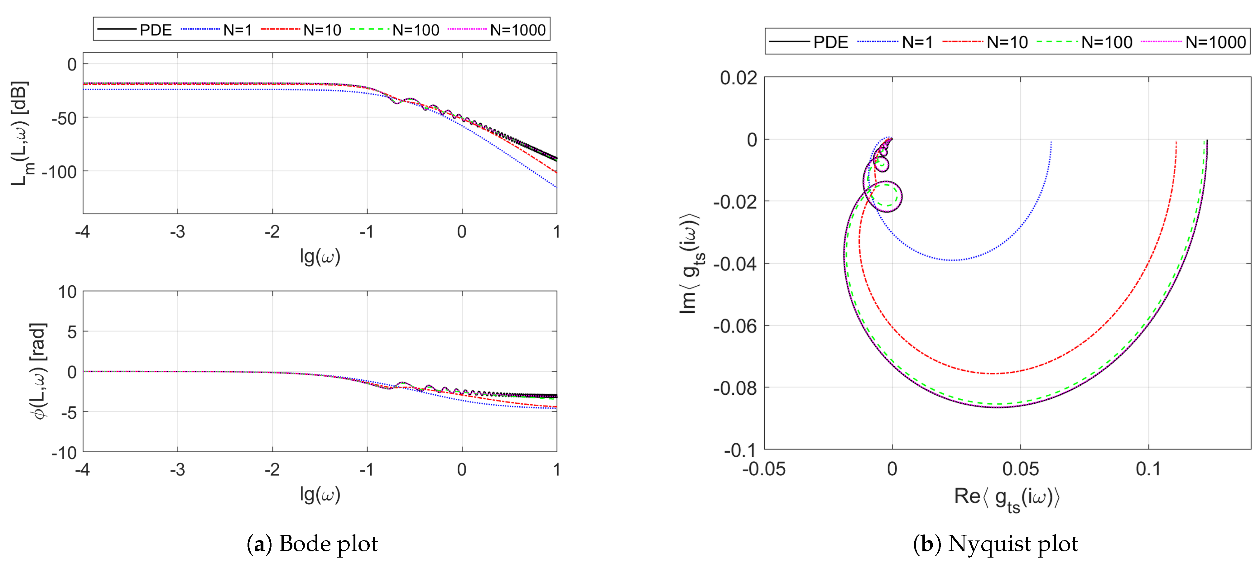
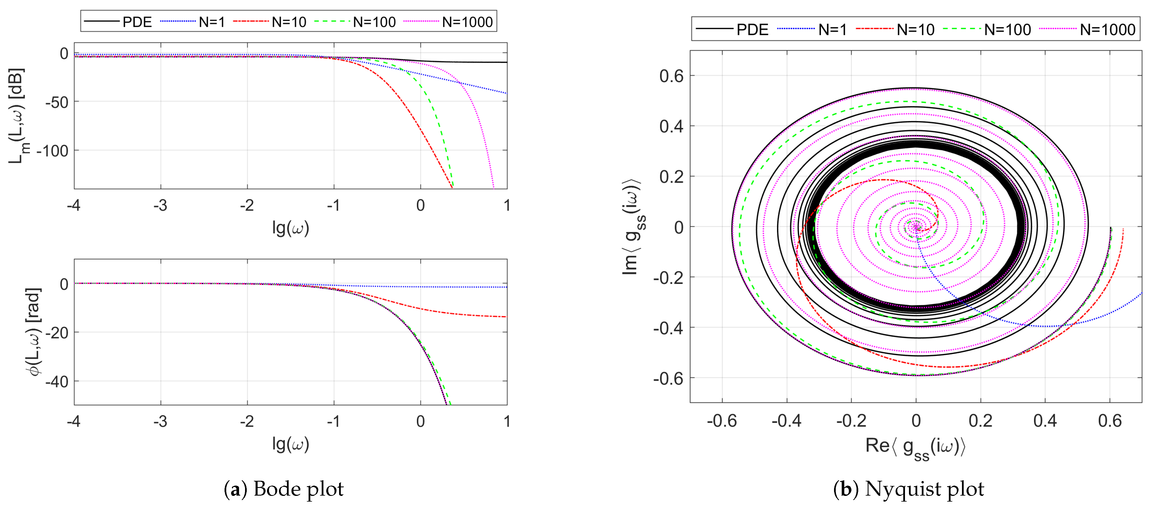
Figure 4 presents the Bode (
Figure 4a) and Nyquist (
Figure 4b) plots of the frequency responses resulting from the boundary transfer function
of the considered double-pipe heat exchanger working in the counter-flow regime. We can see on these plots both the reference frequency response
resulting from the irrational transfer function
given by Equation (
13) for
, as well as the frequency responses obtained from its rational approximations
for different numbers
N of uniform spatial sections. As in the case of the parallel-flow exchanger considered in [
15], we can also notice here some oscillations in the Bode diagram of
Figure 4a, which can be observed as the “loops” on the Nyquist plot of
Figure 4b. These oscillations are due to the resonance-like phenomena taking place inside the exchanger, which are confirmed both by the mathematical models as well as by the laboratory experiments (see [
38]).
When it comes to the differences between the frequency responses
for the parallel- and counter-flow modes, one can see that the phase shift is significantly smaller here than it was for the parallel-flow mode—see Figure 5a,b in [
15]. The phase shift does not exceed
rad for
here, which can be observed both on the phase diagram of the Bode plot, as well as in the Nyquist plot which lies completely in the fourth and third quadrants of the complex plane and does not enter the second and first quadrants, as was in the parallel-flow mode. As is commonly known, a large phase shift and the associated time delay between the input (control) and the output (controlled) signals has a negative effect on the feedback control. Therefore, it can be stated that, from the control theory viewpoint, the counter-flow configuration is more preferable than the parallel-flow one. Another even more significant advantage of this configuration comes from the more favorable steady-state operating conditions (i.e., temperature profiles), which will be analyzed later in
Section 4.2.
Moving on to the approximation quality, it should be clear from the results of
Figure 4 that the larger the number of spatial sections, and, consequently, the order of the approximation model, the better the mapping of the original frequency responses.
Moreover, in order to correctly reflect the above-mentioned oscillations, a relatively high-order rational model is needed which is able to approximate these high-frequency peculiarities [
15].
Figure 5 shows the frequency responses obtained for the transfer function channel
of the counter-flow heat exchanger. As easily seen, the dominating time-delay nature of this channel which is related to the convective heat transport results in the original frequency response having no limit at infinity. As a consequence, the approximation task is even more difficult here than in the previous case. The approximation models
of increasing order try to mimic the reference frequency response, but the rational approximation is possible here only over a certain finite frequency band—see results of [
39].
Due to the symmetry of the system, the frequency responses of the two other boundary transfer function channels, and , which are not shown here, are similar to the ones obtained for and , respectively.
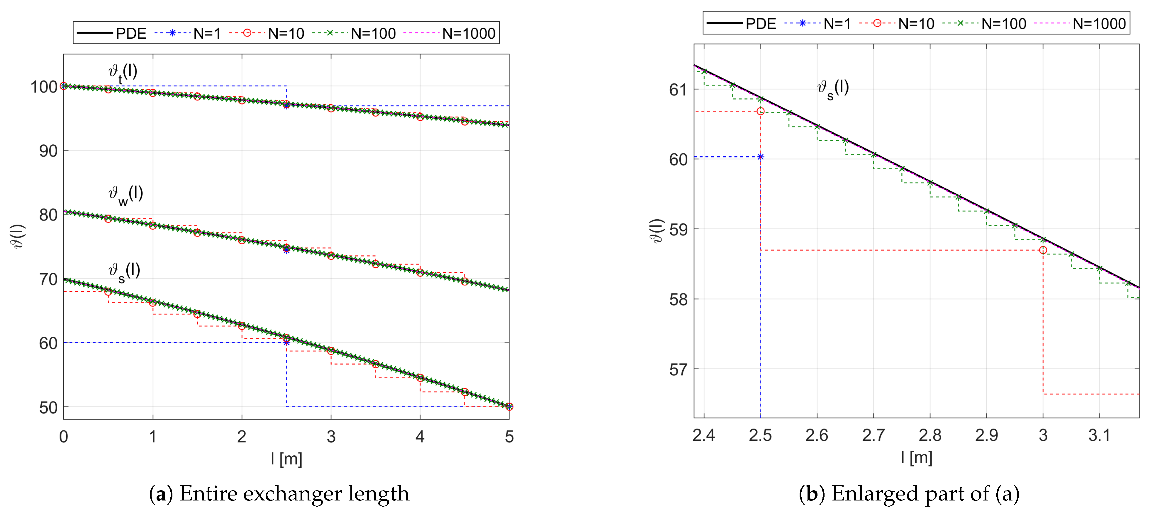
4.2. Steady-State Temperature Profiles
The steady-state temperature distribution of both fluids and the wall of the exchanger were calculated from the spatially distributed steady-state transfer function model
given by Equations (
25)–(
28), as well as from its approximations
of different orders discussed in
Section 3.2.2. The temperature profiles obtained for the following constant inlet fluid temperatures:
,
are shown in
Figure 6.
As confirmed by the presented results, the steady-state temperature distribution of the fluids and the wall is more favorable for the counter-flow configuration considered here than for the parallel-flow one (see Figure 7 in [
14]). The outlet temperature
of the heated fluid is closer here to the inlet temperature
of the heating fluid, and the more uniform difference between
and
contributes to the more uniform heat transfer rate. In addition, the greater uniform temperature difference between the two heat exchanging media reduces the effects of thermal stresses in the material of the exchanger (see [
14,
15]).
When it comes to the results obtained from the approximate transfer function models, it can be seen on the temperature plot of
Figure 6a that the larger the number
N of spatial sections, the more overlap the original steady-state profiles
,
and
by their approximations
,
and
, respectively. For details of the steady-state approximation results, the enlarged part of the
Figure 6a is shown in
Figure 6b.
5. Conclusions
Continuing the research whose outcome is presented in our paper [
15], in the current work we have shown some new results concerning the approximate rational transfer function model for the double-pipe heat exchanger, now operating in the
counter-flow configuration. This model can be used, e.g., in the control system design procedure using the conventional, relatively simple control algorithms provided for LPSs, without recourse to sophisticated, infinite-dimensional control approaches dedicated for DPSs.
As confirmed by simulation, the considered counter-flow configuration is better than the parallel-flow one. This is mainly due to the more preferable steady-state temperature conditions, although the better dynamic properties expressed by a smaller phase shift between the input and output signals are also important from the control theory viewpoint. We have also shown that subsystems with different approximation properties depending on the dominant physical phenomena can coexist within the same dynamical system.
To mention the disadvantages of the presented approach, it should be noted that the obtained approximation model can be of very high order—especially for the transfer function channels and dominated by transport delays. Therefore, it would be recommended in the next step to perform some model reduction methods in order to obtain lower-order models.


