Modeling of Small Productive Processes for the Operation of a Microgrid

Abstract

Small productive processes (SPPs) are promising drivers that promote the economic use of energy in microgrids (MGs). Both the complex nature of the SPPs and voltage variations make the operation of MGs challenging, since the quality of an energy management system’s (EMS) decisions depend on its characterization. The aim of this work is to propose a methodology for SPPs modeling, and to consider the influence of voltage on load consumption, which has general validity, and can be efficiently integrated into different MG EMS approaches. For this purpose, a novel extended multi-zone ZIP approach for the characterization of SPP loads and sensitivity to voltage changes is proposed. The associated framework herein presented was assessed using actual data collected from SPPs installed near the city of Arica, in northern Chile. The results showed that the proposed methodology was capable of representing the complex load behavior of the SPPs, properly considering the voltage influence. These results were compared with those obtained through common approaches found in the literature. The effectiveness of the proposed approach in representing SPP loads and their sensitivity to voltage changes was verified. The proposed scheme can be efficiently integrated into a wide range of EMS for MGs that include SPPs.

1. Introduction

Microgrids (MGs) are well-known for “taking advantage” of local renewable energy sources (RES) in order to provide energy to communities and, thus, ensuring sustainable development [1,2]. Therefore, the microgrid industry is expected to grow in future years [3].

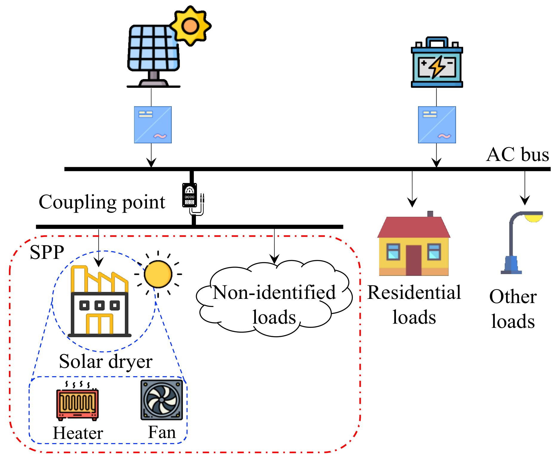
Alternatively, productive use of energy (PUE), primarily in rural settlements, has received much attention in recent years due to its potential to contribute to the economic growth and social progress of communities [4]. Consequently, the benefits of MGs combined with the PUE have stimulated the deployment of several small productive processes (SPPs), which can be embedded in MGs (see Figure 1) and offer different economic benefits to communities.

According to the Deutsche Gesellschaft für Internationale Zusammenarbeit (GIZ), the PUE is defined as “agricultural, commercial, and industrial activities involving electricity services as a direct input to the production of goods or provision of services” [5]. In this context, SPPs consist of integrating technological solutions in traditional and small-scale productive activities to add value to their goods and services. These SPPs may include small-scale industrial and household loads, distributed energy resources (DERs), e.g., photovoltaic panels (PV), and in some cases, a storage unit (see Figure 1).

Generally speaking, SPPs may include an array or a mix of different electric devices (e.g., cooling and heating devices, motors, drills, conveyor belts, chainsaws, dryers, etc.) [6]. These as a whole transform the inputs into goods or services providing economic benefits to communities by adding value to their traditional productive activities.

Due to the benefits of the SPPs mentioned above, several successful initiatives have been implemented worldwide, especially in rural communities. Some small processes are, for example, milling processes of maize (corn) to produce flour to sell in the local community and water treatment systems for bottled water [4]. Moreover, more general productive processes have been implemented, such as heating and cooling systems, grain mills, crop farming, food processing, milking systems, and incubators for poultry farming, among others [7]. More examples regarding the implementation of SPPs in several countries can be found in [8].

In Chile, through the Ayllu Solar initiative, some SPPs have been implemented to foster the sustainable development of the rural communities in the Arica and Parinacota region located in northern Chile [9]. The Ayllu Solar project consists of four main representative projects that make intensive use of solar energy, such as an alpaca fiber processing center [10], farming of river shrimp, a center for processing agricultural products, and the upgrading of tourism in pre-Hispanic routes through PV technology [9].

On the other hand, MGs are small distribution systems, which consist of local generation systems (e.g., PV, wind turbines, fuel cells, etc.), energy storage systems (e.g., batteries, flywheels, etc.), loads, either conventional or flexible [11], and more recently, the SPPs [9].

For adequate and efficient operation of MGs, different approaches of energy management systems (EMSs) are used [12]. Roughly speaking, an EMS is in charge of matching the generation and demand by determining:

• The amount of energy provided by programmable local generators (such as diesel generators).
• The amount of energy provided to/taken from the grid by the energy storage systems (ESSs).
• The amount of flexible demand that must be fed.

These decisions are made based on both the expected electric energy demand (flexible plus conventional/non-flexible) and the available power from local DERs based on variable generation technologies, such as solar [12]. On the other hand, due to the small size of MGs, the load variability rises, and the aggregation or smoothing effect is considerably reduced in contrast to that of large power systems [11]. Moreover, considerable voltage variations in MGs may occur more frequently in isolated ones. These variations will influence the EMS operation strategies.

SPPs have a particular “behavior” involving the interaction between several types of loads (not only conventional ones, but also complex ones). Thus, the uncertainty increases, which can directly impact the reliable, secure, and economic operation of such MGs.

As stated above, load modeling and, consequently, expected load consumption play a key role in the operation of MGs. Since, based on its characterization, the expected electric energy demand is estimated and, therefore, the decisions of the EMS are made [13,14,15].

However, the pattern of use of the SPP loads and the timing at which they are employed change from one process to another based on complex dynamics and weather conditions. Moreover, SPPs generally include loads that are sensitive to voltage variations [16]. These voltage variations under normal MG operating conditions (i.e., 1 p.u. ± 5%) [17,18] may increase/decrease the load consumption of the SPPs. For example, a 5% reduction in operating voltage will decrease the power demand in residential loads by around 7.6% [19]. Thus, this can influence the proper operation and energy management in the MG.

To summarize, the diverse nature of the SPP loads combined with weather-sensible features, make the modeling of such loads a difficult task and a big challenge. Therefore, representing such SPP complex load interactions through a load model, estimating the parameters of such load model, and considering the voltage influence, is still an open research question [16].

One way to represent arrays of loads, with an aggregated approach, is by using the information available at the measurement points. For this purpose, the specialized literature presents different modeling approaches, such as those based on artificial intelligence (AI), e.g., fuzzy models [20] and artificial neural networks (ANN) [21], those based on statistical models, e.g., auto-regressive moving average models (ARMA) [22], and those based on gray box models and black box models [23]. However, such approaches do not directly consider changes in load consumption due to voltage variations, which may affect the MG operation.

Two of the most used models that address this drawback are the ZIP load model [24] and the exponential model [25]. The former has the advantage of representing the entire load behavior through all three load characteristics. In fact, the abbreviation “ZIP” refers to the representation of a load by its constant impedance “Z”, constant current “I”, and constant power “P” characteristics. However, complex loads have a wide nature and complicated behavior. Thus, to represent such complex behavior, some studies have proposed multi-stage or multi-step load models [26,27,28,29]. These models may combine several models at the same time, such as dynamic models, exponential models, ZIP models, etc.

The authors’ first attempt at looking for modeling the SPPs, in the context of MGs, was in the work presented in [30], where the time-variant ZIP load model was used. Nonetheless, the works described above either assume certain known parameters or have only focused on load modeling in specific contexts, and have not considered an integrated approach contemplating MG operation and voltage influence.

To the best of our knowledge, no previous studies have provided a comprehensive methodology to represent the behavior of SPPs in the context of EMS for MG operation. Therefore, to fill this research gap, this paper proposes a methodology for modeling the SPPs for MG operation through an extended multi-zone ZIP model, which is able to:

• Consider the influence and behavior of voltage on load consumption for a new type of complex load called SPPs, which will play a key role in the development of MGs.
• Both represent unnoticeable devices and can manage transitions between zones. This is because the extended multi-zone ZIP model considers a flexible component.
• Identify the contributions of each load category against total load consumption considering the different time zones of the analysis window. This has to do with the structure of the extended multi-zone ZIP model.

More concretely, the proposed methodology ensures that SPP models have general validity and can efficiently integrate into a range of EMS approaches. Nevertheless, thorough detail of EMS operation is not part of the scope of this study. Finally, to assess the proposed methodology and its contribution, an application using actual data gathered from productive processes installed in Chile was developed.

The remainder of the paper is organized as follows: Section 2 presents the proposed methodology for modeling of the SPSs for the operation of MG; Section 3 describes the case study; Section 4 presents the results and the discussion; and Section 5 presents the conclusions and future work.

2. Proposed Methodology

As previously mentioned, the SPPs may include complex loads that are sensitive to voltage variations. Hence, the proposed methodology considers such voltage influence to develop the SPP load model.

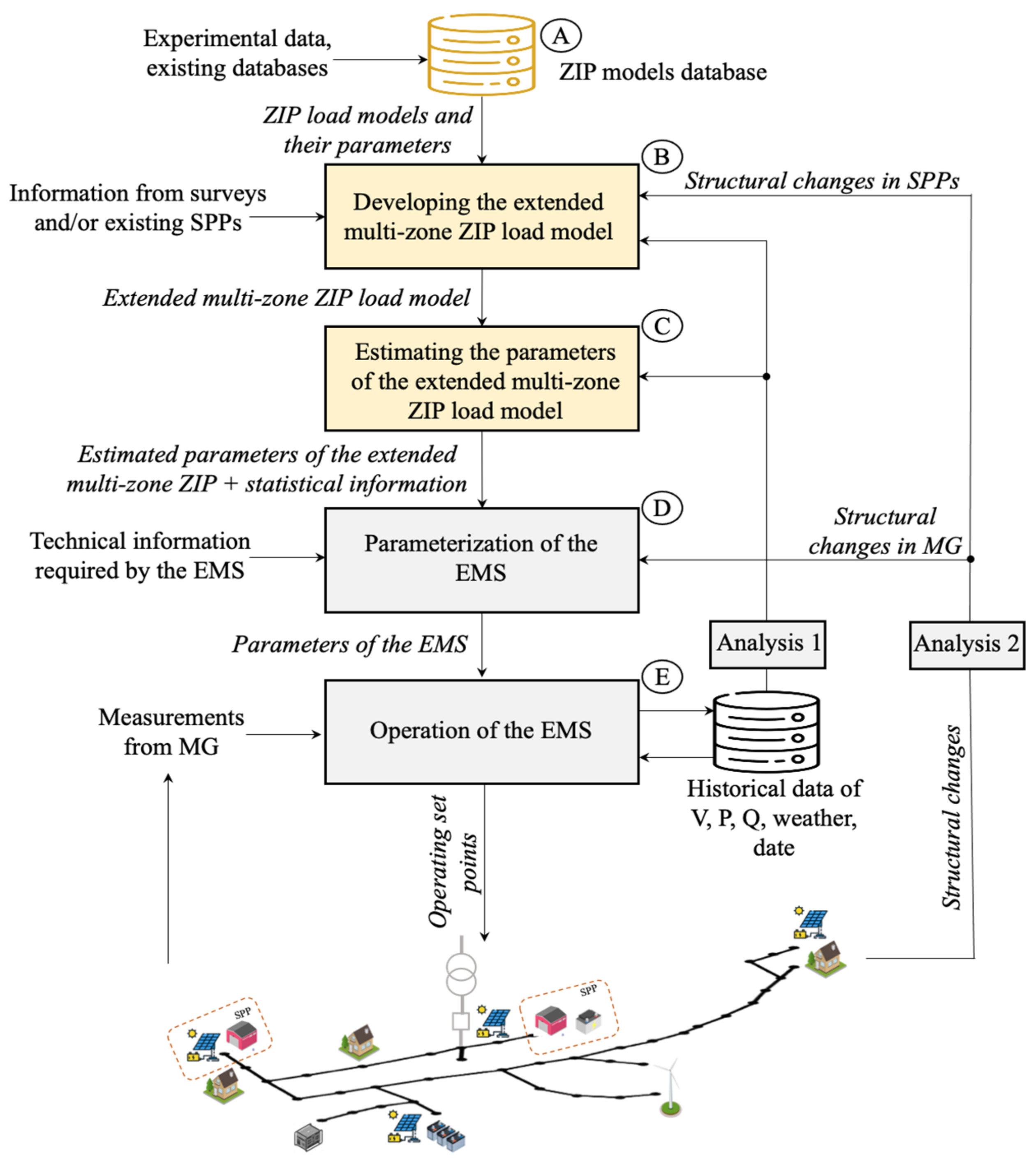
The proposed methodology for modeling the SPPs consists of five main stages with their respective inputs and outputs, as can be seen in Figure 2. In stage A, a database is developed. This database contains the ZIP load models and their parameters for specific devices that an SPP may include. Such ZIP parameters can be obtained from either experimental data or existing databases.

In stage B, an extended ZIP load model is developed. For this purpose, the information gathered through surveys and/or from existing SPPs is considered. This is feasible and convenient, considering the engagement of customers promoted by an MG owner. Then, through the collected information, it is feasible to know the structure of the SPPs and the specific time in which the devices are used (i.e., patterns of energy consumption). Then, the extended ZIP load model combines a generic flexible ZIP, and ZIP load models for specific devices stored in the database created previously. Furthermore, using the patterns of energy consumption, a zone division procedure is performed. Then, an extended ZIP load model is developed for each zone. Consequently, the extended multi-zone ZIP load model can be established.

In stage C, the parameters of the extended multi-zone ZIP load model are estimated. This procedure is performed through an optimization problem and the use of the historical data of power and voltage. In this stage, the estimated parameters of the extended multi-zone ZIP load model and statistical information of residuals are provided. For SPPs in the design phase, it is feasible to use measurements from similar existing SPPs or results from system simulations.

Stage D refers to the parameterization of the EMS. For this purpose, the estimated parameters of the extended multi-zone ZIP load model with the parameters of other loads and DERs are integrated into the system operation modeling of the EMS. Therefore, both, time and spatial correlations are integrated in the overall load forecasting. Moreover, due to the voltage sensitivity of the developed models, an AC approach is recommended. For example, an AC multi-period optimal power flow (OPF) will be able to define the operating conditions for the scheduling horizon of the EMS.

Furthermore, the statistical information (i.e., residuals distribution) produced in stage C, can be used to define the input parameters for stochastic or robust EMS approaches. More concretely, if an abnormal operation occurs, this phenomenon should be captured as part of the stochastic description of the loads (time correlations). Thus, this information should be used by the EMS to assign the necessary reserves to the system. For example, a load surge scenario resulting from simultaneous powering on of a large number of SPPs can be captured through the calculation of a dynamic system reserve margin considered in the MG operation procedure of the EMS.

Additional technical information about MG elements is also integrated at this stage. For example, cost information for generation/storage units, supplementary technical constraints (e.g., maximum and minimum limits, ramps, efficiencies, etc.), and parameters of other individual loads in the MG.

Finally, once the EMS is parameterized, it is capable of performing MG operation (stage E). To achieve this, the EMS gathers measurements of power, voltage, among others, from MG, in addition to historical data regarding power, voltage, weather, and time. After that, the EMS runs its optimizing routines and sends the operating set points to generation/storage units and other devices. This procedure is carried out in a predefined period (e.g., 5 min, 15 min) until a predetermined condition, such as those described below, is detected.

At the $t_{initial}$ all stages (A–E) are performed following the sequence in Figure 2. However, if considerable changes are detected in analysis blocks 1 or 2 at the time $t_{initial}+∆t$, certain stages are conducted again. For example, analysis block 1 evaluates statistical information from historical data. Therefore, if a significant variation in the errors in either the zone transitions or in the zone length is detected, it is necessary to execute stage B and, consequently, the other stages are executed too. For example, if the analysis window is in hours, it is evaluated whether it is improved by extending or reducing the current zone duration. Besides, if new historical power and voltage data exist, then it is necessary to re-estimate the parameters of the extended multi-zone ZIP model by running stage C. Alternatively, analysis block 2 analyzes the structural changes in either the MG or SPPs or both. For example, if new devices are installed in the SPPs, it will be necessary to run from stage A again. Thus, the extended multi-zone ZIP model will include the ZIP models of the newly added devices. Moreover, if analysis block 2 detects structural changes in the MG (e.g., changes in the topology, adding or removing generation units or loads different from those of the SPPs), then it is necessary to execute stage D to re-parameterize the EMS, and include such structural changes.

Finally, the proposed methodology for modeling the SPPs involves the aforementioned five stages. This strategy is compatible with different EMS architectures and approaches. Nevertheless, stages D and E are highly dependent on the specific EMS architecture. Based on the scope defined for this work, stages A, B, and C are thoroughly described in the next sections. Consequently, a comprehensive description of the potential integration of this proposal for different EMS solutions is offered.

2.1. Development of a Database with ZIP Load Models of Specific Devices

As mentioned in the previous section, the ZIP load model is one of the various appealing alternatives for load modeling. The mathematical expressions of the ZIP load models for the active and reactive power at any discrete time step $k$ ($k\in {\mathbb{Z}}^{+})$ are expressed as follows:

$$P_k=P_0\left({\alpha }_1{\left(\frac{V_k}{V_0}\right)}^2+{\alpha }_2\left(\frac{V_k}{V_0}\right)+{\alpha }_3\right)$$

(1)

$$Q_k=Q_0\left({\beta }_1{\left(\frac{V_k}{V_0}\right)}^2+{\beta }_2\left(\frac{V_k}{V_0}\right)+{\beta }_3\right)$$

(2)

$${\alpha }_1+{\alpha }_2+{\alpha }_3=1$$

(3)

$${\beta }_1+{\beta }_2+{\beta }_3=1$$

(4)

where $P_k$ and $Q_k$ are the total active and reactive power consumed by the load at any time step $k$, respectively; $V_k$ is the current voltage at time step $k$; $P_0$ and $Q_0$ are the active and reactive power at nominal voltage $V_0$; ${\alpha }_1$, ${\alpha }_2$, ${\alpha }_3$, and ${\beta }_1$, ${\beta }_2$, ${\beta }_3$ are the ZIP coefficients for the active and reactive power, respectively, and they define the contribution of each feature of the load and must satisfy (3) and (4).

As mentioned earlier, based on information gathered through surveys or information about existing SPPs, it is feasible to know the structure of such SPPs in terms of the type and number of specific devices that they comprise, such as a “fingerprint” of each SPP. Thus, it is possible to acquire the ZIP parameters (i.e., $V_0$, ${\alpha }_1$, ${\alpha }_2$, ${\alpha }_3$, ${\beta }_1$, ${\beta }_2$, ${\beta }_3$) for each potential device used by the SPPs from either experimental data or existing load model databases, for example, from [25,31]. This database will be the main source of information for the next stages.

To illustrate the use of the database, let us assume that an SPP consists of the following devices: (i) a conveyor belt; (ii) an electrical heater; and (iii) two water pumps. Then, the ZIP parameters for each device are acquired and stored in the database. Hence, the parameters${\alpha }_{1,i}$, ${\alpha }_{2,i}$, ${\alpha }_{3,i}$, ${\beta }_{1,i}$, ${\beta }_{2,i}$,${\beta }_{3,i}$ (i ∈ {heater, belt, two pumps}) are available for the next stages. Note that, to define the parameters $P_0$ and $Q_0$ it is necessary to know the number $m$ ($m\in {\mathbb{Z}}^{+})$ of devices of each type. Consequently, the parameters $P_0{}^{\prime }$ and $Q_0{}^{\prime }$ for each type of device are defined as (5) and (6).

$$P_0{}^{\prime }=m·P_0$$

(5)

$$Q_0{}^{\prime }=m·Q_0$$

(6)

Moreover, this example considers two pumps, thus,

$$P_0{{}^{\prime }}_{pump}=2·P_0{}_{pump}$$

(7)

$$Q_0{{}^{\prime }}_{pump}=2·Q_0{}_{pump}$$

(8)

Besides, for the heater and the belt $m=1$, hence,

$$P_{0,agg}=P_0{{}^{\prime }}_{pump}+P_0{{}^{\prime }}_{heater}+P_0{{}^{\prime }}_{belt}$$

(9)

$$Q_{0,agg}=Q_0{{}^{\prime }}_{pump}+Q_0{{}^{\prime }}_{heater}+Q_0{{}^{\prime }}_{belt}$$

(10)

2.2. Development of the Multi-Zone ZIP Load Model

2.2.1. Extending the ZIP Load Model

Although the ZIP model captures the variations of load based on voltage profile, uncertainties of load behavior in the SPPs could remain. In fact, some devices from the survey/cadaster could be missed or the assigned device from the database could mismatch the load behavior for specific devices. Thus, the first extension of the ZIP model based on the incorporation of a generic extra ZIP component is proposed. More concretely, a time-variant ZIP load model is used to account for these changes [32]. The time-variant ZIP component for the active power is thus mathematically expressed as (12). Moreover, for notation simplicity, (11) is established in the remainder of this paper, hence,

$${\tilde{V}}_k=(V_k/V_0)$$

(11)

$$P_k=P_{0,k}\left({\tilde{\alpha }}_{1,k}{\tilde{V}}_k^2+{\tilde{\alpha }}_{2,k}{\tilde{V}}_k+{\tilde{\alpha }}_{3,k}\right)$$

(12)

where $P_k$ represents the active power at time step $k$, $P_{0,k}$ stands for the nominal active power at nominal voltage $V_0$, $V_k$ is the current voltage at time step $k$, ${\tilde{\alpha }}_{1,k}$, ${\tilde{\alpha }}_{2,k}$, ${\tilde{\alpha }}_{3,k}$ are the time-dependent parameters, which represent the load features of constant impedance, constant current, and constant power, respectively. Moreover, as in the conventional ZIP load model case, the coefficients must fulfill (13) for every time step $k$. As for reactive power, the mathematical expression is similar to (12), with the difference that it has to consider the ZIP coefficients for reactive power.

$${\tilde{\alpha }}_{1k}+{\tilde{\alpha }}_{2,k}+{\tilde{\alpha }}_{3,k}=1$$

(13)

On the other hand, electric consumption may change depending on customer behavior, weather, and time of the year. Consequently, by using the information obtained via the surveys, it is also feasible to establish various periods (zones) in which a set of devices is active. Thus, an extra extension to the model that considers the active devices for different time zones is proposed. The zoning procedure is further described in the next section.

Accordingly, the complete extended ZIP load model combines both the time-variant ZIP load model and the ZIP parameters of the set of active devices for each time zone. Let ${\delta }_{i,k}$ denote the contribution of each load category, to the total load consumption. Then, the extended ZIP load model is expressed in (14)–(17).

$$P_k=P_{0,agg,k}\left({\delta }_{1,k}ZI{P}_{flex,k}+{\displaystyle \sum }_{i=2}^r{\delta }_{i,k}ZI{P}_{i,k}\right)$$

(14)

$${\displaystyle \sum }_{i=1}^r{\delta }_{i,k}=1$$

(15)

$$ZI{P}_{flex,k}=\left({\tilde{\alpha }}_{1,k}{\tilde{V}}_k^2+{\tilde{\alpha }}_{2,k}{\tilde{V}}_k+{\tilde{\alpha }}_{3,k}\right)$$

(16)

$$ZI{P}_{i,k}=\left({\alpha }_{1,i}{\tilde{V}}_k^2+{\alpha }_{2,i}{\tilde{V}}_k+{\alpha }_{3,i}\right)$$

(17)

where, $P_{0,agg,k}$ represents the value of nominal active power at nominal voltage $V_0$, $ZI{P}_{flex,k}$ represents the flexible component of the extended ZIP load model for which it is necessary to identify all its parameters (i.e., ${\tilde{\alpha }}_{1,k}, {\tilde{\alpha }}_{2,k}, {\tilde{\alpha }}_{3,k}$) and its contribution ${\delta }_{1,k}$ to total load. On the other hand, $ZI{P}_{i,k}$ represents each device of the SPP, of which their ZIP coefficients (${\alpha }_{1,i}$, ${\alpha }_{2,i}$, ${\alpha }_{3,i}$) are already known (see Section 2.1). Thus, solely the identification of its contribution ${\delta }_{i,k}$ is needed. Equation (15) reflects the contribution of each device of the SPP through the values of ${\delta }_{i,k}$. Finally, the term $r$ ($r\in {\mathbb{Z}}^{+})$ represents the number of devices that belong to an SPP.

Conversely, without any measurement or additional information from the SPP, the initial estimation of the parameters is as described in (18)–(20).

$$P_{0,agg,k}={\displaystyle \sum }_{i=2}^r{P}_{0i}{}^{\prime }$$

(18)

$${\delta }_{1,k}=0$$

(19)

$${\delta }_{i,k}=P_{0i}{}^{\prime }/P_{0,agg}$$

(20)

As measurements are acquired, the set of parameters, including $\left({\tilde{\alpha }}_{1,k}, {\tilde{\alpha }}_{2,k}, {\tilde{\alpha }}_{3,k}\right)$ is estimated for each time interval k. For example, if the time step k corresponds to 10 min, and the measurements are acquired every 10 s, 60 data sets are available for each time step.

2.2.2. Zoning the Extended ZIP Load Model

Based on the information gathered from surveys, the time in which the different devices considered in (14) are active can be known in advance (see Section 2). Thus, a zone division of the analysis window (e.g., 24 h) can be done so that at every zone of the analysis window, just a set of devices is considered. This is useful for both significantly decreasing the complexity of the parameter identification process (because solely a set of parameters are identified instead of estimating all of them), and for properly representing the sensitivity of SPP loads to voltage.

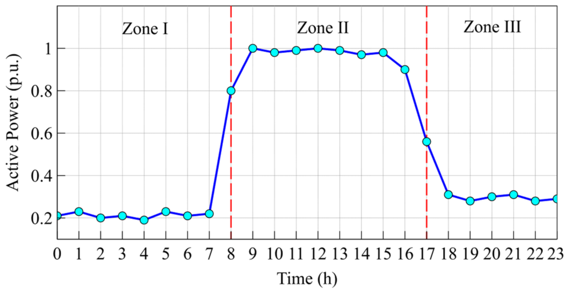
For illustrative purposes, let us consider the active power shown in Figure 3, which was measured at each time step $k$ (every hour). These active power data were collected from a specific location where it is known that (i) lights are active from 5:00 p.m. until 7:00 a.m. of the following day; (ii) industrial activities work from 8:00 a.m. to 5:00 p.m.; and (iii) a water pump and non-identified loads can be active at any time of the day. Hence, based on these patterns of energy use, three zones can be established: zone I (12:00 a.m.–7:59 a.m.), zone II (8:00 a.m.–5:00 p.m.), and zone III (5:01 p.m.–11:59 p.m.).

Table 1. Active devices in each zone.

Zone	Active Devices	Usage Hours	${\mathit{r}}_{\mathit{j}}$
I (j = 1)	lighting + water pump + non-identified loads	12:00 a.m.–07:59 a.m.	3
II (j = 2)	anc. services + water pump + industrial activities + non-identified loads	08:00 a.m.–5:00 p.m.	4
III (j = 3)	lighting + water pump + non-identified loads	5:01 p.m.–11:59 p.m.	3

puts forward the established zones based on the electric demand profile (see Figure 3) and the knowledge regarding the use of energy in the SPP as described above.

It is worth noting that the flexible component of the EMZ-ZIP (i.e., $ZI{P}_{flex,k}$) plays a key role during transitions between time zones. This is because the flexible component is able to represent a combination of devices unnoticeable in the transition. Moreover, the flexible component can be updated at each time step k using the measurements.

Consequently, as the EMZ-ZIP is considerably flexible for both handling the zone transitions and representing unnoticeable devices, the zoning procedure is based on a practical zoning definition, primarily using the information regarding the patterns of energy use collected through surveys. Moreover, the length of the zones can be adjusted according to the procedure described in the analysis block 1 of the proposed methodology (see Section 2).

Finally, based on (14)–(17), and once the zones $j$ ($j\in \left\{1, 2, 3\right\}$) have been established, the general mathematical expression for the extended multi-zone ZIP load model (EMZ-ZIP) is expressed as follows:

$$P_k=P_{0,agg, k}\left({\delta }_{1,k}ZI{P}_{flex,k}+{\displaystyle \sum }_{i=2}^{r_j}{\delta }_{i,k}ZI{P}_{i,k}\right)$$

(21)

where the terms are similar to those of expression (14), with the difference of the term $r_j$ $\left(r\in {\mathbb{Z}}^{+}\right)$ that stands for the number of active devices in each time zone j.

Similarly, the same procedures described for both extending the ZIP model and developing the EMZ-ZIP can be applied for representing the reactive power of the SPPs.

On the other hand, as previously explained, the initial zoning procedure is primarily based on the knowledge regarding the patterns of energy consumption of the SPP (surveys and secondary information). However, the zoning procedure could be improved by considering the measurements of the system after the commissioning period of the SPPs. For this purpose, suitable signals can be the total active power, voltage profile [26], and reactive power. Moreover, for the automated definition of time zones, cluster analysis [33], Markov Chain [34], or artificial neural network techniques [35] can be applied. Nevertheless, the automated definition of the zones is beyond the scope of this manuscript.

2.3. Estimation of Parameters of the EMZ-ZIP Load Model

The parameter identification procedure is performed by using actual measurements and an optimization problem. Let ${\widehat{P}}_k$ be the estimated active power at time step $k$ for zone $j$, and $D$ denote the data set of measurements for each time step k. Then, the set of parameters to be identified is determined by solving the minimization problem in (22).

$$\underset{\begin{array}{c}{P}_{0,agg,k}, {\delta }_{i,k} ,{\tilde{\alpha }}_{1,k},\\ {\tilde{\alpha }}_{2,k}, {\tilde{\alpha }}_{3,k}\end{array}}{minimize}{\displaystyle \sum }_{d=1}^D{\left({\overrightarrow{P}}_{d,k}-{\widehat{P}}_k\right)}^2$$

Subject to:

$${\widehat{P}}_k=P_{0,agg, k}\left({\delta }_{1,k}\left({\tilde{\alpha }}_{1,k}{\tilde{V}}_{d,k}^2+{\tilde{\alpha }}_{2,k}{\tilde{V}}_{d,k}+{\tilde{\alpha }}_{3,k}\right)+{\displaystyle \sum }_{i=2}^{r_j}{\delta }_{i,k}\left({\alpha }_{1,i}{\tilde{V}}_{d,k}^2+{\alpha }_{2,i}{\tilde{V}}_{d,k}+{\alpha }_{3,i}\right)\right)$$

$${\displaystyle \sum }_{i=1}^{r_j}{\delta }_{i,k}=1$$

$${\tilde{\alpha }}_{1,k}+{\tilde{\alpha }}_{2,k}+{\tilde{\alpha }}_{3,k}=1$$

(22)

$$0\le {\delta }_{i,k}\le 1$$

$$0\le {\tilde{\alpha }}_{1,k}, {\tilde{\alpha }}_{2,k}, {\tilde{\alpha }}_{3,k}\le 1$$

$$P_{0,agg,k}\ge 0$$

where, ${\overrightarrow{P}}_{d,k}={\left[P_{1,k},\dots ,P_{D,k}\right]}^T$ and ${\delta }_{i,k}={\left[{\delta }_{1,k},\dots ,{\delta }_{r_j,k}\right]}^T$.

However, the parameter $P_{0,agg,k}$ in (22) is non-identifiable [36]. Hence, the splitting of the minimization problem (22) into three stages is proposed.

Let us define:

$${\mathsf{\Xi }}_{i,k}=P_{0,agg,k}{\delta }_{i,k},\left( i\in \left\{r_j\right\}\right)$$

(23)

Then, the ZIP model to estimate the active power becomes:

$${\widehat{P}}_k={\mathsf{\Xi }}_{1,k}ZI{P}_{flex,k}+{\displaystyle \sum }_{i=2}^{r_j}{\mathsf{\Xi }}_{i,k}ZI{P}_{i,k}$$

(24)

Replacing the expression (24) in (22), the minimization problem becomes:

$$\underset{\begin{array}{c}{\mathsf{\Xi }}_{i,k}, {\tilde{\alpha }}_{1,k},\\ {\tilde{\alpha }}_{2,k}, {\tilde{\alpha }}_{3,k}\end{array}}{minimize}{\displaystyle \sum }_{d=1}^D{\left({\overrightarrow{P}}_{d,k}-{\widehat{P}}_k\right)}^2$$

Subject to:

$${\widehat{P}}_k={\mathsf{\Xi }}_{1,k}\left({\tilde{\alpha }}_{1,k}{\tilde{V}}_{d,k}^2+{\tilde{\alpha }}_{2,k}{\tilde{V}}_{d,k}+{\tilde{\alpha }}_{3,k}\right)+{\displaystyle \sum }_{i=2}^{r_j}{\mathsf{\Xi }}_{i,k}\left({\alpha }_{1,i}{\tilde{V}}_{d,k}^2+{\alpha }_{2,i}{\tilde{V}}_{d,k}+{\alpha }_{3,i}\right)$$

$${\tilde{\alpha }}_{1,k}+{\tilde{\alpha }}_{2,k}+{\tilde{\alpha }}_{3,k}=1$$

$${\displaystyle \sum }_{i=1}^{r_j}{\mathsf{\Xi }}_{i,k}=M$$

(25)

$$0\le {\tilde{\alpha }}_{1,k}, {\tilde{\alpha }}_{2,k}, {\tilde{\alpha }}_{3,k}\le 1$$

$$0\le {\mathsf{\Xi }}_{i,k}\le M$$

The minimization problem (25) corresponds to the first stage of the splitting procedure. Since $P_{0,agg,k}$ is unknown, the big-M is used to limit the value of ${\mathsf{\Xi }}_{i,k} \left(i\in \left\{r_j\right\}\right)$. It is worth mentioning that the big-M must be selected, large enough, but not too high to prevent the M value influencing the results of the optimization problem [37]. For instance, in this case, the values of all variables are in p.u., thus, an M value of 10 is adequate.

Note that,

$${\displaystyle \sum }_{i=1}^{r_j}{\delta }_{i,k}=1\Rightarrow {\displaystyle \sum }_{i=1}^{r_j}{\mathsf{\Xi }}_{i,k}=P_{0,agg,k}$$

(26)

$$0\le {\delta }_{i,k}\le 1\Rightarrow 0\le P_{0,agg,k}{\delta }_{i,k}\le P_{0,agg,k}\Rightarrow 0\le {\mathsf{\Xi }}_{i,k}\le P_{0,agg,k}$$

(27)

Once the variables ${\tilde{\alpha }}_{\mathcal{l},k}\left(\mathcal{l}\in \left\{1,2,3\right\}\right)$ and ${\mathsf{\Xi }}_{i,k}$ are found, the original parameters $P_{0,agg,k}$ and ${\delta }_{i,k}$ $\left(i\in \left\{r_j\right\}\right)$ are determined, considering ${\tilde{\alpha }}_{\mathcal{l},k}$ as fixed values. Thus, such parameters are obtained in the second stage by solving the minimization problem in (22) adding the constraints (28).

$$P_{0,agg,k}{\delta }_{i,k}\le {\mathsf{\Xi }}_{i,k} \left(i\in \left\{r_j\right\}\right)$$

(28)

Because $P_{0,agg,k}$ is an unbounded (non-identifiable) variable, a correction on its estimation is needed. For this purpose, the values already obtained for ${\delta }_{i,k}$ and ${\tilde{\alpha }}_{\mathcal{l},k}$ are taken as constants (i.e., resulting solutions of (22) for ${\delta }_{i,k}$ and of (25) for ${\tilde{\alpha }}_{\mathcal{l},k}$. Thus, $P_{0,agg,k}$ is obtained in the third stage by solving the minimization problem in (29).

$$\underset{P_{0,agg,k}}{minimize}{\displaystyle \sum }_{d=1}^D{\left({\overrightarrow{P}}_{d,k}-{\widehat{P}}_k\right)}^2$$

Subject to:

$${\widehat{P}}_k=P_{0,agg, k}\left({\delta }_{1,k}\left({\tilde{\alpha }}_{1,k}{\tilde{V}}_{d,k}^2+{\tilde{\alpha }}_{2,k}{\tilde{V}}_{d,k}+{\tilde{\alpha }}_{3,k}\right)+{\displaystyle \sum }_{i=2}^{r_j}{\delta }_{i,k}\left({\alpha }_{1,i}{\tilde{V}}_{d,k}^2+{\alpha }_{2,i}{\tilde{V}}_{d,k}+{\alpha }_{3,i}\right)\right)$$

(29)

$$0\le P_{0,agg,k}\le M$$

Note that the minimization problems (22), (25), (29) and the resulting problem from adding the constraint ${\mathsf{\Xi }}_{i,k}=P_{0,agg,k}{\delta }_{i,k},\left( i\in \left\{r_j\right\}\right)$ are all convex and, thus, they have a global optimum, which can be numerically found in a finite number of steps [38]. In this work, the strictly convex programming tool CVX [38] was used to compute their solutions. However, any other convex programming tool can be used instead.

Finally, it is worth mentioning that each measurement can be assigned to a specific time step k in zone j for a typical day. Thus, all measurements are stored in an updated database (see Section 2). Consequently, the set of parameters in (21) can be updated from time-to-time using the parameter estimation procedure described in this section for both active and reactive power.

3. Case Study

This section presents the validation of the proposed methodology for modeling the SPPs in MGs using the EMZ-ZIP. The results were obtained by considering an experiment where actual data collected from an SPP, installed at Caleta Vítor MG, were used. The experiment consisted of a single-phase AC SPP system at 220 V and the specific devices, which are located near the city of Arica, in northern Chile. Figure 4 presents an overview of the SPP considered. As can be seen in Figure 4, the SPP consists of a processing center that contains electric resistances for heating (two heaters) and two electric fans for recirculating the hot air, and other non-identified loads. The processing center comprises a solar dryer for agricultural products that provide economic benefits for the Caleta Vítor community. The drying process operates from 10:00 a.m. to 8:00 p.m. and takes advantage of solar irradiation to increase the internal temperature in the process. Thus, during the hours of solar contribution, the air inside the dryer is heated. Therefore, the electric fan is used to recirculate the hot air so that the drying process runs uniformly. On the other hand, electric resistances are used to maintain the working temperature of the process during hours of poor solar irradiation.

The measurements were gathered at the coupling point, as indicated in Figure 4; to assess the methodological approach, the measurements of one working week (7 days) were considered (see Figure 5). Specifically, active power measurements were considered since reactive power measurements were not available. Nevertheless, the proposed methodology is fully compatible with the incorporation of reactive power.

3.1. Development of a Database Considering the ZIP Load Models of Specific Devices for the Caleta Vítor SPP

Based on the information described above and following the procedure detailed in Section 2.1, the database for the Caleta Vítor SPP was created. The database includes the ZIP parameters of the following two specific devices (i.e., heater and electric fan): (i) $ZI{P}_{heater,k}$ (${\alpha }_{1,heater}=0.92$, ${\alpha }_{2,heater}=0.1$, ${\alpha }_{3,heater}=-0.02$) and (ii) $ZI{P}_{fan,k}$ (${\mathsf{\alpha }}_{1,\mathrm{fan}}=0.26$, ${\alpha }_{2,fan}=0.9$, ${\alpha }_{3,fan}=-0.16$). The values of the ZIP coefficients were obtained from [31]. In this case, the initial estimate for the variables is as expressed in (30).

$$P_{0,agg}=2·P_0{{}^{\prime }}_{heater}+2·P_0{{}^{\prime }}_{fan}=2+0.75=2.75 \mathrm{kW}$$

(30)

3.2. Development of the EMZ-ZIP for the Caleta Vítor SPP

3.2.1. Extending the ZIP Load Model

Considering the ZIP load models of the specific electric devices of the Caleta Vítor SPP (see Figure 4), and using (14), the extended ZIP load model is formulated as:

$${\widehat{P}}_k=P_{0,agg,k}\left({\delta }_{1,k}ZI{P}_{flex, k}+{\delta }_{2,k}ZI{P}_{heater,k}+{\delta }_{3,k}ZI{P}_{fan,k}\right)$$

(31)

$$ZI{P}_{flex, k}=\left({\tilde{\alpha }}_{1,k}{\tilde{V}}_{d,k}^2+{\tilde{\alpha }}_{2,k}{\tilde{V}}_{d,k}+{\tilde{\alpha }}_{3,k}\right)$$

(32)

where, $ZI{P}_{flex, k}$ represents the flexible component for representing the non-identified loads of the SPP.

3.2.2. Zoning the Extended ZIP Load Model

Figure 5 illustrates the measured active power profile for one working week in the Caleta Vítor SPP. Note that, the time step k corresponds to 60 min.

It is important to note that the productive activities for this SPP are continuous the whole week (i.e., 7 working days). Then, taking one working day as an example (see the zoom plot in Figure 5), considering the patterns of use of energy, of devices of the SPP that were obtained through surveys, and using the zoning procedure described in Section 2.2.2, three zones can be identified. Thus, Zone I goes from 12:00 a.m. to 9:59 a.m., zone II goes from 10:00 a.m. to 8:00 p.m., and zone III goes from 8:01 p.m. to 11:59 p.m. Moreover, it can be established that in zones I and III, the heater and the non-identified loads, can be active, while, in zone II, all considered loads are in service.

Table 2. Active devices of the Vítor SPP in each zone.

Zone	Active Devices
I	heater + non-identified loads
II	heater + fan + non-identified loads
III	heater + non-identified loads

lists the details of the loads considered in each zone.

It is worth mentioning that, due to technical limitations, it was solely feasible to obtain the actual active power measurements. However, for the parameter identification procedure, a synthetic voltage signal was generated based on experience regarding the actual operation of the SPP. For example, when the SPP devices are turned on, the voltage drops slightly lower than its nominal value (1 p.u.), while the voltage recovers around its nominal value when such devices are turned off.

3.3. Parameter Identification

Once the zones for a working day have been defined, the parameters of the EMZ-ZIP must be identified following the procedure described in Section 2.3.

Table 3. Parameters to be identified in each zone.

Zone	Parameters
I	$P_{0,agg,k}$, ${\tilde{\alpha }}_{1,k}$, ${\tilde{\alpha }}_{2,k}, {\tilde{\alpha }}_{3,k}$, ${\delta }_{1,k}$, ${\delta }_{2,k}$
II	$P_{0,agg,k}$, ${\tilde{\alpha }}_{1,k}$, ${\tilde{\alpha }}_{2,k}, {\tilde{\alpha }}_{3,k}$, ${\delta }_{1,k}$, ${\delta }_{2,k}$, ${\delta }_{3,k}$
III	$P_{0,agg,k}$, ${\tilde{\alpha }}_{1,k}$, ${\tilde{\alpha }}_{2,k}, {\tilde{\alpha }}_{3,k}$, ${\delta }_{1,k}$, ${\delta }_{2,k}$

lists the unknown parameters at each zone.

The parameter identification was carried out by using the procedure described in Section 2.3, more concretely, using the minimization problems (22), (25), and (29). Moreover, the parameters in the model are assumed constant for over one hour. Thus, parameter estimation is performed for each of the 24 discrete time steps. On the other hand, from the data available for an entire week (see Figure 5), measurements of five days are considered for the parameter identification of each time step k (i.e., 5 measurements for each hour). Then, the measurements of the two remaining days are considered to validate the resulting model emulating the operation of the EMS (stage E in Figure 2). It is worth noting that the exact knowledge of the voltage at the coupling point is considered for the validation period. Alternatively, as described in Section 2, the voltage information can be obtained employing an AC multi-period OPF for the scheduling horizon of the EMS.

4. Results and Discussion

4.1. Main Results of the Study

This subsection presents the results obtained after applying the proposed methodology to the case study. Figure 6 depicts the results of the estimated active power using the EMZ-ZIP and the evolution of its estimated parameters. As illustrated by Figure 6a, the EMZ-ZIP is able to properly estimate new values for the validation period (two days). Figure 6b reveals the evolution of the estimated parameters $\left({\tilde{\alpha }}_{1,k}, {\tilde{\alpha }}_{2,k}, {\tilde{\alpha }}_{3,k}\right),$ which represents the sensitivity of the SPP loads to voltage. Note that the set of parameters is the same for each day.

Nevertheless, following the scheme of Figure 2, it is feasible to perform an update of the parameter estimation at the end of the sixth day. In this case, for the seventh day, the estimation of the active power can be carried out with a set of new parameters. Moreover, Figure 6c illustrates the evolution of the contribution of each load category to total load consumption. As can be seen in Figure 6c, ${\delta }_{2,k}$ has a considerable reduction in zone II. This is because the productive process employs solar irradiation for increasing the internal temperature of the dryer, thus, the contribution of the electric heater decreases in this zone. Furthermore, the fan ${\delta }_{3,k}$ has a considerable contribution in zone II. This is because the fan is in charge of recirculating hot air in the process. On the other hand, the parameter ${\delta }_{1,k}$ of the EMZ-ZIP can capture the contribution of all non-identified loads that could become active at any time. Finally, through the flexible component, the EMZ-ZIP captures the complex behavior of the SPP, especially during the transitions between zones.

To assess the quality of the EMZ-ZIP, a residual analysis is performed. Figure 7 depicts the results of the residual analysis.

As can be seen in Figure 7a,b, the residuals are normally distributed ($\mu =0.0018, \sigma =0.0410$). However, some deviations in the tails of the distribution can be observed. Thus, the Anderson–Darling normality test [39] is applied where the resulting p-value (0.07) confirms that the residuals are normally distributed. Further, Figure 7c,d show that both the dependent variable and the independent variable have no dependence on the residuals. Therefore, the EMZ-ZIP can properly represent information of the active power of the SPP.

4.2. Performance Analysis

To assess the performance of the proposed methodology for modeling the SPPs, specifically the EMZ-ZIP, this resulting model is compared with other approaches frequently found in the literature. Specifically, the ZIP model [25], the ZI model [40], the linearized exponential model (Lin-exp) [18], the exponential model with variable transformation (Var-exp) [41], and artificial intelligent techniques, particularly support vector machine (SVM), Gaussian process regression (GPR), and long short-term memory (LSTM) [42]. The assessment consists of both an analysis of bias-variance tradeoff (second-order Akaike’s Information Criterion (AICc)) [43] and analysis through forecasting indexes (RMSE, MAE, MAPE, and R²) [44]. The results of the performance analysis can be seen in

Table 4. Performance analysis results.

Model	AICc	RMSE	MAE	MAPE (%)	R2
ZIP	−29,703.57	0.01870	0.012326	6.586	0.98474
LSTM	−1703.42	0.14153	0.020032	11.141	0.98507
EMZ-ZIP	−1556.63	0.01874	0.012344	6.577	0.98484
Var-exp	−535.21	0.01879	0.012247	6.575	0.99234
Lin-exp	−534.63	0.01871	0.012304	6.580	0.98446
GPR	−369.01	0.02564	0.018614	12.960	0.97250
SVM	−368.52	0.02906	0.023662	15.280	0.96093
ZI	99.09	0.01870	0.012329	6.586	0.98477

.

As can be seen in Table 4, compared to the ZIP and LSTM, the EMZ-ZIP load model has a higher AICc value (−1556.63). Nevertheless, this value is much lower in contrast to the rest of the models. This is because the EMZ-ZIP considers a proper tradeoff between underfitting and overfitting (i.e., bias–variance tradeoff) [43]. Further, the EMZ-ZIP model has a slight difference in the R² value (0.98484) compared to the ZIP (0.98474) and LSTM (0.98507). Lastly, the EMZ-ZIP load model has a moderate improved MAPE (6.577%) and MAE (0.012344) compared to the ZIP and LSTM models, and a minor variation in the RMSE value compared to the ZIP model. These results are a consequence of the proper bias-variance tradeoff of the EMZ-ZIP, thus, this model is more precise.

On the other hand, Figure 8 illustrates the evolution of the parameters ${\tilde{\alpha }}_{1,k}, {\tilde{\alpha }}_{2,k}, {\tilde{\alpha }}_{3,k}$ for the EMZ-ZIP and ZIP model.

By looking at Figure 8, one can see that the EMZ-ZIP model is better to capture and represent the voltage sensitivity of the SPP’s loads. Therefore, although the EMZ-ZIP model contemplates more parameters, it is the only model among those considered in Table 4 capable of capturing information of the load contribution (see Figure 6c) and properly representing the sensitivity of the SPP loads to voltage. This is due to the incorporation of more knowledge about the load composition from the SPP that is at the core of the proposed approach. Consequently, the EMZ-ZIP load model is a promising alternative to represent the load of the SPPs and can be efficiently coupled to the EMS.

4.3. Power Outage Scenario

A power outage may occur at any time in a system operation. Therefore, in order to study how the proposed methodology will face this challenge, the following power outage scenario has been considered.

First, it is worth mentioning that the extended multi-zone ZIP load model uses historical information to perform both the definition of the zones and the identification of parameters. Therefore, if in the historical data, power outage information was not considered, the model would provide the same forecasting result as shown in Figure 6a. However, this power outage scenario can be properly managed by the EMS. For this purpose, the EMS model can incorporate a load recovery scheme, which follows a predefined consumption recovery profile as illustrated in the zoom plot in Figure 9.

Figure 9 illustrates a power outage (load disconnection) of an SPP at hour 11 of the first day. At this point, the EMS will run a load recovery scheme routine that takes around 5 min until the load is recovered. After this period, the EMS reverts to using the load estimation provided by the extended multi-zone ZIP model. Hence, every time a power outage occurs, the EMS will run the load recovery scheme. Alternatively, the EMS can make use of a persistent model for load forecasting during the load recovery time horizon.

Nevertheless, if this type of power outage continues over the following days, this may become part of the definition of zones, where it would be necessary to detect these changes in analysis block 1 of the proposed methodology. Consequently, the model will be updated starting from stage B (see Section 2).

5. Conclusions

This paper proposed a methodology for modeling SPPs for the operation of a MG. For this purpose, a novel extended multi-zone ZIP approach was used to model the SPP loads and consider their sensitivity to voltage changes. The results showed the usefulness of the proposed methodology—it can represent the load behavior complexities of the SPPs while considering their sensitivity to voltage changes. Moreover, the EMZ-ZIP considers a flexible component that can both represent unnoticeable devices and handle the transitions between zones.

Further, the proposed approach was able to identify the contributions of each load category to total load consumption, considering the different time zones of the analysis window. The case study and performance analysis exhibited the benefits gained from extending and zoning the ZIP load model to represent the load behavior of the SPPs for the operation of a MG. Moreover, the proposed scheme can be efficiently integrated into several EMS approaches for MGs that may include SPPs, following the general framework described in this paper.

For a more general validation of the proposal, future work should consider additional types of SPP devices. Furthermore, SPPs will include DG to operate autonomously. Further research will consider DG injections to SPPs. Future work should also focus on the development of a load disaggregation strategy. Consequently, tariff incentives can be developed inside the MG structure. On the other hand, other potential research, for example, should consider more power outage scenarios, and develop a more robust approach to consider these sudden events.

Finally, we consider that, in the future, the requirements for modeling SPPs in MGs will grow considerably in the context of the pandemic scenario we are living in. This is due to the need for resilient decentralized systems that are also capable of being self-sufficient (i.e., water, food, and energy). Consequently, improved modeling of these types of loads will allow EMS to operate a MG in a cost-effective way.

References

1. Olivares, D.E.; Mehrizi-Sani, A.; Etemadi, A.H.; Canizares, C.A.; Iravani, R.; Kazerani, M.; Hajimiragha, A.H.; Gomis-Bellmunt, O.; Saeedifard, M.; Palma-Behnke, R.; et al. Trends in Microgrid Control. IEEE Trans. Smart Grid 2014, 5, 1905–1919. [Google Scholar] [CrossRef]
2. Bustos, C.; Watts, D. Novel methodology for microgrids in isolated communities: Electricity cost-coverage trade-off with 3-stage technology mix, dispatch & configuration optimizations. Appl. Energy 2017, 195, 204–221. [Google Scholar] [CrossRef]
3. Wood, E. Navigant Counts 126 New Microgrid Projects & Other News from Ameresco, Demand Energy and UET; Microgrid Knowledge: Westborough, MA, USA, 2016. [Google Scholar]
4. Booth, S.S.; Li, X.; Baring-Gould, I.; Kollanyi, D.; Bharadwaj, A.; Weston, P.; Baring-Gould, E.I. Productive Use of Energy in African Micro-Grids: Technical and Business Considerations; Office of Scientific and Technical Information (OSTI): Washington, DC, USA, 2018. [Google Scholar]
5. Brüderle, A.; Attigah, B.; Bodenbender, M. Productive Use of Energy—PRODUSE; Deutsche Gesellschaft für Internationale Zusammenarbeit (GIZ) GmbH: Eschborn, Germany, 2011. [Google Scholar]
6. Deutsche Gesellschaft für Internationale Zusammenarbeit (GIZ). Photovoltaics for Productive Use Applications; Deutsche Gesellschaft für Internationale Zusammenarbeit (GIZ) GmbH: Eschborn, Germany, 2016. [Google Scholar]
7. Kyriakarakos, G.; Papadakis, G. Microgrids for Productive Uses of Energy in the Developing World and Blockchain: A Promising Future. Appl. Sci. 2018, 8, 580. [Google Scholar] [CrossRef] [Green Version]
8. Terrapon-Pfaff, J.; Gröne, M.-C.; Dienst, C.; Ortiz, W. Productive use of energy—Pathway to development? Reviewing the outcomes and impacts of small-scale energy projects in the global south. Renew. Sustain. Energy Rev. 2018, 96, 198–209. [Google Scholar] [CrossRef] [Green Version]
9. Ramirez-Del-Barrio, P.; Mendoza-Araya, P.; Valencia, F.; Leon, G.; Cornejo-Ponce, L.; Montedonico, M.; Jimenez-Estevez, G. Sustainable development through the use of solar energy for productive processes: The Ayllu Solar Project. In Proceedings of the 2017 IEEE Global Humanitarian Technology Conference (GHTC), San Jose, CA, USA, 19–22 October 2017; Institute of Electrical and Electronics Engineers (IEEE): Piscataway, NJ, USA, 2017; pp. 1–8. [Google Scholar]
10. Ramirez-Del-Barrio, P.; Valencia, F.; Marconi-Vargas, A.; Polanco-Lobos, I.; Mendoza-Araya, P. An alpaca fiber processing solution based on Solar energy for an isolated location in Chile following a co-construction approach. In Proceedings of the 2017 IEEE Mexican Humanitarian Technology Conference (MHTC), Puebla, Mexico, 29–31 March 2017; Institute of Electrical and Electronics Engineers (IEEE): Piscataway, NJ, USA, 2017; pp. 130–136. [Google Scholar]
11. Hatziargyriou, N. Microgrid: Architectures and Control, 1st ed.; Wiley-IEEE Press: Hoboken, NJ, USA, 2014; ISBN 9781118720646. [Google Scholar]
12. Katiraei, F.; Iravani, R.; Hatziargyriou, N.; Dimeas, A. Microgrids management. IEEE Power Energy Mag. 2008, 6, 54–65. [Google Scholar] [CrossRef]
13. Palma-Behnke, R.; Benavides, C.; Lanas, F.; Severino, B.; Reyes-Chamorro, L.; Llanos, J.; Saez, D. A Microgrid Energy Management System Based on the Rolling Horizon Strategy. IEEE Trans. Smart Grid 2013, 4, 996–1006. [Google Scholar] [CrossRef] [Green Version]
14. Zia, M.F.; Elbouchikhi, E.; Benbouzid, M. Microgrids energy management systems: A critical review on methods, solutions, and prospects. Appl. Energy 2018, 222, 1033–1055. [Google Scholar] [CrossRef]
15. Espín-Sarzosa, D.; Palma-Behnke, R.; Núñez-Mata, O. Energy Management Systems for Microgrids: Main Existing Trends in Centralized Control Architectures. Energies 2020, 13, 547. [Google Scholar] [CrossRef] [Green Version]
16. Barrientos, J.; López, J.D.; Valencia, F. Adaptive Energy Management System for Self-consumption in Productive Processes. In Proceedings of the Applied Computer Sciences in Engineering; Figueroa-García, J.C., Villegas, J.G., Orozco-Arroyave, J.R., Maya Duque, P.A., Eds.; Springer International Publishing: Cham, Switzerland, 2018; pp. 16–27. [Google Scholar]
17. Mohammed, O.; Youssef, T.; Cintuglu, M.H.; Elsayed, A. Smart Energy Grid Engineering; Gabbar, H.A., Ed.; Academic Press: London, UK; San Diego, CA, USA, 2017; ISBN 978-0-12-805343-0. [Google Scholar]
18. Solanki, B.V.; Canizares, C.A.; Bhattacharya, K. Practical Energy Management Systems for Isolated Microgrids. IEEE Trans. Smart Grid 2019, 10, 4762–4775. [Google Scholar] [CrossRef]
19. Farrokhabadi, M.; Canizares, C.A.; Bhattacharya, K. Frequency Control in Isolated/Islanded Microgrids Through Voltage Regulation. IEEE Trans. Smart Grid 2017, 8, 1185–1194. [Google Scholar] [CrossRef]
20. Valencia, F.; Collado, J.; Saez, D.; Marin, L.G. Robust Energy Management System for a Microgrid Based on a Fuzzy Prediction Interval Model. IEEE Trans. Smart Grid 2016, 7, 1486–1494. [Google Scholar] [CrossRef]
21. Chitsaz, H.; Shaker, H.; Zareipour, H.; Wood, D.; Amjady, N. Short-term electricity load forecasting of buildings in microgrids. Energy Build. 2015, 99, 50–60. [Google Scholar] [CrossRef]
22. Pappas, S.; Ekonomou, L.; Karampelas, P.; Karamousantas, D.; Katsikas, S.; Chatzarakis, G.; Skafidas, P. Electricity demand load forecasting of the Hellenic power system using an ARMA model. Electr. Power Syst. Res. 2010, 80, 256–264. [Google Scholar] [CrossRef]
23. Garulli, A.; Paoletti, S.; Vicino, A. Models and Techniques for Electric Load Forecasting in the Presence of Demand Response. IEEE Trans. Control. Syst. Technol. 2014, 23, 1087–1097. [Google Scholar] [CrossRef]
24. Khodabakhsh, J.; Moschopoulos, G.; Srikantha, P. Composite Load Model Parameter Identification with Distributed Machine learning for the Stability Study of Microgrids. In Proceedings of the 2020 IEEE Energy Conversion Congress and Exposition (ECCE), Detroit, MI, USA, 11–15 October 2020; Institute of Electrical and Electronics Engineers (IEEE): Piscataway, NJ, USA, 2020; pp. 437–442. [Google Scholar]
25. Arif, A.; Wang, Z.; Wang, J.; Mather, B.; Bashualdo, H.; Zhao, D. Load Modeling—A Review. IEEE Trans. Smart Grid 2018, 9, 5986–5999. [Google Scholar] [CrossRef]
26. Wang, C.; Wang, Z.; Wang, J.; Zhao, D. SVM-Based Parameter Identification for Composite ZIP and Electronic Load Modeling. IEEE Trans. Power Syst. 2019, 34, 182–193. [Google Scholar] [CrossRef]
27. Haidar, A.M.A.; Muttaqi, K.M.; Haque, M. Multistage time-variant electric vehicle load modelling for capturing accurate electric vehicle behaviour and electric vehicle impact on electricity distribution grids. IET Gener. Transm. Distrib. 2015, 9, 2705–2716. [Google Scholar] [CrossRef]
28. Schneider, K.P.; Fuller, J.; Chassin, D.P. Multi-State Load Models for Distribution System Analysis. IEEE Trans. Power Syst. 2011, 26, 2425–2433. [Google Scholar] [CrossRef] [Green Version]
29. Tuffner, F.K.; Schneider, K.P.; Hansen, J.; Elizondo, M. Modeling Load Dynamics to Support Resiliency-Based Operations in Low-Inertia Microgrids. IEEE Trans. Smart Grid 2019, 10, 2726–2737. [Google Scholar] [CrossRef]
30. Sarzosa, D.A.E.; Valencia, F. Incorporation of Productive Solar Solutions for Communities into Microgrid Energy Management Systems. In Proceedings of the ISES Solar World Congress 2019, Santiago, Chile, 4–7 November 2019; International Solar Energy Society (ISES): Freiburg, Germany, 2019; pp. 1–11. [Google Scholar]
31. Bokhari, A.; Alkan, A.; Dogan, R.; Diaz-Aguilo, M.; De Leon, F.; Czarkowski, D.; Zabar, Z.; Birenbaum, L.; Noel, A.; Uosef, R.E. Experimental Determination of the ZIP Coefficients for Modern Residential, Commercial, and Industrial Loads. IEEE Trans. Power Deliv. 2014, 29, 1372–1381. [Google Scholar] [CrossRef]
32. Hossan, S.; Maruf, H.M.M.; Chowdhury, B. Comparison of the ZIP load model and the exponential load model for CVR factor evaluation. In Proceedings of the 2017 IEEE Power & Energy Society General Meeting, Chicago, IL, USA, 16–20 July 2017; pp. 1–5. [Google Scholar] [CrossRef]
33. Madhulatha, T.S. An Overview on Clustering Methods. IOSR J. Eng. 2012, 2, 719–725. [Google Scholar] [CrossRef]
34. Esmael, B.; Arnaout, A.; Fruhwirth, R.K.; Thonhauser, G. Improving time series classification using Hidden Markov Models. In Proceedings of the 2012 12th International Conference on Hybrid Intelligent Systems (HIS), Pune, India, 4–7 December 2012; Institute of Electrical and Electronics Engineers (IEEE): Piscataway, NJ, USA, 2012; pp. 502–507. [Google Scholar]
35. Bala, R.; Kumar, D.D. Classification Using ANN: A Review. Int. J. Comput. Intell. Res. 2017, 13, 1811–1820. [Google Scholar]
36. Ju, P.; Handschin, E. Identifiability of load models. IEE Proc. Gener. Transm. Distrib. 1997, 144, 45. [Google Scholar] [CrossRef]
37. Cococcioni, M.; Fiaschi, L. The Big-M method with the numerical infinite M. Optim. Lett. 2020, 1–14. [Google Scholar] [CrossRef]
38. Boyd, S.; Boyd, S.P.; Vandenberghe, L.; Press, C.U. Convex Optimization; Berichte über Verteilte Messysteme; Cambridge University Press: Cambridge, UK, 2004; ISBN 9780521833783. [Google Scholar]
39. Mohd Razali, N.; Bee Wah, Y. Power comparisons of Shapiro-Wilk, Kolmogorov-Smirnov, Lilliefors and Anderson-Darling tests. J. Stat. Model. Anal. 2011, 2, 21–33. [Google Scholar]
40. Martí, J.R.; Ahmadi, H.; Bashualdo, L. Linear Power-Flow Formulation Based on a Voltage-Dependent Load Model. IEEE Trans. Power Deliv. 2013, 28, 1682–1690. [Google Scholar] [CrossRef]
41. Wang, Z.; Wang, J. Time-Varying Stochastic Assessment of Conservation Voltage Reduction Based on Load Modeling. IEEE Trans. Power Syst. 2014, 29, 2321–2328. [Google Scholar] [CrossRef]
42. Sharifzadeh, M.; Sikinioti-Lock, A.; Shah, N. Machine-learning methods for integrated renewable power generation: A comparative study of artificial neural networks, support vector regression, and Gaussian Process Regression. Renew. Sustain. Energy Rev. 2019, 108, 513–538. [Google Scholar] [CrossRef]
43. Burnham, K.P.; Anderson, D.R. Model. Selection and Multimodel Inference: A Practical Information-Theoretic Approach, 2nd ed.; Springer: New York, NY, USA, 2003; Volume 26, p. 488. [Google Scholar]
44. Li, G.; Shi, J. On comparing three artificial neural networks for wind speed forecasting. Appl. Energy 2010, 87, 2313–2320. [Google Scholar] [CrossRef]
Figure 1. Microgrid including some cases of SPPs.
Energies 14 04162 g001
Figure 2. Overview of the proposed methodology.
Energies 14 04162 g002
Figure 3. A working day is divided into three operating zones according to patterns of energy use.
Energies 14 04162 g003
Figure 4. An overview of Caleta Vítor MG and SPP.
Energies 14 04162 g004
Figure 5. Active power consumption of the Vítor SPP for one working week.
Energies 14 04162 g005
Figure 6. (a) Measured and estimated active power, (b) evolution of the parameters P 0 , a g g , k , α ˜ 1 , k , α ˜ 2 , k ,   α ˜ 3 , k identified using the EMZ-ZIP and (c) evolution of the parameters δ 1 , k , δ 2 , k , δ 3 , k identified using the EMZ-ZIP.
Energies 14 04162 g006
Figure 7. (a) Histogram of the residuals; (b) normal probability plot; (c) residuals vs. dependent variable plot; and (d) residuals vs independent variable plot.
Energies 14 04162 g007
Figure 8. (a) Evolution of the parameters α ˜ 1 , k , α ˜ 2 , k , α ˜ 3 , k of the EMZ-ZIP model and (b) evolution of the parameters α ˜ 1 , k , α ˜ 2 , k , α ˜ 3 , k of the ZIP model.
Energies 14 04162 g008
Figure 9. Power outage scenario and load recovery scheme.
Energies 14 04162 g009