Tail Dependence between Crude Oil Volatility Index and WTI Oil Price Movements during the COVID-19 Pandemic

Abstract

This study investigates the dependence between extreme returns of West Texas Intermediate (WTI) crude oil prices and the Crude Oil Volatility Index (OVX) changes as well as the predictive power of OVX to generate accurate Value at Risk (VaR) forecasts for crude oil. We focus on the COVID-19 pandemic period as the most violate in the history of the oil market. The static and dynamic conditional copula methodology is used to measure the tail dependence coefficient (TDC) between the variables. We found a strong relationship in the tail dependence between negative returns on crude oil and OVX changes and the tail independence for positive returns. The time-varying copula discloses the strongest tail dependence of negative oil price shocks and the index changes during the COVID-19 health crisis. The findings indicate the ability of the OVX index to be a fear gauge with respect to the oil market. However, we cannot confirm the ability of OVX to improve one day-ahead forecasts of the Value at Risk. The impact of investors’ expectations embedded in OVX on VaR forecasts seems to be negligible.

1. Introduction

Oil price volatility is influenced not only by macroeconomic [1,2,3,4] and microeconomic [5,6] variables, but also by speculative activities and non-economic variables [7]. The world oil prices have become increasingly volatile since the 1970s of the 20th century. The advent of futures trading caused more speculation in the market. Rising demand in developing countries and increasing supply driven by new production in the United States, have further contributed to price volatility in the last few years [8]. Moreover, the effects of the COVID-19 pandemic caused unprecedented fluctuations in oil prices. The outbreak of COVID-19 and the lockdowns implemented to hold the spread of the virus caused the economic downturn [9]. Many countries have significantly reduced transportation, travel and tourism. The total number of commercial flights per day (including passenger, cargo, charter, and some business jet flights) decreased between January 2020 and early April 2020 by almost 70%. As the aviation and transport sectors are responsible for 60% of oil demand, mobility constraints caused the decline in oil consumption. Daily world oil demand fell from 100 million barrels in January 2020 to a level below 75 million barrels in April 2020 [10]. At the beginning of the COVID-19 pandemic, a sharp drop in oil consumption in the context of still large production (the effect of the “Oil War” between Russia and Saudi Arabia) led to a rapid increase in oil inventories, and a record decline in oil prices [11].

Lockdowns had also an impact on global supply chains. In the first quarter of 2020, almost 80% of the global floating production, storage, and offloading vessels in the world were under construction in shipyards in China, Korea and Singapore. In addition, the main center for the production of specialized engineering equipment for the oil industry is the Lombardy region, which was one of the most affected Italian regions [10].

Bildirici et al. [7] emphasized that “uncertainty and volatility in oil prices due to COVID-19 and the conflict between Russia and Saudi Arabia have impacted the investors’ decisions for portfolio allocation and manufacturers’ decisions for industrial production and economy”. There is literature investigating oil prices, their determinants and volatility during the COVID-19 pandemic. Nyga-Łukaszewska and Aruga [10] examined the impact of the COVID-19 cases on the crude oil. They concluded that in the U.S. the pandemic had a statistically negative impact on the oil price. Bouri et al. [9] examined the predictive power of a newspaper-based index of uncertainty associated with infectious diseases (EMVID) for the volatility of crude oil price. They showed that including EMVID into a forecasting setting improved the forecast accuracy of oil realized volatility at different horizons. In turn, de Blasis and Petroni [12] investigated the behavior of volatility linkages between oil and renewable energy firms by analyzing two crude oil futures prices (the West Texas Intermediate (WTI) crude oil futures contract and the Brent crude oil futures contract), and two indices (the STOXX Europe 600 oil & gas index and the European renewable energy index). They found that volatility for all energy firms increased between March and July 2020 and the ability to forecast their volatility decreased. In our paper we try to model the oil price risk using investor’s expectations embedded in the Crude Oil Volatility Index (OVX).

The Crude Oil Volatility Index was introduced by the Chicago Board Option Exchange in 2007 as a new measure of crude oil expectation of volatility. As it is based on implied volatility it has become a new barometer of investment sentiment with reference to future oil prices [13,14].

The results of Benedetto et al. [15] underline the fact that OVX is a measure of uncertainty related to West Texas Intermediate crude oil, similarly to the relationship of VIX and S&P500. Although many studies find a link between the VIX and OVX [16,17,18,19,20], OVX seems to be better than VIX in predicting oil price changes [21]. Lv [22] showed that the OVX has a significantly positive impact on oil futures volatility. This finding is in line with [23] in the post-2009 period, stating a significant role of OVX for supply-side and oil specific demand shocks, as net transmitters of spillover effects. According to Chatziantoniou et al. [24], OVX is a transmitter of shocks to VIX, especially after the oil price collapse period of 2014–2016. The oil market has become more financialized over recent years and thus the uncertainties between the oil and stock markets tend to become more interlinked. Chen et al. [25] showed a weak negative relationship between OVX changes and future crude oil price movements, thus extremely high/low levels of OVX cannot predict future negative/positive returns well. OVX serves as an unbiased, but not an efficient estimate of the future realized volatility and it includes information on the future realized volatility. Rising OVX had a greater negative impact on the oil prices than the declining OVX, thus indicating that a long-run, asymmetric cointegration exists between them [26]. The results of linear Granger causality showed that OVX led the oil price in one direction. However, the nonlinear Granger causality test results confirmed a bidirectional nonlinear causality between OVX and oil prices. Liu et al. [27] revealed the asymmetric effect of the dependence structure between WTI and OVX and a greater lower-upper tail dependence than the upper-lower one. The result indicates that oil price returns are more sensitive in response to OVX increase relative to the OVX decrease. The asymmetry was also confirmed in the study conducted by Agbeyegbe [28] and Chen and Zou [29].

The first research aim of this paper is to verify the tail dependence between OVX and crude oil price. The COVID-19 pandemic has shaken the oil market and exposed the investment risk to an unprecedented extent. The WTI oil price dropped to negative values in April 2020 for the first time in history and OVX hit its maximum, doubling the previous record reached at the time of the Global Financial Crisis (GFC). We attempt to test the strength and asymmetry in the tail dependence between the index and oil prices. The copula approach is used as a research method analyzing the static and dynamic patterns of dependency.

The second research problem of this study is to explore the predictive power of the OVX in the context of tail risk measurement. There is considerable literature studying issues related to tail risks in the financial and commodity markets. Conventional measures include Value at Risk (VaR) and Expected Shortfall (ES) [30,31,32]. Lian et al. [31] indicated the group of new risk measures of tail risk including co-crash probability [33,34], correlation of international equity returns in the upper and lower tails [35], co-skewness and co-kurtosis [36,37], tail risk measure based on Hill’s [38] power law estimator [39], systematic tail risk [40] and CoVaR [41]. The most commonly used measure of tail risk is Value at Risk. This measure determines the maximum loss of an asset or a portfolio over a specific time period, with a given confidence level. In the oil market, VaR can be used to quantify the maximum oil price change associated with a certain confidence level. The VaR of the oil market has increased more during the COVID-19 era than during the Global Financial Crisis [42], therefore we can expect that traditional statistical methods of risk measurement may not be appropriate to capture the risk with high accuracy. We assess how much the OVX can improve the VaR forecasts computed with the use of the statistical model. The observed strengthening of the tail dependence during the COVID-19 pandemic time indicates a potential to improve volatility models by implementing the investors’ expectations in GARCH-type models. Christoffersen et al. [43] found no evidence that VaR estimated using implied volatility is superior to the VaR based on GARCH or historical simulations. In turn, Chong [44] stated that implied volatility is not effective in estimating VaR, as it tends to overestimate volatility in periods of stability and underestimates risk when the market is more volatile. In their study Kim and Ryu [45] examined the information content of implied volatilities in the Korean stock market. They found the bad performance of the VaR–VKOSPI model as a tool for risk management. Bongiovanni et al. [46] showed a poor performance of VIX in VaR measurement of the portfolio replicating the S&P500 index during the most turbulent market phase, thus causing the inadequacy of this model both for the failure rate and the size of losses. Conversely, their performance is significantly better when the market faces more normal conditions, where the lower volatility allows them to reduce the corresponding failure rate and the average losses that occur. These results contrast with the findings of Giot [47], who analyzed the VIX in the U.S. market. He predicted VaR using implied volatility with a skewed Student’s t-distributional assumption and concluded that VaR estimates relying exclusively on lagged implied volatility perform as well as VaR estimates based on the volatility forecasts of GARCH family models. Liu et al. [27] compared the VaR for the WTI returns model conditional on OVX with the ARMA(2,2)-GJR-GARCH(1,1). A comparison between VaR and VaR conditional on OVX indicates that taking the condition of the OVX into account can slightly improve the accuracy of the VaR estimates for WTI returns. However, no essential difference exists between the VaR for WTI and the VaR for WTI conditional on OVX. The predictive power of alternative volatility models, i.e., GARCH, Extreme Value Theory (EVT) and VIX for the S&P500 index, was verified in [48]. Based on the adjusted determination coefficients they proved that the VIX index performs better than the GARCH and EVT estimators. In this study we resume the considerations on the usefulness of implied volatility in VaR estimation for crude oil under the new extreme situation caused by the COVID-19 pandemic.

We contribute to the existing literature in two ways: (1) we found stronger strength and asymmetry in the tail dependence between OVX changes and negative crude oil returns compering to positive returns during the COVID-19 pandemic. The finding underlies the role of OVX as a fear gauge with reference to crude oil prices. Moreover, comparing to other studies we analyze the dependence between extreme values of OVX changes and WTI returns and thus we focus on the situations where the informative role of the fear index is the most important; (2) In the Arab Spring and COVID-19 health crisis, the expectation factor (OVX) affects oil price volatility. However, the OVX index does not improve the accuracy of Value at Risk forecasts obtained from the statistical GARCH-EVT model.

The rest of the paper is organized as follows. Section 2 provides methodological details. It introduces the copula methodology and defines the tail dependence concept. Section 3 shows the results of the empirical study on tail dependence between considered variables. Section 4 presents empirical results for VaR forecasting, while Section 5 concludes the study.

2. Data and Methods

2.1. Data

In this study the WTI futures prices were obtained from the U.S. Energy Information Administration and OVX from the database of the Yahoo Finance. Daily closing prices were selected, and the sample covers the period from 11 May 2007 to 30 March 2021. The initial date is the beginning of OVX quotations, while the final date corresponds to the date of this study. We conducted the analysis for two crises: GFC and COVID-19. The first crisis lasted from 1 August 2007 to 4 November 2009. The COVID-19 crisis covers the period from the beginning of December 2019 until the study was conducted, i.e., the end of March 2021.

Figure 1 shows the WTI futures prices and OVX from the beginning of May 2007 to the end of March 2021. When the WTI prices were low, the corresponding OVX values were usually very high. Moreover, when WTI prices fell sharply, OVX values simultaneously increased, which was especially evident during the GFC and COVID-19 periods. In the second half of 2008, the WTI prices fell dramatically from USD 145 to USD 34 per barrel. Fueki et al. [49] showed that realized demand shocks mainly drove this decline, reflecting the recession immediately after the Great Financial Crisis. During the COVID-19 pandemic, oil futures fell to even lower levels, reaching a minimum (USD −38 per barrel) on 20 April 2020. This was due to a number of factors. Containment measures and economic disruptions related to the COVID-19 outbreak led to a decline in production and mobility worldwide. This caused a considerable drop in the global oil demand. In March 2020, when the pandemic intensified, the members of the OPEC+ alliance (OPEC members and other oil producers) failed to extend their agreement to reduce oil production. OPEC+ reached an agreement to limit production on 12 April 2020 [8]. A large fall in oil prices adversely affected most financial systems, particularly those of oil-exporting countries.

2.2. Copula

The concept of copula was introduced by Sklar [50] and has gained a huge popularity in economics and finance research in the last several years. The copula found applications in market, credit and operational risk analyses, studies on commonality in liquidity, measuring of the systematic risk, asset pricing, portfolio optimization, option pricing and many others [51]. Copulas, C, are functions that enable us to separate marginal distributions from the dependence structure of a multivariate probability distribution. An extensive introduction to copulas may be found in [52,53]. In this study we consider the dependence between two variables, therefore a two-dimensional copula is considered. A copula is a function $C:{\left[0,1\right]}^2\to \left[0, 1\right]$ that combines marginal distributions of random variables $x_1$ and $x_2$ to form the following bivariate distribution function:

$$F\left(x_1,x_2\right)=C\left(F_1\left(x_1\right),F_2\left(x_2\right)\right),$$

(1)

where $F_i$ for i = 1,2, are marginal cumulative distribution functions of $x_1$ and $x_2$, while $F$ is a two-dimensional cumulative distribution function of $x_1$ and $x_2$.

The tail dependence coefficient (TDC) of a pair of random variables is a measure of their co-movements in tails of distribution. TDC is the conditional probability of the exceedance of a high threshold by one random variable, given that the other random variable has already exceeded a high threshold. Two types of tail dependence are introduced, as extreme values may appear in the left or in the right tail of distribution. The lower ${\lambda }_L$ and upper ${\lambda }_U$ tail dependence coefficients are defined as follows:

$${\lambda }_L={\lim }_{t\to 0^{+}}\mathrm{Pr}\left[X_2\le F_2^{-1}\left(t\right)|X_1\le F_1^{-1}\left(t\right)\right],$$

(2)

$${\lambda }_U={\lim }_{t\to 1^{-}}\mathrm{Pr}[X_2>F_2^{-1}\left(t\right)|X_1>F_1^{-1}\left(t\right)].$$

(3)

If TDC is equal to zero, ${\lambda }_i=0, i\in \left\{L, U\right\}$ then $X_1$ and $X_2$ are said to be asymptotically independent, if ${\lambda }_i\in$ (0, 1] they are asymptotically dependent and the higher the value of TDC, the stronger the tail dependence is. In the copula terminology tail dependence coefficients can be expressed as follows:

$${\lambda }_L={\lim }_{t\to 0^{+}}\frac{C\left(t,t\right)}{t}, {\lambda }_U={\lim }_{t\to 1^{-}}\frac{1-2t+C\left(t,t\right)}{1-t} .$$

(4)

Many parametric copulas are proposed in the literature. Those most popular in financial applications are elliptical, Archimedean and extreme-value copulas [52,53,54] and each of these classes represents different dependence structures between variables. The most commonly used among elliptical class are Gaussian or Student’s t copulas. They represent a symmetrical dependence in both tails. Archimedean and extreme-value copulas are broad families of copulas, which allow to model the asymmetrical behavior in tails.

The Gaussian copula arises from the bivariate normal distribution. It is a copula which demonstrates no tail dependence in either lower or upper tail, hence it cannot be used to measure the dependence of extreme values.

Contrary to the Gaussian copula, Student’s t copula can capture the lower and the upper tail dependence. Student’s t copula is derived from Student’s distribution:

$$\begin{gathered} C^t\left(u_1,u_2;\nu ,\rho \right)=t_{\nu ,\rho }^2 \left(t_{\nu }^{-1}\left(u_1\right),t_{\nu }^{-1}\left(u_2\right)\right)= \\ =\frac{1}{2\pi \sqrt{1-{\rho }^2}}{{\displaystyle \int }}_{-\infty }^{t_{\nu }^{-1}\left(u_1\right)}{{\displaystyle \int }}_{-\infty }^{t_{\nu }^{-1}\left(u_2\right)}{\left(1+\frac{s_1^2-2\rho s_1{s}_2+s_2^2}{\nu \left(1-{\rho }^2\right)}\right)}^{-\left(\nu +2\right)/2}d{s}_1 d{s}_2, \end{gathered}$$

(5)

where:

$t_{\nu ,\rho }^2$—2-dimensional Student’s CDF,

$t_{\nu }$—univariate Student’s CDF,

$\rho$—correlation coefficient,

$\nu$—degrees of freedom.

t-copula for $\rho >-1$ defines the same lower and upper tail dependence equal to ${\lambda }_L={\lambda }_U=2t_{\nu +1}\left(-\sqrt{\frac{\left(\nu +1\right)\left(1-\rho \right)}{1+\rho }}\right)$. The tail dependence exists even for a zero or negative correlation coefficient ($\rho \ne -1$) and weakens as $\nu$ increases or $\rho$ decreases.

The Gumbel copula is a member of the Archimedean and extreme-value copula class. It is defined as follows:

$$C^{Gu}\left(u_1,u_2;\theta \right)=\exp \left(-{\left({\left(-\log u_1\right)}^{\theta }+{\left(-\log u_2\right)}^{\theta }\right)}^{1/\theta }\right),$$

(6)

for $\theta \in \left[1,\infty \right).$ For $\theta =1$ random variables are independent, whereas for $\theta \to \infty$ they are co-monotonic. The Gumbel copula has only a positive dependence in the right tail equal to ${\lambda }_U=2-2^{1/\theta }$.

The Joe copula belongs to the Archimedean copula family. It is defined as:

$$C^{Jo}\left(u_1,u_2;\theta \right)=1-{\left({\left(1-u_1\right)}^{\theta }+{\left(1-u_2\right)}^{\theta }-{\left(1-u_1\right)}^{\theta }{\left(1-u_2\right)}^{\theta }\right)}^{1/\theta },$$

(7)

for $\theta \in \left[1,\infty \right).$ As in the Gumbel copula for $\theta =1$, random variables are independent and for $\theta \to \infty$ they are co-monotonic. The Joe copula demonstrates only the upper tail dependence equal to ${\lambda }_U=2-2^{1/\theta }$.

The Galambos copula belongs to the extreme-value copula family. It is expressed as:

$$C^{Ga}\left(u_1,u_2;\theta \right)=u_1{u}_2\exp \left({\left({\left(-\log u_1\right)}^{-\theta }+{\left(-\log u_2\right)}^{-\theta }\right)}^{-1/\theta }\right),$$

(8)

for $\theta \in \left(0,\infty \right)$. When $\theta \to 0$ the variables are independent, for $\theta \to \infty$ they are co-monotonic. The Galambos copula demonstrates the upper tail dependence equal to ${\lambda }_U=2^{-1/\theta }$ for $\theta >0$.

The Hüsler–Reiss copula is also the extreme-value copula. It is defined as:

$$C^{HR}\left(u_1,u_2;\theta \right)=\exp \left(-{\widehat{u}}_1\Phi \left(\frac{1}{\theta }+\frac{\theta }{2}\log \frac{{\widehat{u}}_1}{{\widehat{u}}_2}\right)-{\widehat{u}}_2\Phi \left(\frac{1}{\theta }+\frac{\theta }{2}\log \frac{{\widehat{u}}_2}{{\widehat{u}}_1}\right)\right),$$

(9)

for $\theta \in \left(0,\infty \right),$ ${\widehat{u}}_1=-\log \left(u_1\right)$, ${\widehat{u}}_2=-\log \left(u_2\right)$, and $\Phi$ is a standard normal CDF. When $\theta \to 0$ variables are independent, but for $\theta \to \infty$ they are co-monotonic. The Hüsler–Reiss copula exhibits the upper tail dependence equal to ${\lambda }_U=2-2\Phi \left(1/\theta \right)$.

The most popular estimation method for copula parameters is the semi-parametric two-step procedure. The estimation of margins $F_1$ and $F_2$ is carried out in the first step using the empirical cumulative distribution function (ECDF):

$${\widehat{F}}_i\left(x\right)=\frac{1}{n}{{\displaystyle \sum }}_{j=1}^{n}1\left\{X_j<x\right\} \mathrm{for} i=1, 2.$$

(10)

${\widehat{F}}_i$ are rescaled by $n/\left(n+1\right)$ to ensure that the first order condition of the log-likelihood function for the joint distribution is well defined for all finite numbers of observations, n [55]. In the second step, copula parameter $\theta$ is estimated with the maximum likelihood method:

$$\widehat{\theta }={\arg }_{\theta }\max {{\displaystyle \sum }}_{j=1}^n\log c\left({\widehat{F}}_1\left(x_{1j}\right), {\widehat{F}}_2\left(x_{2j}\right);\theta \right),$$

(11)

where

$$c\left(F_1\left(x_1\right), F_2\left(x_2\right)\right)=\frac{{\partial }^2\left(C\left(F_1\left(x_1\right), F_2\left(x_2\right)\right)\right)}{\partial F_1\left(x_1\right)\partial F_2\left(x_2\right)}$$

(12)

is density of a copula.

Under regularity conditions, the maximum likelihood estimator $\widehat{\theta }$ exists and it is consistent, asymptotically efficient and asymptotically normal [53].

2.3. Time-Varying Copula

Static copulas are not flexible enough to describe the dynamics of relationships between the crude oil returns and OVX changes. Conditional copulas introduced by Patton [56] make it possible to capture the moments when the relationships change in strength and nature. Jondeau and Rockinger [57] proposed the copula-GARCH approach to model the conditional dependence, which consists of two stages. In the first one the univariate distributions are estimated. In turn, in the second the joining distribution is estimated. In this model, the dependency parameter may simply be rendered conditional and time-varying.

Let us denote the two-dimensional time series by $x_t=\left(x_{1,t},x_{2,t}\right)$, $t=1,\dots ,n.$ The general conditional copula model has the following form [58]:

$$x_{1,t}|I_{t-1}\sim F_{1,t}\left( |I_{t-1}\right),\hspace{1em}\hspace{1em}{x}_{2,t}|I_{t-1}\sim F_{2,t}\left( |I_{t-1}\right),$$

(13)

$$x_t|I_{t-1}\sim F_t\left( |I_{t-1}\right),$$

(14)

$$F_t\left(x_t|I_{t-1}\right)=C_t\left(F_{1,t}\left(x_{1,t}|I_{t-1}\right),F_{2,t}\left(x_{2,t}|I_{t-1}\right)|I_{t-1} \right),$$

(15)

where: $C_t$ is the copula, $F_t$ is the joint cumulative distribution function $x_t$ at moment $t$, and $F_{i,t}$ are the marginal cumulative distribution functions $x_{i,t}$ (i = 1, 2) at moment $t$, $I_{t-1}$ is the information set available until and including $t-1$.

Our research is based on the two-dimensional t-copula-ARMA-GARCH models. In the first stage, we fit ARMA-GARCH models for each univariate series of $x_{i,t}.$ The following designations are used for $x_{i,t}$ [59,60]:

$$x_{i,t}={\mu }_{i,t}+e_{i,t},$$

(16)

$${\mu }_{i,t}=E\left(x_{i,t}|I_{t-1}\right),$$

(17)

$$e_{i,t}=\sqrt{h_{i,t}}{\epsilon }_{i,t}, h_{i,t}=Var\left(x_{i,t}|I_{t-1}\right), {\epsilon }_{i,t}\sim \mathrm{i}.\mathrm{i}.\mathrm{d}.\left(0,1\right).$$

(18)

The conditional mean is modeled as the ARMA$\left(P_i,Q_i\right)$ model:

$$x_{i,t}-{\mu }_i={{\displaystyle \sum }}_{j=1}^{P_i}{\varphi }_{ij}\left(x_{i,t-j}-{\mu }_i\right)+{{\displaystyle \sum }}_{j=1}^{Q_i}{\vartheta }_{ij}{e}_{i,t-j}+e_{i,t}.$$

(19)

We use standard GARCH(1,1) models with Student’s t, skewed Student’s t or generalized error (GED) innovation distributions to model the conditional volatility of $x_{i,t}$:

$$h_{i,t}={\omega }_i+{\alpha }_i{e}_{i,t-1}^2+{\beta }_i{h}_{i,t-1},$$

(20)

where: ${\omega }_i,{\alpha }_i,{\beta }_i>0,$ ${\alpha }_i+{\beta }_i<1.$ According to Fałdziński et al. [61], it is difficult to choose the best model among the GARCH models for all analyzed assets; however, forecasts based on asymmetric GARCH models are often the most accurate. In addition, Salisu and Fasanya [62] studied asymmetry in oil price shocks and oil price volatility measured with the Exponential GARCH (EGRCH) model. They suggested that positive shocks have a different effect on volatility than negative shocks. Hence, we also consider the asymmetric GARCH models. The EGARCH(1,1) model of Nelson [63] takes into account the asymmetry effect:

$$\log h_{i,t}={\omega }_i+{\alpha }_i{\epsilon }_{i,t-1}+{\gamma }_i\left(\left|{\epsilon }_{i,t-1}\right|-E\left(\left|{\epsilon }_{i,t-1}\right|\right)\right)+{\beta }_i\log h_{i,t-1},$$

(21)

where: ${\alpha }_i$ captures the sign effect, and ${\gamma }_i$ represents the size effect. Another model which also allows to measure the asymmetry effect is GJR-GARCH(1,1) introduced by Glosten, Jaganathan and Runkle [64]:

$$h_{i,t}={\omega }_i+{\alpha }_i{e}_{i,t-1}^2+{\gamma }_{i}I\left(e_{i,t-1}\right)e_{i,t-1}^2+{\beta }_i{h}_{i,t-1},$$

(22)

where: ${\gamma }_i$ reflects the leverage term (the leverage effect—a property such that negative shocks at $t-$1 have a stronger impact on volatility at $t$ than a positive one), and $I$ takes the value of 1 for $e_{i,t-1}<0$ and 0 otherwise. The last model considered is the APARCH(1,1) model [65]. The APARCH model takes into account both the leverage effect and the Taylor effect (the sample autocorrelation of absolute returns is usually larger than that of squared returns):

$${\left(\sqrt{h_{i,t}}\right)}^{{\delta }_i}={\omega }_i+{\alpha }_i{\left(\left|e_{i,t-1}\right|-{\gamma }_i{e}_{i,t-1}\right)}^{{\delta }_i}+{\beta }_i{\left(\sqrt{h_{i,t-1}}\right)}^{{\delta }_i},$$

(23)

where: ${\delta }_i$ $({\delta }_i>0)$ plays the role of a Box-Cox transformation of the conditional standard deviation $\left(\sqrt{h_{i,t}}\right)$, and ${\gamma }_i$ $(-1<{\gamma }_i<1)$ represents the leverage effect.

Let us denote by $F_{i,t}$ the distribution of standardized residuals ${\widehat{\epsilon }}_{i,t}$ from the model fitted to $x_{i,t}$. We use the t-copula-GARCH model. In this approach the conditional Student’s t copula is fitted to $u_t=\left(F_{1,t}\left({\widehat{\epsilon }}_{1,t}\right),F_{2,t}\left({\widehat{\epsilon }}_{2,t}\right)\right)$, where copula conditional correlations $R_t$ are driven by the Dynamic Conditional Correlation (DCC) model [66]:

$$H_t=D_t{R}_t{D}_t,$$

(24)

$$D_t=\mathrm{diag}\left(\sqrt{h_{1,t}}, \sqrt{h_{2,t}}\right),$$

(25)

$$R_t={\left(\mathrm{diag}\left(Q_t\right)\right)}^{-1/2}{Q}_t{\left(\mathrm{diag}\left(Q_t\right)\right)}^{-1/2},$$

(26)

$$Q_t=\left(1-{{\displaystyle \sum }}_{k=1}^K{a}_k-{{\displaystyle \sum }}_{l=1}^L{b}_l\right)\overline{Q}+{{\displaystyle \sum }}_{k=1}^K{a}_k{\tilde{u}}_{t-k}{\tilde{u}}_{t-k}^{\prime }+{{\displaystyle \sum }}_{l=1}^L{b}_l{Q}_{t-l},$$

(27)

where: conditional variance $h_{i,t}$ is modeled using a GARCH model; $\overline{Q}$ is the unconditional covariance matrix of ${\tilde{u}}_t$, where ${\tilde{u}}_{i,t}=t_{\nu }^{-1}\left(u_{i,t}\right)$; $a_k$, $b_l$ are parameters such that $a_k, b_l\ge 0,$ and ${{\displaystyle \sum }}_{k=1}^K{a}_k+{{\displaystyle \sum }}_{l=1}^L{b}_l<1.$ Aielli [67] pointed out that the DCC large system estimator can be inconsistent, and that the traditional interpretation of the DCC correlation parameters can result in misleading conclusions. As a solution to these problems, he proposed a more tractable DCC model, called the cDCC model.

3. Tail Dependence between OVX and WTI Oil Price—Empirical Results

In Figure 2 we present correlation plots for the entire research period and highlight the extreme values of OVX changes and WTI returns. We considered one-day scaled implied volatility, i.e., OVX$\sqrt{1/365}$. As the extrema we chose exceedances of the 5th and 95th percentiles of distribution. The left panel presents all data points, whereas the right one displays the same pairs, but for clarity we removed the outliers. The upper plots show the dependence between OVX changes and crude oil returns, while the lower ones show the dependence between GARCH volatility changes and crude oil returns. In this study, the selection of the best ARMA-GARCH model from the set of models considered is based on information criteria (the Akaike information criterion and Bayesian information criterion) and properties of the residuals. The Akaike information criterion is the most commonly used method for selecting a model. In turn, the Bayesian information criterion is recommended when the model is used for forecasting, because it allows to obtain better quality of forecasts. We adopted the ARMA(1,1)-GJR-GARCH(1,1) model with skewed Student’s t-distribution to estimate the WTI oil return volatility. In the upper plots we observed many more exceedances for the negative extreme returns than for the positive ones. It suggests a stronger tail dependence between the index and negative returns than for the positive returns. The same type of asymmetry is documented in [68] for the index options in Poland. The GARCH volatility and returns pairs behave completely differently, as the correlation plot indicates a symmetry in the lower and upper tails of returns.

In this section we present the calculation results for the tail dependence between WTI oil returns and OVX or GARCH volatility changes. A higher tail dependence is interpreted as a higher co-movement under the extreme events. As we tried to verify the asymmetric behavior of index/volatility changes in the presence of positive and negative price shocks of WTI oil, we estimated the copulas separately for positive and negative returns with OVX/volatility. Two types of dependence are analyzed. First, the co-movement between the variables and second, the tail dependence between oil returns and lagged OVX/volatility. The first approach is to reveal the ability of OVX to be a fear gauge or sentiment indicator. We are particularly interested in the COVID-19 period, which to date has not been included in such considerations. The second relationship to check is the tail dependence between lagged OVX/volatility changes and oil returns. The analysis is to disclose the predictive power of OVX and finally will be implemented in Value at Risk forecasting in the next section.

In order to choose the best copula model for the empirical study the distance between estimated, C and empirical, $C_n$ copula must be computed. Genest et al. [69] proposed to use the Cramér-von Mises statistic:

$$S_n={{\displaystyle \int }}_{{[0,1]}^2}n{\left(C_n\left(u_1,u_2\right)-C\left(u_1,u_2\right)\right)}^{2}d{C}_n\left(u_1,u_2\right).$$

(28)

We used this metric to choose the copula model best fitted to our data. If the model outperformed others only in one tail, we presented the results also in the other one to be able to compare the differences between them.

Table 1. Copula parameters and tail dependence coefficient for Crude Oil Future Contract returns (rCL) and changes in the CBOE Crude Oil Volatility Index (dOVX) in the entire period and sub-periods.

Parameter	Estimate	Std. Error	Parameter	Estimate	Std. Error
Entire period
t-copula: -rCL vs. dOVX			t-copula: rCL vs. dOVX
rho	0.440	0.017	rho	−0.440	0.017
df	2.230	0.125	df	2.230	0.125
lambda	0.339		lambda	0.058
Joe copula: -rCL vs. dOVX			Joe copula: rCL vs. dOVX
theta	1.700	0.030	theta	1.000	0.006
lambda	0.497		lambda	0.000
GFC period
t-copula: -rCL vs. dOVX			t-copula: rCL vs. dOVX
rho	0.227	0.048	rho	−0.227	0.048
df	2.392	0.341	df	2.392	0.341
lambda	0.230		lambda	0.093
Joe copula: -rCL vs. dOVX			Joe copula: rCL vs. dOVX
theta	1.349	0.057	theta	1.000	0.021
lambda	0.328		lambda	0.000
COVID-19 period
t-copula: -rCL vs. dOVX			t-copula: rCL vs. dOVX
rho	0.350	0.120	rho	−0.350	0.120
df	1.632	0.470	df	1.632	0.470
lambda	0.352		lambda	0.113
Joe copula: -rCL vs. dOVX			Joe copula: rCL vs. dOVX
theta	1.653	0.194	theta	1.024	0.072
lambda	0.479		lambda	0.033

presents the correlation coefficient and the tail dependence (lambda) between negative (-rCL) or positive (rCL) WTI crude oil returns and OVX changes (dOVX). The t-copula outperforms other models for positive returns, whereas the Joe copula does so for negative ones. The relationship between OVX changes and crude oil returns is significantly negative. The correlation coefficient obtained from the t-copula between the variables is negative in the entire sample period, as well as in the GFC and COVID-19 sub-periods. It means that a decrease in WTI oil prices is accompanied by an increase in the OVX index. The dependence of extreme values is strongly asymmetrical. The tail dependence increases with negative shocks and shifts to independence when the WTI oil price increases. The same, high level of tail dependence is maintained over the full sample period and in the COVID-19 sub-period. According to the t-copula, TDC for negative returns in the COVID-19 subperiod is 0.352. The asymmetric Joe copula indicates a very high level of tail dependence, 0.479. In the GFC period the level of dependence is lower, 0.23 for the t-copula and 0.328 for the Joe copula. The WTI oil prices behaved differently during GFC than in the COVID-19 crisis. In the GFC period WTI oil price increased from USD 96 in December 2007 and reached the level USD 145 in July 2008 (see Figure 1). At the same time the OVX index gradually grew. After that, a steep decline in oil prices began together with the increase in the values of the index, reaching the floor USD 34 in December 2008 with the maximum of OVX. The maximum was exceeded as late as the COVID-19 crisis. The findings highlight the early warning character of OVX, which extreme increase is concurrent with an extreme decrease in WTI oil prices. As the OVX index is based on implied volatility, thus on the investors’ expectations towards future oil prices. Hence, we checked further the predictive power of the index to predict the one-day ahead return on crude oil.

Table 2. Copula parameters and tail dependence coefficient for Crude Oil Future Contract returns (rCL) and one-day lagged changes in the CBOE Crude Oil Volatility Index (dOVX) in the entire period and sub-periods.

Parameter	Estimate	Std. Error	Parameter	Estimate	Std. Error
Entire period
t-copula: -rCL vs. dOVX lag1			t-copula: rCL vs. dOVX lag1
rho	0.008	0.020	rho	−0.008	0.020
df	3.003	0.198	df	3.003	0.198
lambda	0.118		lambda	0.114
GFC period
t-copula: -rCL vs. dOVX lag1			t-copula: rCL vs. dOVX lag1
rho	−0.008	0.048	rho	0.008	0.048
df	4.096	0.908	df	4.096	0.908
lambda	0.071		lambda	0.074
COVID-19 period
t-copula: -rCL vs. dOVX lag1			t-copula: rCL vs. dOVX lag1
rho	0.193	0.129	rho	−0.193	0.129
df	2.118	0.704	df	2.118	0.704
lambda	0.239		lambda	0.118

presents the tail dependence of crude oil returns with one-day lagged changes in the OVX index. In the considered cases the t-copula is the best fitted copula model to data both for negative and positive returns. The correlation coefficient is non-significant for all sample periods. We can conclude that there is no influence of OVX changes on the future behavior of the oil price. However, we found evidence of the tail dependency in lagged OVX changes and returns in the entire sample period and in the COVID-19 sub-sample period. In the full period the tail dependence is symmetrical for negative and positive returns; however, in the COVID-19 period the dependence for negative returns is twice as big as for positive ones and amounts to 0.239. The finding seems to be promising for the tail risk prediction. The usefulness of the implied volatility in one-day ahead forecasts of the Value at Risk is verified in the next section.

Traditional Value at Risk models use an ex-ante volatility. As it is shown in Figure 2, this type of volatility behaves differently than implied volatility. The dependence between crude oil returns and volatility changes is not as strong as in the case of implied volatility. Moreover, it does not show the asymmetry in the tail dependence with lower and upper tails of crude oil returns. Such an observation is confirmed by the results presented in

Table 3. Copula parameters and tail dependence coefficient for Crude Oil Future Contract returns (rCL) and changes in the volatility of Crude Oil Future Contract returns (dVOL) in the entire period and sub-periods.

Parameter	Estimate	Std. Error	Parameter	Estimate	Std. Error
Entire period
t-copula: -rCL vs. dVOL			t-copula: rCL vs. dVOL
rho	−0.038	0.020	rho	0.038	0.020
df	2.518	0.143	df	2.518	0.143
lambda	0.133		lambda	0.155
GFC period
t-copula: -rCL vs. dVOL			t-copula: rCL vs. dVOL
rho	−0.011	0.052	rho	0.011	0.052
df	2.052	0.249	df	2.052	0.249
lambda	0.174		lambda	0.181
COVID-19 period
t-copula: -rCL vs. dVOL			t-copula: rCL vs. dVOL
rho	−0.251	0.128	rho	0.251	0.128
df	3.093	1.711	df	3.093	1.711
lambda	0.058		lambda	0.191

. The correlation coefficient is non-significant at a 5% significance level in the GFC and entire periods. The tail dependence coefficient is indeed lower than in the OVX case and symmetrical for positive and negative oil price shocks in the full period. The same results were obtained for the GFC period. In the COVID-19 period the dependence seems to be slightly higher for positive returns than for negative ones; however, the level of dependency is only 0.191 for the upper tail comparing to 0.058 for the lower one.

Table 4. Copula parameters and tail dependence coefficient for Crude Oil Future Contract returns (rCL) and one-day lagged changes in the volatility of Crude Oil Future Contract returns (dVOL) in the entire period and sub-periods.

Parameter	Estimate	Std. Error	Parameter	Estimate	Std. Error
Entire period
t-copula: -rCL vs. dVOL lag1			t-copula: rCL vs. dVOL lag1
rho	0.006	0.020	rho	−0.006	0.020
df	2.616	0.156	df	2.616	0.156
lambda	0.139		lambda	0.136
GFC period
t-copula: -rCL vs. dVOL lag1			t-copula: rCL vs. dVOL lag1
rho	−0.082	0.049	rho	0.082	0.049
df	3.057	0.513	df	3.057	0.513
lambda	0.093		lambda	0.136
COVID-19 period
t-copula: -rCL vs. dVOL lag1			t-copula: rCL vs. dVOL lag1
rho	−0.104	0.129	rho	0.104	0.129
df	4.184	2.766	df	4.184	2.766
lambda	0.051		lambda	0.093

presents the relationship between lagged volatility changes and crude oil returns. The results for the tail dependence look similarly to those for OVX presented in Table 2 for the entire period. In both the GFC and COVID-19 periods the volatility does not point out the predictive power for future returns. The tail dependence coefficient is close to zero. Comparing the results for the OVX index and GARCH volatility a greater relationship is observed in the extrema between crude oil returns and implied volatility than with GARCH volatility. The OVX index seems to be useful in tail risk prediction, especially in times of enormous volatility such as the COVID-19 period.

Results shown above are based on the static model of a copula. To examine the possible evolution of the dependence over time, the conditional copula approach is applied. We chose the t-copula as this model was most often applied in the previous analyses. Moreover, the t-copula together with the tail dependence allows to estimate the correlation between variables. The estimation results for the time-varying copula between WTI returns and OVX changes are shown in

Table 5. Estimation of the t-copula-GARCH model for Crude Oil Future Contract returns (rCL) and changes in the CBOE Crude Oil Volatility Index (dOVX) in the entire period.

Parameter	Estimate	Std. Error	t-Stat
GJR-GARCH(1,1) sstd for rCL
rCL omega	0.2054 ***	0.0450	4.567
rCL alpha	0.0951 ***	0.0158	6.009
rCL beta	0.8104 ***	0.0198	40.911
rCL gamma	0.1377 ***	0.0317	4.345
rCL skew	0.9140 ***	0.0195	46.754
rCL shape (df)	6.3974 ***	0.9783	6.540
ARMA(1,1)-GARCH(1,1) sstd for dOVX
dOVX ar1	0.7903 ***	0.0405	19.518
dOVX ma1	−0.8599 ***	0.0327	−26.322
dOVX omega	0.0003 ***	0.0001	4.530
dOVX alpha	0.1791 ***	0.0185	9.684
dOVX beta	0.8199 ***	0.0171	48.043
dOVX skew	1.2465 ***	0.0268	46.578
dOVX shape (df)	3.7636 ***	0.2290	16.437
Joint DCC(1,1)
Joint dcc a1	0.0815 ***	0.0132	6.156
Joint dcc b1	0.8856 ***	0.0220	40.165
Joint mshape (df)	5.5179 ***	0.3655	15.097

Note: *** means significance at the level of 1%.

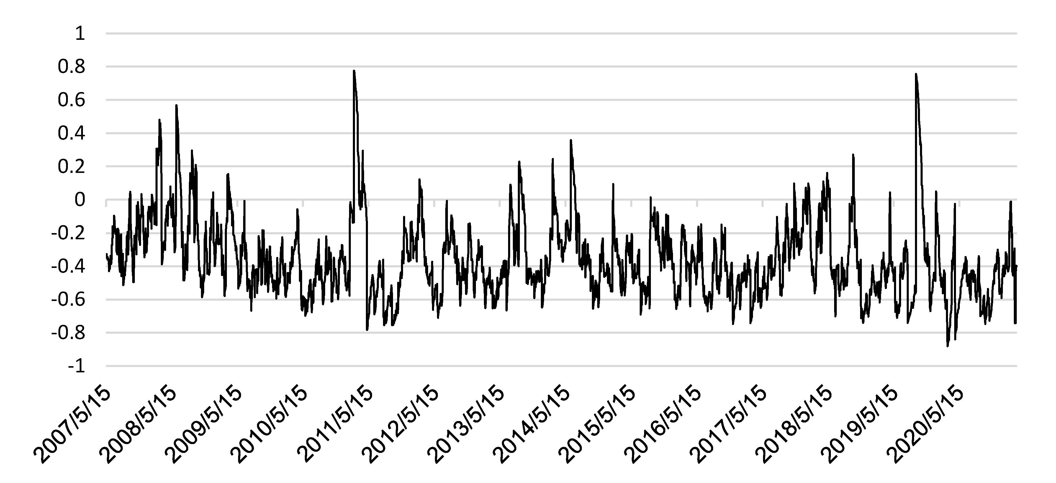
. We adopted the GJR-GARCH(1,1) model with skewed Student’s t-distribution to estimate the WTI oil return volatility. In the case of OVX changes the best model was the ARMA(1,1)-GARCH(1,1) with skewed Student’s t-distribution. The conditional correlation coefficient, shown in Figure 3, exhibits a time variation and presents a general negative dependence between WTI returns and OVX changes. Thus, when the oil price decreases the OVX index increases, while the oil price increases with OVX drop (Figure 1). An interesting fact is that during the GFC period the dependence was the weakest. The finding confirms that obtained from the static copula analysis. In the first period of GFC the oil price and OVX moved in the same direction, thus increasing their correlation. The interpretation of the dependence captured by the correlation coefficient does not hold for extreme changes. 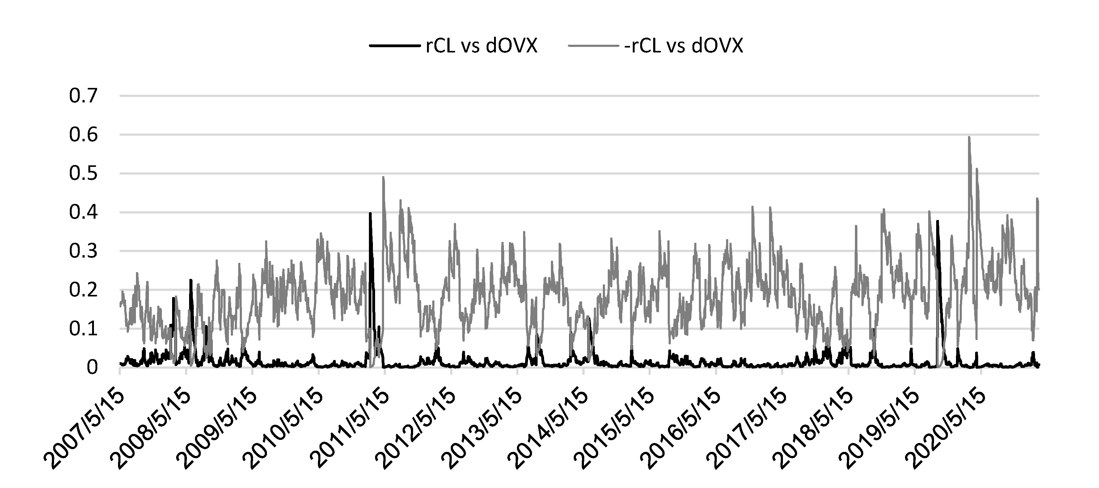The asymmetry between positive and negative returns in relation to OVX changes is easy to notice (Figure 4). The tail dependence between positive returns and OVX changes is approximately zero when excluding the isolated cases, indicating little or no dependence. However, for negative returns the dependence seems to maintain the high level and it reached level 0.6 in the COVID-19 crisis and the level 0.5 in the Arab Spring (the period of the uncertainty in oil supply stemming from the social instability in the Middle East and North Africa). The finding suggests that joint extreme movements of negative oil returns and OVX changes tended to occur most frequently during the COVID-19 crisis. In contrast, the lower tail dependence is observed in the GFC period.

4. Value at Risk Forecasting—Empirical Results

In this section we verify the usefulness of expectations towards oil prices, embedded in the implied volatility index OVX, to predict one-day ahead Value at Risk. As we found a tail dependence between OVX and crude oil returns, we expected that applying OVX could improve VaR forecasts for crude oil computed from the statistical model. As the VaR model we decided to use the conditional Extreme Value model (GARCH-EVT) proposed by McNeil and Frey [70]. The model guarantees high accuracy of risk estimations [70,71,72,73,74]. A GARCH-EVT approach is a two-stage hybrid method that combines a Generalized Autoregressive Conditional Heteroskedasticity (GARCH) filter with the Extreme Value Theory (EVT). In the first stage the GARCH approach is used to estimate empirical oil returns. In our study the GARCH(1,1) model is used:

$$r_t=\sqrt{h_t}{z}_t, h_t=\omega +\alpha r_{t-1}^2+\beta h_{t-1},$$

(29)

where: $\omega ,\alpha ,\beta >0, \alpha +\beta <1, z_t \sim \mathrm{i}.\mathrm{i}.\mathrm{d}.\left(0, 1\right); h_t$ represents conditional variance of $r_t$ and ${\widehat{z}}_t=r_t/\sqrt{{\widehat{h}}_t}$ are the standardized residuals. The GARCH-EVT-OVX model exploits the following volatility equation:

$$h_t=\omega +\alpha r_{t-1}^2+\beta h_{t-1}+\gamma {\sigma }_{OVX, t-1}^2,$$

(30)

where ${\sigma }_{OVX,t}$ denote the 1-day scaled implied volatility at time t.

In the second step the Peaks over Threshold (POT) method of EVT is applied to model the tails of standardized residues ${\widehat{z}}_t$ obtained from the GARCH model. The POT method is based on the Balkema–de Haan theorem [75], which states that exceedances (abnormal values of a random variable) y of a high threshold, u follow the Generalized Pareto Distribution (GPD) with CDF of the form:

$$G_{\xi ,\beta }\left(y\right)=\{\begin{array}{c}1-{\left(1+\xi \frac{y}{\beta }\right)}^{-\frac{1}{\xi }}, \xi \ne 0,\\ 1-\exp \left(-\frac{y}{\beta }\right), \xi =0,\end{array}$$

(31)

where $\xi \mathrm{and} \beta$ are distribution parameters which satisfy $\beta >0, y\ge 0$ for $\xi \ge 0$ and $0\le y\le -\frac{\beta }{\xi }$ for $\xi <0$. The q-quantile of GPD for sample size of length n is calculated as follows:

$$z_q=u+\frac{\widehat{\beta }}{\widehat{\xi }}\left({\left(\frac{1-q}{k/n}\right)}^{-\widehat{\xi }}-1\right),$$

(32)

where k is the number of exceedances of the threshold, u.

Using the POT approach requires to pre-specify the threshold, u which indicates the beginning of the upper distribution tail. The appropriate choice of a threshold level is a considerable challenge. A broad overview on how to choose the threshold may be found in [76,77,78,79]. The choice of the threshold in the GARCH-EVT model is discussed in [80]. The authors provide the rationale that the fixed threshold allows to produce VaRs with a similar accuracy as advanced optimization procedures. We set the 90th percentile as the threshold level in the empirical study, because such a selection of the threshold value enables the determination of VaR forecasts for the confidence levels of 95%, 97.5% and 99%. Moreover, for different threshold levels the GARCH-EVT model produces similar Value at Risk estimates [80].

The Value at Risk for a short position (right tail) in the GARCH-EVT model is calculated with the formula:

$$Va{R}_q^{t+1}=\sqrt{{\widehat{h}}_{t+1}} z_q,$$

(33)

where: ${\widehat{h}}_{t+1}$—one step ahead forecast of conditional volatility, $z_q$—GPD quantile calculated for the standardized residuals ${\widehat{z}}_t$ of the GARCH(1,1) model.

To test the forecasting performance of examined VaR models we used rolling windows of 504 returns and computed the VaR forecasts for each moving window. To evaluate the accuracy of forecasts we applied four different backtesting procedures, i.e., the Kupiec failure test, UC [81], the conditional coverage Christoffersen’s test, CC [82], the duration Christoffersen and Pelletier’s test, UD [83] and the dynamic quantile Engle and Manganelli’s test, DQ (the test included constant, VaR, first five lagged exceedances and one lagged squared return) [84]. These tests focus on exceedances of VaR forecasts by actual returns and consider it as a violation. The Kupiec test checks the valuation number, whereas the other tests evaluate their independence. An evaluation of the test size for small samples may be found in [85]. Laporta et al. [30] used a similar set of tests (Kupiec test, Christoffersen’s test, and Engle and Manganelli’s test) to assess VaR forecasts for daily returns on energy commodities. Marimoutou et al. [71] applied the loss function proposed by Lopez [86] as an additional measure of VaR forecasts for returns on WTI and Brent. Furthermore, as goodness-of-fit measures we present mean/maximum absolute deviation between the returns and the quantiles when the valuation occurs ADmean/ADmax used by McAleer and Da Veiga [87] and the loss function Q described by Gonzalez-Rivera et al. [88].

Table 6. Backtesting for VaRs based on the GARCH-EVT.

Quantile	ET	T1	UC	CC	UD	DQ	ADmean	Loss	T1	UC	CC	UD	DQ	ADmean	Loss
			p	p	p	p	ADmax			p	p	p	p	ADmax
		Panel A: Left tail for entire period							Panel B: Right tail for entire period
0.95	149	147	0.039	0.048	0.230	5.959	3.354	0.368	143	0.288	0.292	1.030	7.217	1.237	0.251
			0.843	0.976	0.632	0.652	292.494			0.591	0.864	0.310	0.513	16.058
0.975	74	72	0.099	0.484	1.134	0.642	5.603	0.266	65	1.344	4.237	0.007	1.321	1.503	0.150
			0.752	0.785	0.287	1.000	288.081			0.246	0.120	0.936	0.995	13.641
0.99	29	37	1.598	2.091	5.068	2.002	9.233	0.185	23	1.733	2.090	0.750	1.582	2.339	0.078
			0.206	0.352	0.024	0.981	281.978			0.188	0.352	0.387	0.991	10.264
		Panel C: Left tail for pre-COVID-19 period							Panel D: Right tail for pre-COVID-19 period
0.95	132	131	0.023	0.396	0.081	9.849	1.105	0.223	123	0.764	1.069	0.108	20.044	1.069	0.208
			0.879	0.820	0.776	0.276	7.757			0.382	0.586	0.743	0.010	11.580
0.975	66	62	0.299	3.218	0.932	14.839	1.266	0.134	53	2.956	5.117	0.048	19.414	1.344	0.123
			0.585	0.200	0.334	0.062	7.209			0.086	0.077	0.826	0.013	10.976
0.99	26	31	0.718	1.451	3.553	20.319	1.272	0.067	20	1.779	2.083	1.394	7.813	2.139	0.064
			0.397	0.484	0.059	0.009	6.531			0.182	0.353	0.238	0.452	10.264
		Panel E: Left tail for COVID-19 period							Panel F: Right tail for COVID-19 period
0.95	16	16	0.027	1.591	0.596	0.725	21.763	1.521	20	0.668	3.234	9.643	1.300	2.270	0.587
			0.869	0.451	0.440	0.999	292.494			0.414	0.198	0.002	0.996	16.058
0.975	8	10	0.325	1.432	0.157	0.821	32.491	1.314	12	1.467	2.367	4.866	1.369	2.205	0.364
			0.569	0.489	0.692	0.999	288.081			0.226	0.306	0.027	0.995	13.641
0.99	3	6	1.747	4.694	1.504	2.614	50.364	1.123	3	0.034	0.089	1.410	0.086	3.674	0.187
			0.186	0.096	0.220	0.956	281.978			0.853	0.957	0.235	1.000	9.864

Note: ET (T₁)—expected (actual) number of exceedances, UC—Kupiec test statistic, CC—Christoffersen’s test statistic, UD—Christoffersen and Pelletier’s test statistic, DQ—Engle and Manganelli’s test statistic (the DQ test included constant, VaR, first five lagged exceedances and one lagged squared return), p—p-value, ADmean (ADmax)—mean (maximum) absolute deviation between the returns and the quantiles if exceedances occur [87], Loss—loss function Q [88], bold—rejection of the null hypothesis at the significance level of 0.05. The calculations were performed with the rugarch and GAS packages in R [89,90].

shows the results of calculations for the GARCH-EVT model. Panels A and B present findings for the full research period, panels C and D for the pre-COVID-19 sample (from May 2007 to the end of November 2019) and panels E and F for the COVID-19 one. All calculations were made for long (left tail) and short (right tail) investors’ positions. The rejection of the null hypothesis at the 5% significance level is marked in bold and thus a failure of the VaR model. The Kupiec test confirms that the number of valuations is consistent with the expected one. However, the other tests display a dependence of VaR valuations. The duration UD test shows the existence of memory between VaR valuations in the right tail in the pandemic period (q = 97.5%, 95%) and in the left tail in the entire period (q = 99%). The dynamic quantile DQ test indicates that the current valuation is not independent on past processed information available in valuations, VaR and squared return. Based on the DQ test a dependence was found only in the pre-COVID-19 period in the right tail for q = 97.5%, 95% and in the left one for q = 99%. The goodness-of-fit measures, i.e., ADmean, ADmax and the loss function, take higher values for the left tail than for the right one indicating greater difficulties in risk measurement during crude oil price drops.

Comparing the results included in Table 6 and

Table 7. Backtesting for VaRs based on the GARCH-EVT with implied volatility.

Quantile	ET	T1	UC	CC	UD	DQ	ADmean	Loss	T1	UC	CC	UD	DQ	ADmean	Loss
			p	p	p	p	ADmax			p	p	p	p	ADmax
		Panel A: Left tail for entire period							Panel B: Right tail for entire period
0.95	149	146	0.080	0.291	0.789	4.198	3.375	0.368	141	0.500	0.519	0.864	5.922	1.242	0.251
			0.778	0.865	0.072	0.839	292.494			0.479	0.771	0.353	0.656	16.342
0.975	74	72	0.099	0.484	0.786	0.624	5.625	0.266	62	2.340	4.969	0.120	2.216	1.567	0.150
			0.752	0.785	0.375	1.000	288.081			0.126	0.083	0.729	0.974	13.980
0.99	29	37	1.598	2.091	6.487	1.984	9.258	0.185	23	1.733	2.090	0.750	1.582	2.339	0.078
			0.206	0.352	0.011	0.981	281.978			0.188	0.352	0.387	0.991	10.399
		Panel C: Left tail for pre-COVID-19 period							Panel D: Right tail for pre-COVID-19 period
0.95	132	130	0.058	1.129	0.003	8.051	1.114	0.224	121	1.118	1.523	0.060	20.237	1.074	0.208
			0.809	0.569	0.954	0.429	7.682			0.290	0.467	0.806	0.009	11.557
0.975	66	62	0.299	3.218	0.600	14.346	1.297	0.135	50	4.511	6.432	0.389	21.846	1.412	0.124
			0.585	0.200	0.439	0.073	7.115			0.034	0.040	0.533	0.005	10.941
0.99	26	32	1.065	1.846	4.544	19.970	1.258	0.067	20	1.779	2.083	1.394	7.818	2.112	0.064
			0.302	0.397	0.033	0.010	6.445			0.182	0.353	0.238	0.451	10.209
		Panel E: Left tail for COVID-19 period							Panel F: Right tail for COVID-19 period
0.95	16	16	0.027	1.591	0.596	0.725	21.763	1.521	20	0.668	3.234	9.643	1.300	2.270	0.587
			0.869	0.451	0.440	0.999	292.494			0.414	0.198	0.002	0.996	16.058
0.975	8	10	0.325	1.432	0.157	0.821	32.492	1.314	12	1.467	2.367	4.866	1.369	2.205	0.364
			0.569	0.489	0.692	0.999	288.081			0.226	0.306	0.027	0.995	13.641
0.99	3	6	1.747	4.694	1.504	2.614	50.364	1.123	3	0.034	0.089	1.410	0.086	3.674	0.187
			0.186	0.096	0.220	0.956	281.978			0.853	0.957	0.235	1.000	9.863

Note: ET (T₁)—expected (actual) number of exceedances, UC—Kupiec test statistic, CC—Christoffersen’s test statistic, UD—Christoffersen and Pelletier’s test statistic, DQ—Engle and Manganelli’s test statistic (the DQ test included constant, VaR, first five lagged exceedances and one lagged squared return), p—p-value, ADmean (ADmax)—mean (maximum) absolute deviation between the returns and the quantiles if exceedances occur [87], Loss—loss function Q [88], bold—rejection of the null hypothesis at the significance level of 0.05. The calculations were performed with the rugarch and GAS packages in R [89,90].

no significant differences were observed for the results of tests and goodness-of-fit measures. The number of valuations tends to be slightly lower for the model with implied volatility (Table 7). We can infer that the expectation factor does not improve the accuracy of forecasts received from the statistical model. This finding confirms these cited in the Introduction. Figure 5 shows the estimates of $\gamma$ in formula (30), which stands for the weight of the OVX in the volatility equation. The values of $\gamma$ are equal to zero for most of the research period. Only in periods of high volatility (the Arab Spring and COVID-19 periods) it is positive, although its value does not exceed 0.08. The impact of expectations in one-day ahead VaR forecasting seems to be negligible. This result may be explained by the tail co-movement between oil returns and OVX and a weak tail dependence between oil returns and lagged OVX. The concurrent reaction of extreme returns and OVX changes does not allow to take advantage the expectations in future risk assessment. Presumably, during an extended crisis time, when the tail dependence enhances the importance of the expectation factor in the volatility equation could play a greater role, but our research period does not allow to verify such a hypothesis.

5. Conclusions

The COVID-19 pandemic spread rapidly around the globe in 2020 and brought an unprecedented level of risk to the global oil market. The WTI oil price dropped to negative values driven by demand and supply factors. The new market conditions stimulated researchers to conduct empirical studies explaining various aspects of risk.

The research described in the paper examines the informative and predictive role of OVX. We study the tail dependence behavior of WTI oil returns and OVX changes. The unconditional and conditional copula approaches are applied in the empirical study. We found that negative oil price shocks depend on extreme OVX changes, whereas positive shocks and OVX changes are independent. The asymmetry in tail behavior convinces us that OVX behaves as a fear gauge for the oil market. The values of OVX increase rapidly during the turmoil in the oil market and are not vulnerable to the extreme oil price increases. As expected, the highest tail dependence is evidenced in the COVID-19 crisis. We provide the evidence that implied volatility is much more closely related to WTI oil price than ex-ante volatility calculated with the GARCH methodology. Moreover, in contrast to implied volatility the GARCH volatility is not asymmetrical in the relation to WTI oil returns. The information content of the two volatility types differs substantially.

To verify the usefulness of the OVX index in tail risk forecasting the two approaches are compared. The importance of the expectation factor (OVX) in crude oil volatility modeling and the VaR forecasting increases in the Arab Spring and the COVID-19 health crisis, but it does not play a significant role. Based on the back-testing procedures we could not confirm the ability of OVX to improve one day-ahead forecasts of the Value at Risk. The impact of investors’ expectations embedded in OVX on VaR forecasts seems to be negligible. The results of this study may be helpful for all investors, risk managers and academics who are interested in risk analysis for global energy market.

References

1. Belke, A.; Bordon, I.; Hendricks, T. Global liquidity and commodity prices—A cointegrated VAR approach for OECD countries. Appl. Financ. Econ. 2010, 20, 227–242. [Google Scholar] [CrossRef] [Green Version]
2. Ratti, R.A.; Vespignani, J.L. Oil prices and global factor macroeconomic variables. Energy Econ. 2016, 59, 198–212. [Google Scholar] [CrossRef] [Green Version]
3. Amendola, A.; Candila, V.; Scognamillo, A. On the influence of US monetary policy on crude oil price volatility. Empir. Econ. 2017, 52, 155–178. [Google Scholar] [CrossRef]
4. Yi, A.; Yang, M.; Li, Y. Macroeconomic Uncertainty and Crude Oil Futures Volatility—Evidence from China Crude Oil Futures Market. Front. Environ. Sci. 2021, 9, 636903. [Google Scholar] [CrossRef]
5. Ghassan, H.B.; AlHajhoj, H.R. Long run dynamic volatilities between OPEC and non-OPEC crude oil prices. Appl. Energy 2016, 169, 384–394. [Google Scholar] [CrossRef] [Green Version]
6. Liao, G.; Li, Z.; Du, Z.; Liu, Y. The Heterogeneous Interconnections between Supply or Demand Side and Oil Risks. Energies 2019, 12, 2226. [Google Scholar] [CrossRef] [Green Version]
7. Bildirici, M.; Guler Bayazit, N.; Ucan, Y. Analyzing Crude Oil Prices under the Impact of COVID-19 by Using LSTARGARCHLSTM. Energies 2020, 13, 2980. [Google Scholar] [CrossRef]
8. Engebretsen, R.; Anderson, C. The Impact of Coronavirus (COVID-19) and the Global Oil Price Shock on the Fiscal Position of oil-Exporting Developing Countries. OECD 2020, 1–18. Available online: https://www-oecd-org.ezproxy.uis.no/coronavirus/policy-responses/the-impact-of-coronavirus-covid-19-and-the-global-oil-price-shock-on-the-fiscal-position-of-oil-exporting-developing-countries-8bafbd95/%0Ahttps://www.oecd-ilibrary.org/development/developme (accessed on 12 May 2021).
9. Bouri, E.; Demirer, R.; Gupta, R.; Pierdzioch, C. Infectious Diseases, Market Uncertainty and Oil Market Volatility. Energies 2020, 13, 4090. [Google Scholar] [CrossRef]
10. Nyga-Łukaszewska, H.; Aruga, K. Energy Prices and COVID-Immunity: The Case of Crude Oil and Natural Gas Prices in the US and Japan. Energies 2020, 13, 6300. [Google Scholar] [CrossRef]
11. Wheeler, C.M.; Baffes, J.; Kabundi, A.N.; Kindberg-Hanlon, G.; Nagle, P.S.O.; Ohnsorge, F.L. Adding Fuel to the Fire: Cheap Oil during the COVID-19 Pandemic. In Policy Research Working Paper Series 9320; The World Bank: Washington, DC, USA, 2020; pp. 1–47. Available online: https://ideas.repec.org/p/wbk/wbrwps/9320.html (accessed on 23 June 2021).
12. De Blasis, R.; Petroni, F. Price Leadership and Volatility Linkages between Oil and Renewable Energy Firms during the COVID-19 Pandemic. Energies 2021, 14, 2608. [Google Scholar] [CrossRef]
13. Ji, Q.; Fan, Y. Modelling the joint dynamics of oil prices and investor fear gauge. Res. Int. Bus. Financ. 2016, 37, 242–251. [Google Scholar] [CrossRef]
14. Shaikh, I. The relation between implied volatility index and crude oil prices. Eng. Econ. 2019, 30, 556–566. [Google Scholar] [CrossRef] [Green Version]
15. Benedetto, F.; Mastroeni, L.; Quaresima, G.; Vellucci, P. Does OVX affect WTI and Brent oil spot variance? Evidence from an entropy analysis. Energy Econ. 2020, 89, 104815. [Google Scholar] [CrossRef]
16. Choi, S.Y.; Hong, C. Relationship between uncertainty in the oil and stock markets before and after the shale gas revolution: Evidence from the OVX, VIX, and VKOSPI volatility indices. PLoS ONE 2020, 15, e0232508. [Google Scholar] [CrossRef]
17. Maghyereh, A.I.; Awartani, B.; Bouri, E. The directional volatility connectedness between crude oil and equity markets: New evidence from implied volatility indexes. Energy Econ. 2016, 57, 78–93. [Google Scholar] [CrossRef] [Green Version]
18. Bašta, M.; Molnár, P. Oil market volatility and stock market volatility. Financ. Res. Lett. 2018, 26, 204–214. [Google Scholar] [CrossRef]
19. Dutta, A. Oil and energy sector stock markets: An analysis of implied volatility indexes. J. Multinatl. Financ. Manag. 2018, 44, 61–68. [Google Scholar] [CrossRef]
20. Liu, M.L.; Ji, Q.; Fan, Y. How does oil market uncertainty interact with other markets? An empirical analysis of implied volatility index. Energy 2013, 55, 860–868. [Google Scholar] [CrossRef]
21. Lin, J.B.; Tsai, W. The relations of oil price change with fear gauges in global political and economic environment. Energies 2019, 15, 2982. [Google Scholar] [CrossRef] [Green Version]
22. Lv, W. Does the OVX matter for volatility forecasting? Evidence from the crude oil market. Phys. A Stat. Mech. Appl. 2018, 492, 916–922. [Google Scholar] [CrossRef]
23. Antonakakis, N.; Chatziantoniou, I.; Filis, G. Dynamic spillovers of oil price shocks and economic policy uncertainty. Energy Econ. 2014, 44, 433–447. [Google Scholar] [CrossRef] [Green Version]
24. Chatziantoniou, I.; Degiannakis, S.; Delis, P.; Filis, G. Forecasting oil price volatility using spillover effects from uncertainty indices. Financ. Res. Lett. 2020, 101885. [Google Scholar] [CrossRef]
25. Chen, Y.; He, K.; Yu, L. The Information Content of OVX for Crude Oil Returns Analysis and Risk Measurement: Evidence from the Kalman Filter Model. Ann. Data Sci. 2015, 2, 471–487. [Google Scholar] [CrossRef] [Green Version]
26. Lin, J.B.; Liang, C.C.; Tsai, W. Nonlinear relationships between oil prices and implied volatilities: Providing more valuable information. Sustainability 2019, 11, 3906. [Google Scholar] [CrossRef] [Green Version]
27. Liu, B.Y.; Ji, Q.; Fan, Y. Dynamic return-volatility dependence and risk measure of CoVaR in the oil market: A time-varying mixed copula model. Energy Econ. 2017, 68, 53–65. [Google Scholar] [CrossRef]
28. Agbeyegbe, T.D. An inverted U-shaped crude oil price return-implied volatility relationship. Rev. Financ. Econ. 2015, 27, 28–45. [Google Scholar] [CrossRef]
29. Chen, Y.; Zou, Y. Examination on the relationship between OVX and crude oil price with Kalman filter. Procedia Comput. Sci. 2015, 55, 1359–1365. [Google Scholar] [CrossRef] [Green Version]
30. Laporta, A.G.; Merlo, L.; Petrella, L. Selection of Value at Risk Models for Energy Commodities. Energy Econ. 2018, 74, 628–643. [Google Scholar] [CrossRef]
31. Lian, Z.; Cai, J.; Webb, R.I. Oil stocks, risk factors, and tail behavior. Energy Econ. 2020, 91, 104932. [Google Scholar] [CrossRef]
32. Peña, J.I.; Rodríguez, R.; Mayoral, S. Tail risk of electricity futures. Energy Econ. 2020, 91, 104886. [Google Scholar] [CrossRef]
33. Poon, S.; Rockinger, M.; Tawn, J. Extreme value dependence in financial markets: Diagnostics, models, and financial implications. Rev. Financ. Stud. 2003, 17, 581–610. [Google Scholar] [CrossRef]
34. De Jonghe, O. Back to the basics in banking? A micro-analysis of banking system stability. J. Financ. Intermed. 2010, 19, 387–417. [Google Scholar] [CrossRef] [Green Version]
35. Longin, F.; Solnik, B. Extreme correlation of international equity markets. J. Financ. 2001, 56, 649–676. [Google Scholar] [CrossRef]
36. Harvey, C.; Siddique, A. Conditional skewness in asset pricing tests. J. Financ. 2000, 55, 1263–1295. [Google Scholar] [CrossRef]
37. Dittmar, R. Nonlinear pricing kernels, kurtosis preference, and evidence from the cross section of equity returns. J. Financ. 2002, 57, 369–403. [Google Scholar] [CrossRef]
38. Hill, B. A simple general approach to inference about the tail of a distribution. Ann. Stat. 1975, 3, 1163–1174. [Google Scholar] [CrossRef]
39. Kelly, B.; Jiang, H. Tail risk and asset prices. Rev. Financ. Stud. 2014, 27, 2841–2871. [Google Scholar] [CrossRef] [Green Version]
40. Van Ordt, M.; Zhou, C. Systematic tail risk. J. Financ. Quant. Anal. 2016, 51, 685–705. [Google Scholar] [CrossRef]
41. Adrian, T.; Brunnermeier, M. CoVaR. Am. Econ. Rev. 2016, 106, 1705–1741. [Google Scholar] [CrossRef]
42. Shehzad, K.; Zaman, U.; Liu, X.; Górecki, J.; Pugnetti, C. Examining the Asymmetric Impact of COVID-19 Pandemic and Global Financial Crisis on Dow Jones and Oil Price Shock. Sustainability 2021, 13, 4688. [Google Scholar] [CrossRef]
43. Christoffersen, P.; Hahn, J.; Inoue, A. Testing and comparing value-at-risk measures. J. Empir. Financ. 2001, 8, 325–342. [Google Scholar] [CrossRef] [Green Version]
44. Chong, J. Value at risk from econometric models and implied from currency options. J. Forecast. 2004, 23, 603–620. [Google Scholar] [CrossRef]
45. Kim, J.S.; Ryu, D. Are the KOSPI 200 implied volatilities useful in value-at-risk models? Emerg. Mark. Rev. 2015, 22, 43–64. [Google Scholar] [CrossRef]
46. Bongiovanni, A.; De Vincentii, P.; Isaia, E. The VIX Index: Forecasting Power and Performance in a Risk Management Framework. J. Financ. Manag. Mark. Inst. 2016, 2, 129–144. [Google Scholar]
47. Giot, P. Implied volatility indexes and daily value at risk models. J. Deriv. 2005, 12, 54–64. [Google Scholar] [CrossRef]
48. Bali, T.G.; Weinbaum, D. A conditional extreme value volatility estimator based on high-frequency returns. J. Econ. Dyn. Control. 2007, 31, 361–397. [Google Scholar] [CrossRef]
49. Fueki, T.; Nakajima, J.; Ohyama, S.; Tamanyu, Y. Identifying oil price shocks and their consequences: The role of expectations in the crude oil market. Int. Financ. 2020, 24, 53–76. [Google Scholar] [CrossRef]
50. Sklar, A. Fonctions de Répartition à n Dimensions et Leurs Marges. Publ. Inst. Stat. Univ. Paris 1959, 8, 229–231. [Google Scholar]
51. Aas, K. Pair-copula constructions for financial applications: A review. Econometrics 2016, 4, 43. [Google Scholar] [CrossRef] [Green Version]
52. Nelsen, R.B. An Introduction to Copulas, 1st ed.; Springer Series in Statistics: New York, NY, USA, 2007. [Google Scholar]
53. Cherubini, U.; Luciano, E.; Vecchiato, W. Copula Methods in Finance; John Wiley & Sons Inc: New York, NY, USA, 2013. [Google Scholar]
54. Trivedi, P.K.; Zimmer, D.M. Copula modeling: An introduction for practitioners. Found Trends Econom. 2005, 1, 1–111. [Google Scholar] [CrossRef] [Green Version]
55. Aloui, R.; Hammoudeh, S.; Nguyen, D.K. A time-varying copula approach to oil and stock market dependence: The case of transition economies. Energy Econ. 2013, 39, 208–221. [Google Scholar] [CrossRef]
56. Patton, A.J. Modelling asymmetric exchange rate dependence. Int. Econ. Rev. 2006, 47, 527–556. [Google Scholar] [CrossRef]
57. Jondeau, E.; Rockinger, M. The Copula-GARCH model of conditional dependencies: An international stock market application. J. Int. Money Financ. 2006, 25, 827–853. [Google Scholar] [CrossRef] [Green Version]
58. Patton, A.J. Copula-based models for financial time series. In Handbook of Financial Time Series; Andersen, T.G., Davis, R.A., Kreiss, J.-P., Mikosch, T., Eds.; Springer: New York, NY, USA, 2009; pp. 767–786. [Google Scholar]
59. Bollerslev, T. Generalized autoregressive conditional heteroskedasticity. J. Econom. 1986, 31, 307–327. [Google Scholar] [CrossRef] [Green Version]
60. Tsay, R.S. Analysis of Financial Time Series; John Willey & Sons: New York, NY, USA, 2005. [Google Scholar]
61. Fałdziński, M.; Fiszeder, P.; Orzeszko, W. Forecasting Volatility of Energy Commodities: Comparison of GARCH Models with Support Vector Regression. Energies 2020, 14, 6. [Google Scholar] [CrossRef]
62. Salisu, A.A.; Fasanya, I.O. Modelling oil price volatility with structural breaks. Energy Policy. 2013, 52, 554–562. [Google Scholar] [CrossRef]
63. Nelson, D.B. Conditional Heteroskedasticity in Asset Returns: A New Approach. Econometrica 1991, 2, 347–370. [Google Scholar] [CrossRef]
64. Glosten, L.R.; Jagannathan, R.; Runkle, D.E. On the Relation between the Expected Value and the Volatility of the Nominal Excess Return on Stocks. J. Financ. 1993, 4, 899–905. [Google Scholar] [CrossRef]
65. Ding, Z.; Granger, C.W.J.; Engle, R.F. A long memory property of stock market returns and a new model. J. Empir. Financ. 1993, 1, 83–106. [Google Scholar] [CrossRef]
66. Engle, R.F. Dynamic conditional correlation: A simple class of multivariate generalized autoregressive conditional heteroskedasticity models. J. Bus. Econ. Stat. 2002, 20, 339–350. [Google Scholar] [CrossRef]
67. Aielli, G.P. Dynamic Conditional Correlation: On Properties and Estimation. J. Bus. Econ. Stat. 2013, 31, 282–299. [Google Scholar] [CrossRef]
68. Echaust, K. Asymmetric tail dependence between stock market returns and implied volatility. J. Econ. Asymmetries 2021, 23, 1–13. [Google Scholar] [CrossRef]
69. Genest, C.; Rémillard, B.; Beaudoin, D. Goodness-of-fit tests for copulas: A review and a power study. Insur. Math. Econ. 2009, 44, 199–213. [Google Scholar] [CrossRef]
70. McNeil, A.J.; Frey, R. Estimation of tail-related risk measures for heteroscedastic financial time series: An extreme value approach. J. Empir. Financ. 2000, 7, 271–300. [Google Scholar] [CrossRef]
71. Marimoutou, V.; Raggad, B.; Trabelsi, A. Extreme Value Theory and Value at Risk: Application to oil market. Energy Econ. 2009, 4, 519–530. [Google Scholar] [CrossRef] [Green Version]
72. Echaust, K.; Just, M. A Comparison of Conditional and Unconditional VaR Models. Proc. Int. Sci. Conf. Hradec Econ. Days 2020 2020, 10, 124–135. [Google Scholar]
73. Youssef, M.; Belkacem, L.; Mokni, K. Value-at-Risk estimation of energy commodities: A long-memory GARCH-EVT approach. Energy Econ. 2015, 51, 99–110. [Google Scholar] [CrossRef]
74. Li, L. Comparative Study of GARCH and EVT Model in Modeling Value-at-Risk. J. Appl. Bus. Econ. 2017, 19, 27–48. [Google Scholar]
75. Balkema, A.A.; De Haan, L. Residual life time at great age. Ann. Probab. 1974, 2, 792–804. [Google Scholar] [CrossRef]
76. Just, M.; Echaust, K. An Optimal Tail Selection in Risk Measurement. Risks 2021, 4, 1–16. [Google Scholar]
77. Danielsson, J.; Ergun, L.; de Haan, L.; de Vries, C. Tail Index Estimation: Quantile Driven Threshold Selection; London Sch Econ Polit Sci: London, UK, 2016; p. 58. [Google Scholar]
78. Caeiro, F.; Gomes, M.I. Threshold selection in extreme value analysis. In Extreme Value Modeling and Risk Analysis: Methods and Applications; Dipak, K.D., Jun, Y., Eds.; Chapman and Hall/CRC: New York, NY, USA, 2016; pp. 69–86. [Google Scholar]
79. Scarrott, C.; MacDonald, A. A review of extreme value threshold estimation and uncertainty quantification. Revstat Stat. J. 2012, 10, 33–60. [Google Scholar]
80. Echaust, K.; Just, M. Value at risk estimation using the GARCH-EVT approach with optimal tail selection. Mathematics 2020, 8, 114. [Google Scholar] [CrossRef] [Green Version]
81. Kupiec, P.H. Techniques for Verifying the Accuracy of Risk Measurement Models. J. Deriv. 1995, 3, 73–84. [Google Scholar] [CrossRef]
82. Christoffersen, P.F. Evaluating Interval Forecasts. Int. Econ. Rev. 1998, 39, 841–862. [Google Scholar] [CrossRef]
83. Christoffersen, P.F.; Pelletier, D. Backtesting Value-at-Risk: A Duration-Based Approach. J. Financ. Econom. 2004, 2, 84–108. [Google Scholar] [CrossRef]
84. Engle, R.F.; Manganelli, S. CAViaR: Conditional autoregressive value at risk by regression quantiles. J. Bus. Econ. Stat. 2004, 22, 367–381. [Google Scholar] [CrossRef]
85. Kaszyński, D.; Kamiński, B.; Pankratz, B. Assessment of the size of VaR backtests for small samples. Przegląd Stat. 2020, 67, 114–151. [Google Scholar] [CrossRef]
86. Lopez, J.A. Testing your risk tests. Financ. Surv. 1998, May–June, 18–20. [Google Scholar]
87. McAleer, M.; Da Veiga, B. Forecasting value-at-risk with a parsimonious Portfolio Spillover GARCH (PS-GARCH) model. J. Forecast. 2008, 27, 1–19. [Google Scholar] [CrossRef] [Green Version]
88. González-Rivera, G.; Lee, T.H.; Mishra, S. Forecasting volatility: A reality check based on option pricing, utility function, value-at-risk, and predictive likelihood. Int. J. Forecast. 2004, 20, 629–645. [Google Scholar] [CrossRef]
89. Ghalanos, A. Rugach: Univariate GARCH Models, R Package, Version 1.4-4. 2020. Available online: https://cran.r-project.org/web/packages/rugarch/index.html (accessed on 15 February 2021).
90. Catania, L.; Boudt, K.; Ardia, D. GAS: Generalized Autoregressive Score Models, R package, Version 0.3.3. 2020. Available online: https://cran.r-project.org/web/packages/GAS/index.html (accessed on 15 February 2021).
Figure 1. Crude Oil Future Contract—CLF (USD per barrel) and CBOE Crude Oil Volatility Index—OVX in 11 May 2007–30 March 2021.
Energies 14 04147 g001
Figure 2. Common exceedances of extreme values. The left panel shows all data, the right panel data without outliers. Note: Extreme values mean exceedances of the 5th and 95th quantiles of Crude Oil Future Contract returns (rCL) and the 95th quantile of changes in the CBOE Crude Oil Volatility Index (dOVX), and in volatility (dVOL).
Energies 14 04147 g002
Figure 3. Estimation of the conditional correlation coefficient for the relationship between Crude Oil Future Contract returns (rCL) and changes in the CBOE Crude Oil Volatility Index (dOVX) in the entire period.
Energies 14 04147 g003
Figure 4. Estimation of the tail dependence coefficient for the relationship between Crude Oil Future Contract returns (rCL)/negative returns (−rCL) and changes in the CBOE Crude Oil Volatility Index (dOVX) in the entire period.
Energies 14 04147 g004
Figure 5. Estimates of the gamma parameter in formula (30) for a moving window of size 504.
Energies 14 04147 g005