Application of Dynamic Fault Tree Analysis to Prioritize Electric Power Systems in Nuclear Power Plants

Abstract

Because the scope of risk assessments at nuclear power plants (NPPs) is being extended both spatially and temporally, conventional, or static fault trees might not be able to express failure mechanisms, or they could be unnecessarily conservative in their expression. Therefore, realistic assessment techniques are needed to adequately capture accident scenarios. In multi-unit probabilistic safety assessment (PSA), fault trees naturally become more complex as the number of units increases. In particular, when considering a shared facility between units of the electric power system (EPS), static fault trees (SFTs) that prioritize a specific unit are limited in implementing interactions between units. However, dynamic fault trees (DFTs) can be available without this limitation by using dynamic gates. Therefore, this study implements SFTs and DFTs for an EPS of two virtual NPPs and compares their results. In addition, to demonstrate the dynamic characteristics of the shared facilities, a station blackout (SBO), which causes the power system to lose its function, is assumed—especially with an inter-unit shared facility, AAC DG (Alternate AC Diesel Generator). To properly model the dynamic characteristics of the shared EPS in DFTs, a modified dynamic gate and algorithm are introduced, and a Monte Carlo simulation is adopted to quantify the DFT models. Through the analysis of the DFT, it is possible to confirm the actual connection priority of AAC DG according to the situation of units in a site. In addition, it is confirmed that some conservative results presented by the SFT can be evaluated from a more realistic perspective by reflecting this.

1. Introduction

The systems and components of nuclear power plants (NPPs) should be evaluated to predict and prepare for potential failures. Probabilistic safety assessments (PSAs) are one commonly used method. Since the Fukushima Daiichi accident in Japan showed that multiple units within a site could be simultaneously exposed to risk, multi-unit PSAs have been studied [1]. For a system under certain conditions, such as activation or failure of preceding equipment, an arrangement of operating or failure times of components may have a significant impact on the entire system. When performing a multi-unit PSA in Korea, this is prominently displayed in the electric power system (EPS). Therefore, when the time arrangement of components is identified, it is expected that it could be possible to contribute to further complementing a system model by securing new combinations of failure of components that have not been previously checked and producing realistic results.

Although conventional event trees and fault trees have often been deemed sufficient in presenting outcomes that fit the purpose of a PSA, they are unavoidably conservative because of the difficulty in identifying the behavior of components over time. In other words, conventional event trees and fault trees do not reflect the dynamic effects of failure timing, the sequence of failing components, or system and operator actions during a failure. In particular, because traditional fault trees apply only to general linear systems, they cannot adequately address the dynamic characteristics of a failure over time, such as dependencies and interactions among components [2]. Despite those limitations, the conventional methods are still useful. However, because the scope of risk assessments at NPPs is being extended both spatially and temporally, conventional, or static fault trees might not be able to express particular failure mechanisms, or they could be unnecessarily conservative in their expression. Furthermore, in multi-unit PSA, this issue becomes more prominent as it deals with more complex problems as the number of units increases.

Those shortcomings could be met by using a dynamic PSA, which enables the identification of plant behavior over time and can be performed using dynamic event trees and dynamic fault trees (DFTs) in a context similar to a conventional PSA. The dynamic PSA can, thus, implement realistic models of plant systems by identifying new paths to system success depending on dynamic behavior. From the viewpoint of modeling system or component failure, DFTs can be implemented by introducing dynamic gates into conventional fault trees to consider the redundancy, failure complexes, and recovery times of the systems [3]. Examples of application to a system using these dynamic gates have also been presented in previous studies [3,4].

Several methods have been proposed to capture dynamic system behavior, ranging from Markov models to DFTs [5,6]. A Markov chain allows the conversion of components’ states to reflect the concept of time in a Markov model, determining the probability of a top event. However, it has difficulty in determining the correct Markov model for a given system. To circumvent that trouble, DFTs were introduced, and many researchers have proposed methods for solving them. Using a Markov chain to solve dynamic gates created problems, such as a state space explosion when the number of input data increase, high time requirements, and inconsistent models [7,8]. The state space explosion is particularly problematic for PSAs of NPPs, which deal with a huge number of cutsets [9]. Therefore, various researchers have attempted to compensate for that limitation. A methodology for building a Markov model by modularizing each independent substructure was suggested, but it still faces the state space explosion problem [10]. A numerical integration method was also proposed, but it cannot easily be applied to repairable systems [11]. Nevertheless, software that solves DFT by integrating these methods has also been developed, such as DIFTree [12,13]. A Monte Carlo simulation, which solves DFTs without the limitations of a Markov chain and has advantages in simulating actual processes and random behavior in systems, has been successfully and practically adopted in software, such as DRSIM and MatCarlore [14]. Bayesian networks also enable fast and accurate calculations [15]. Analyses using binary decision diagrams and fuzzy theory methods are also available [16,17].

This study uses a DFT to identify the dynamic characteristics of a system in a certain situation. In Korea, two or more units generally share an alternative AC diesel generator (AAC DG), which can become an issue in the case of a multi-unit station blackout (SBO). For this purpose, multi-unit PSA studies ranging from two or four units [18,19] to six or more units [20] have been performed. The AAC DG is included in the EPS of an NPP and is available on only one train of one unit. In other words, when the AAC DG is connected to one of the units that share it, electric power cannot be recovered in the other units, which will inevitably lead to core damage [21]. However, in the fault tree models of a multi-unit PSA, the shared AAC DG is usually assumed to connect preferentially to a specific unit [22]. Although the number of AAC DGs is steadily increasing, so that each unit can be matched to an AAC DG as needed, it is currently difficult to determine the priority of connection between units in a multi-unit accident. Therefore, this paper simulates the EPSs of two virtual NPPs to reflect a dual-unit SBO situation using an SFT and DFT and then compare the results. Furthermore, it introduces a method for implementing dynamic characteristics in SFTs and DFTs and presents newly developed algorithms and additional conditional expressions for dynamic gates to quantify the given DFT in particular conditions. AIMS-PSA software was used to construct and quantify the SFTs [23], and the DFTs were implemented by coding directly. To quantify dynamic gates for the DFT, a Monte Carlo simulation approach was chosen to determine the near accurate values with simulation results and secure as many as possible for a specific situation, and only non-repairable devices were considered. Throughout this study, conventional fault trees are called SFTs to distinguish them from DFTs.

This paper is organized as follows: Section 2 describes the modeling process and reflects the characteristics of each fault tree in a dual-unit SBO. Section 2.1 covers the structure of the EPSs in the two virtual NPPs, and Section 2.2 introduces the reliability data, and assumptions of the SFT implemented. The features of each dynamic gate that forms the DFT and a method for quantifying them are presented in Section 2.3.1 and Section 2.3.2. Section 2.3.3 describes a situation that cannot be solved by the existing dynamic gate alone, due to the characteristics of EPS. The DFT built on that basis is presented in Section 2.3.4, and additional conditional expressions for the dynamic gate developed to reflect the limitations of the AAC DG are also described here. Section 3 then presents the results from the developed SFTs and DFTs and compares their determination of the priorities for the AAC DG. Related discussion and conclusions are given in Section 4.

2. Methodology Development

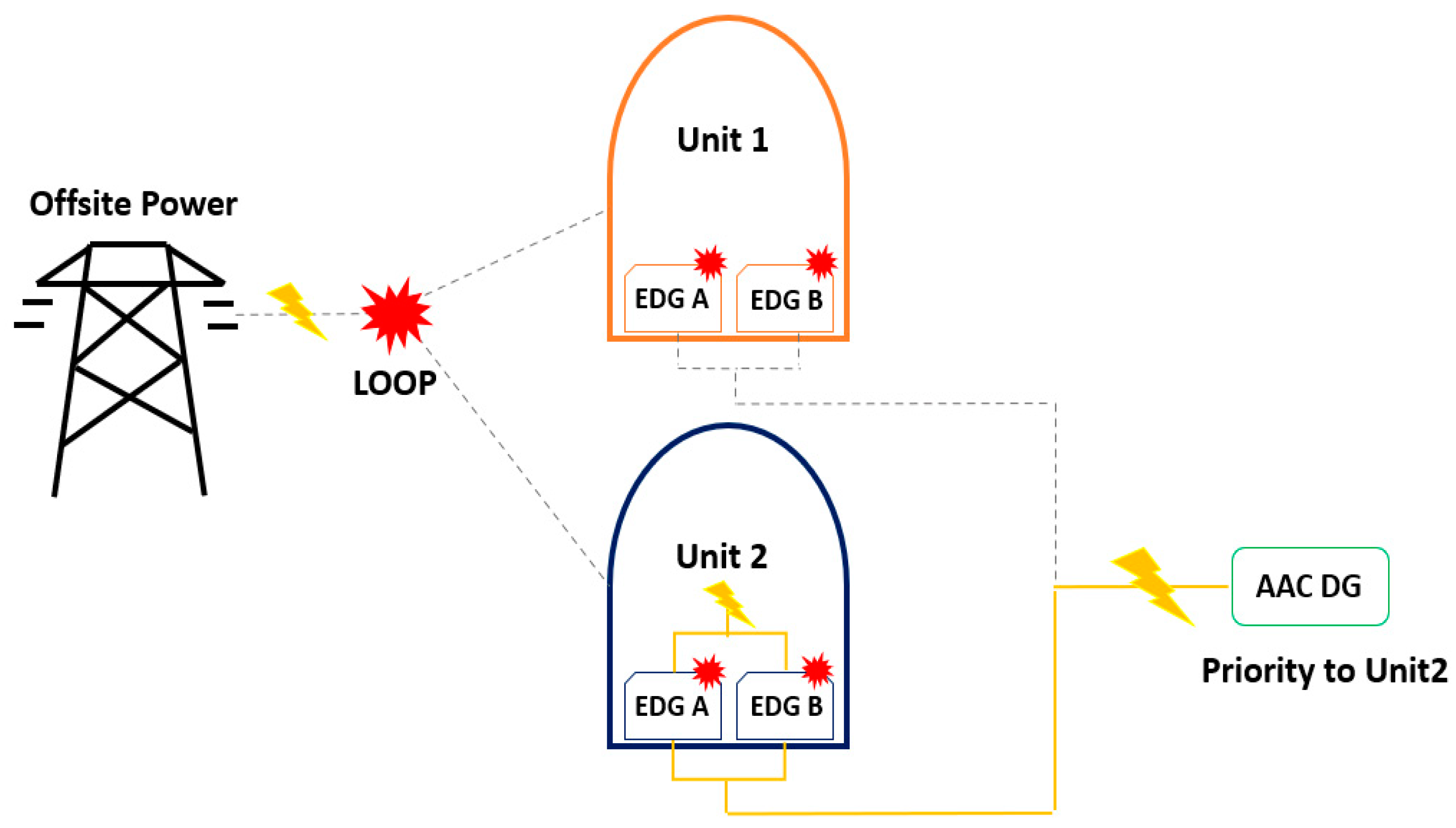
2.1. EPS Structure

The EPS is a supporting system that supplies electric power to all the components and systems in an NPP. In normal operation, the plant transmits the electric power it generates to the outside, and it receives the electricity required for its operation from an offsite power source. Furthermore, the power is depressurized through transformers to match the rated voltage of the plant components and then supplied to each power bus line. In the EPS structure, all bus lines with upper to lower voltages are connected, and each bus line is divided into A and B trains [20]. In addition, each train is designed to recover power using an emergency diesel generator (EDG) in the event of a loss of offsite power (LOOP). If the EDG fails or is otherwise unavailable, the plant enters an SBO situation and gets a supply of power through the AAC DG, an inter-unit shared facility on site [24]. In other words, the AAC DG is only used when both EDGs connected to each train are unavailable. However, a multi-unit SBO, when several units simultaneously need the AAC DG, could still occur if all the EDGs in multiple units fail at the same time. Furthermore, because an AAC DG can be connected to only one train in a single unit, it is difficult to determine the priority between units, as shown in Figure 1.

On this issue, this paper compares an SFT constructed with the assumption that priority is given to a specific train of a certain unit with a DFT that reflects AAC DG availability according to dynamic interactions. For this purpose, the EPS of generally pressurized water reactor was configured in a simple form to show the dynamic characteristics well. For the convenience of description in the following, the target plant that suffers the top event in the fault trees will be called Unit 1, and its neighboring plant on the same site is called Unit 2.

Figure 2 shows a simplified single line diagram (SLD) of the EPS for the dual unit, indicating that each unit has access to offsite power, 4.16 kV bus lines, EDGs, and the AAC DG. It is assumed that the offsite power is supplied to both units and connected to trains A and B of the 4.16 kV buses. In addition, each unit has two EDGs that can be connected to either train, and the AAC DG is assumed to be capable of connecting to any train in either unit. This EPS was prepared simply for the purpose of this study; the actual composition would vary depending on the research purpose or actual situation in a plant.

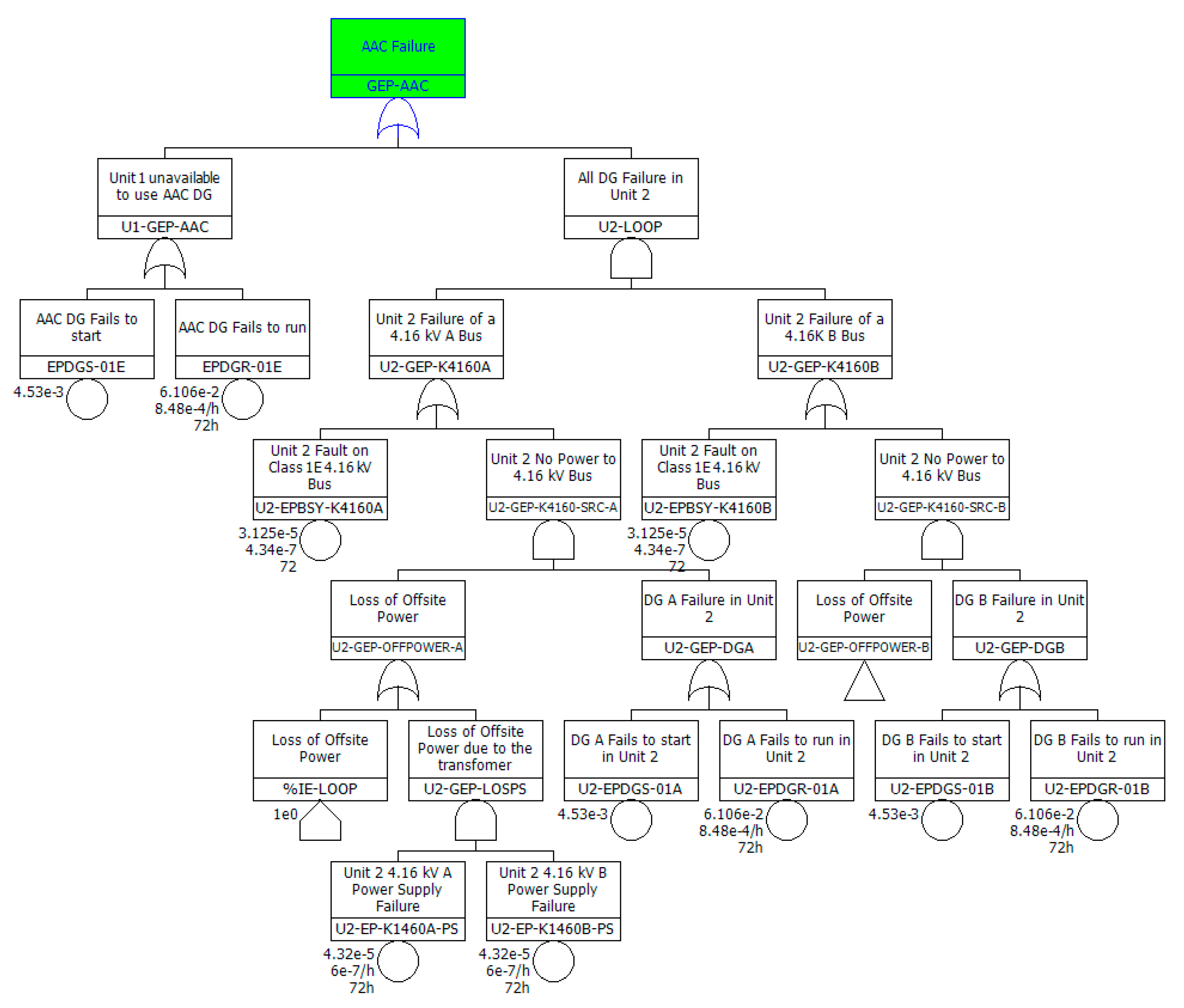
2.2. Static Fault Tree Analysis

In this study, both an SFT and DFT are evaluated by targeting Unit 1. Therefore, the top event in the fault trees produces a failure to supply power to all trains in Unit 1. The following considerations were applied to construct the SFT of the EPS.

• It is assumed that 4.16 kV is the offsite power.
• Failure to run to the supply power, and failure of the bus are considered for each 4.16 kV A/B bus.
• Batteries and lower voltage buses are not considered.
• A LOOP accident is taken as the initiating event with the probability one.
• Standby failure, failure to start, and failure to run are considered for EDG A/B and the AAC DG.
• Only part of the EPS in Unit 2 is considered.
• Unavailable to use AAC DG in Unit 1 is considered to accommodate a failure of EDG A/B in Unit 2 (only for SFT).

An SFT cannot model dynamic interactions, but it can determine whether the AAC DG is available to Unit 1 according to the operation status of the EPS in Unit 2. In other words, Unit 1 cannot use the AAC DG if Unit 2 requires it (i.e., both EDGs in Unit 2 are unavailable). Generic data were used in both the SFT and DFT and are presented in

Table 1. Reliability data for constructing the SFT and DFT.

Event Name	Description	Failure Mode	Failure Rate (h−1)	Mission Time (h)
%IE-LOOP	Loss of Offsite Power	Demand	1
EPBSY-K4160B	Fault on Class 1E 4.16 kV Bus in Unit 1	Running	$4.34\times {10}^{-07}$	72
EPBSY-K4160A	Fault on Class 1E 4.16 kV Bus in Unit 1	Running	$4.34\times {10}^{-07}$	72
EP-K1460A-PS	4.16 kV A Power Supply Failure in Unit 1	Running	$6.00\times {10}^{-07}$	72
EP-K1460B-PS	4.16 kV B Power Supply Failure in Unit 1	Running	$6.00\times {10}^{-07}$	72
EPDGS-01A	EDG A Fails To Start in Unit 1	Demand	$4.53\times {10}^{-07}$
EPDGS-01B	EDG B Fails To Start in Unit 1	Demand	$4.53\times {10}^{-07}$
EPDGS-01E	AAC DG Fails To Start	Demand	$4.53\times {10}^{-07}$
EPDGR-01A	EDG A Fails To Run in Unit 1	Running	$8.48\times {10}^{-07}$	72
EPDGR-01B	EDG B Fails To Run in Unit 1	Running	$8.48\times {10}^{-07}$	72
EPDGR-01E	AAC DG Fails To Run	Running	$8.48\times {10}^{-07}$	72
U2-EPBSY-K4160A	Fault on Class 1E 4.16 kV Bus in Unit 2	Running	$4.34\times {10}^{-07}$	72
U2-EPBSY-K4160B	Fault on Class 1E 4.16 kV Bus in Unit 2	Running	$4.34\times {10}^{-07}$	72
U2-EP-K1460A-PS	4.16 kV A Power Supply Failure in Unit 2	Running	$6.00\times {10}^{-07}$	72
U2-EP-K1460B-PS	4.16 kV B Power Supply Failure in Unit 2	Running	$6.00\times {10}^{-07}$	72
U2-EPDGS-01A	EDG A Fails To Start in Unit 2	Demand	$4.53\times {10}^{-07}$
U2-EPDGS-01B	EDG B Fails To Start in Unit 2	Demand	$4.53\times {10}^{-07}$
U2-EPDGR-01A	EDG A Fails To Run in Unit 2	Running	$8.48\times {10}^{-07}$	72
U2-EPDGR-01B	EDG B Fails To Run in Unit 2	Running	$8.48\times {10}^{-07}$	72

[25].

Figure 3 and Figure 4 show part of the SFT for the EPS using the SLD and considerations and the reliability data. Figure 4 stands for the transferred AAC DG failure gate (GEP-AAC) in Figure 3. The SFTs in the figures are for the A train of Unit 1, and the B train has a symmetrical structure. AIMS-PSA software was used to implement this SFT [23].

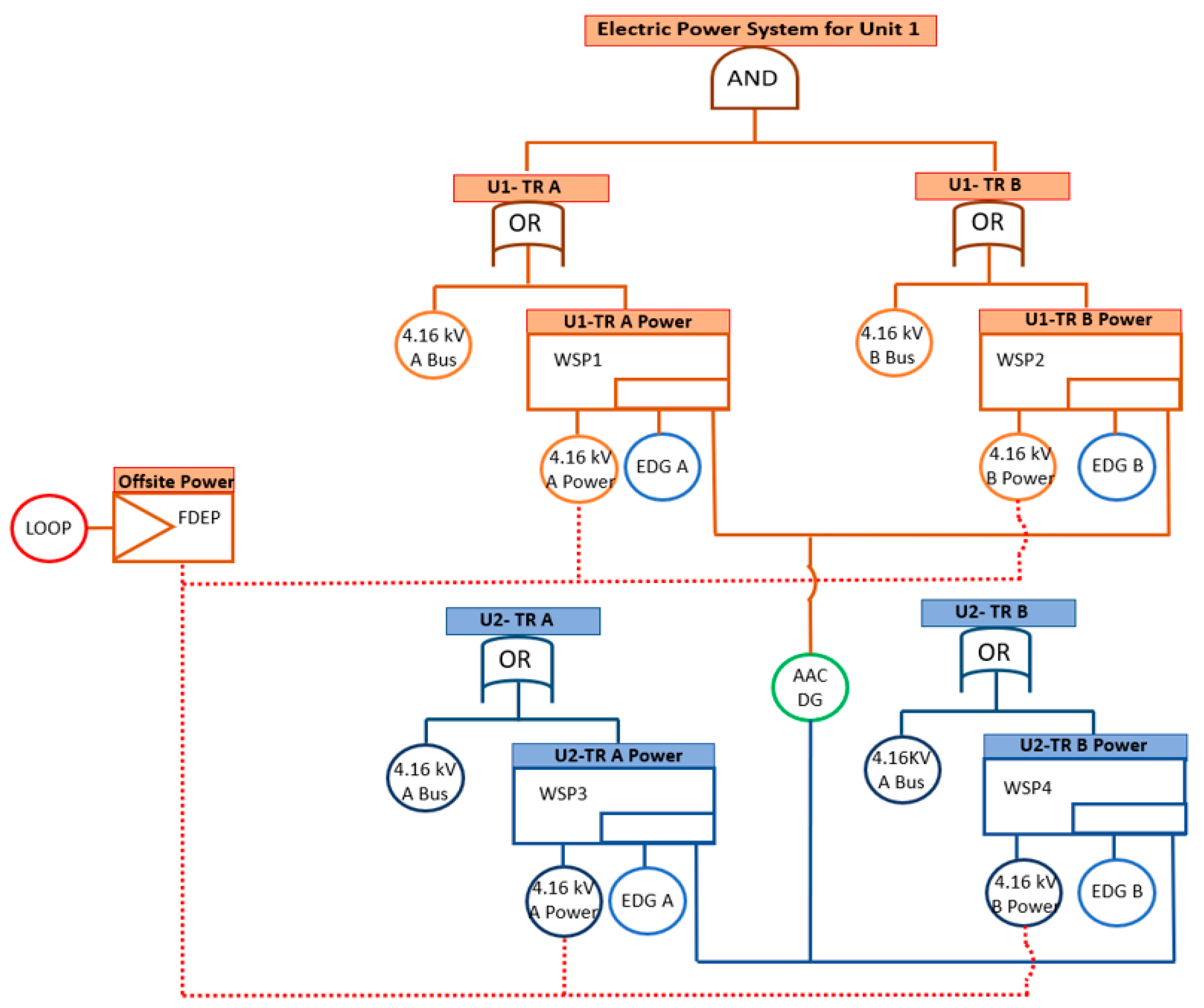
2.3. Dynamic Fault Tree Analysis

2.3.1. Characteristics of a Dynamic Fault Tree

A DFT is a method for adding dynamic gates that deal with sequential concepts to an SFT. With the help of dynamic gates, modelers can specify sequence-dependent system failure behavior, spares, and dynamic redundancy management. Furthermore, priorities during a failure event are compact and easily understood in DFTs [3]. They can also consider combinations that can change the failure state of a system by implementing a component’s startup, shutdown, and repair within a mission time.

In this study, the Monte Carlo simulation approach was used to quantify the DFTs. The Monte Carlo simulation is mainly used to represent the aleatory uncertainty which is related to the stochastic distribution of the physical parameters in models [16]. The key in using the Monte Carlo simulation method is to generate random numbers to determine the failure timing and failure sequence. The failure rate of each component in the system is assigned to a basic event, and most of the reliability analysis addresses only random failures, which have a constant instantaneous failure rate $\lambda$ at time $t$ that follows the exponential distribution, as given in Equation (1) [9].

$$t=G\left(F\left(t\right)\right)=\frac{1}{\lambda }ln\left(\frac{1}{1-F\left(t\right)}\right)$$

(1)

where $F\left(t\right)$ is a random number with a uniform distribution generated in $\left[0,1\right]$. If $t$ is smaller than the mission time, the component is considered to have failed. If the components have a fixed probability, representing a demand failure, it can be expressed as given in Equation (2) [14].

$$t=\{\begin{array}{c}\infty if q\ge {\lambda }_d\\ t_q if q<{\lambda }_d\end{array}$$

(2)

where ${\lambda }_d$ is a demand failure, q is a random number with a uniform distribution in $\left[0,1\right]$, and $t_q$ is a random number generated uniformly between 0 and the mission time.

The failure time of the components derived using those equations is the input for the basic event that constitutes a dynamic gate, enabling the calculation of the unreliability of the top event in a way that reflects the dynamic interactions among components in the system.

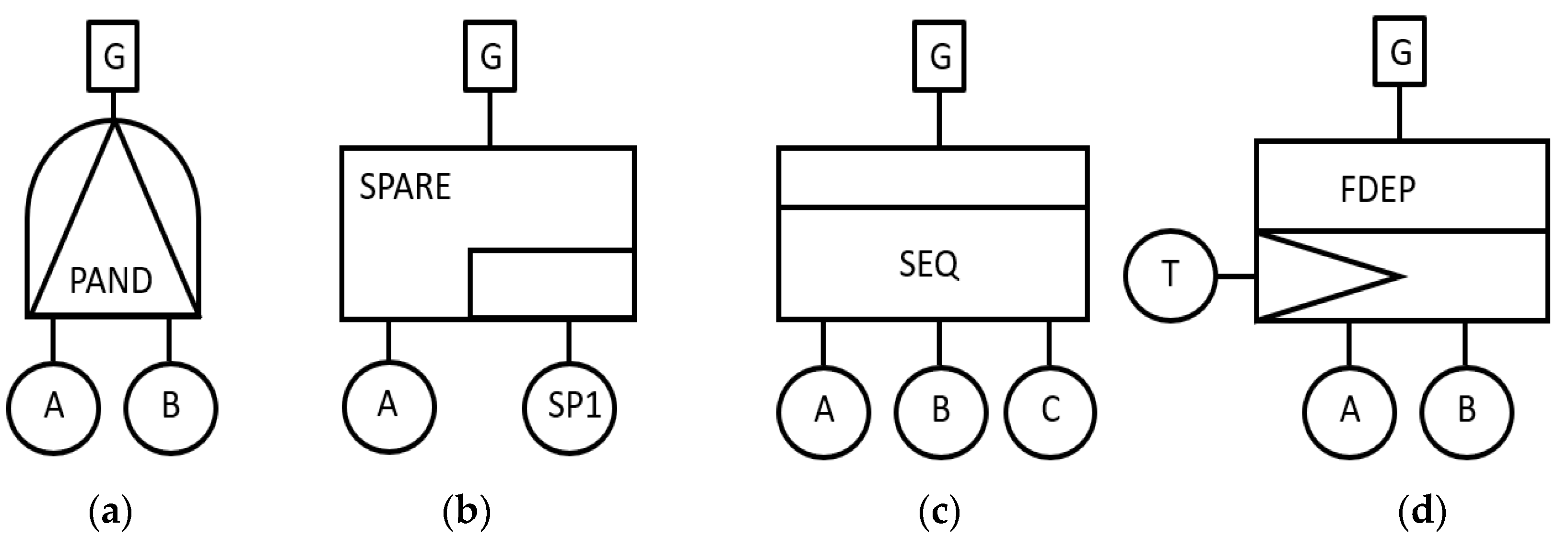
2.3.2. Dynamic Gates

The four dynamic gates that constitute DFTs are shown in Figure 5 [6]. Generalized formulas for each dynamic gate that can be used in a spreadsheet were presented in a previous study [26]. In this section, we briefly explain the characteristics of and output derivation formulas for each dynamic gate.

The priority AND (PAND) gate is similar to an AND gate, but its output depends on a basic event on the left (A) occurring before an event on the right (B). Therefore, logical expressions for deriving the output of the PAND gate can be represented, as shown in

Table 2. Logical expression for deriving the output of a PAND gate.

Gate	$\mathbf{Time} \mathbf{of} \mathbf{Failure} \left({\mathit{T}}_{\mathit{i}}\right)$	$\mathbf{State} \left({\mathit{S}}_{\mathit{i}}\right)$
PAND	$T_{PAND}\leftarrow \mathrm{IF}(\mathrm{AND}(T_A<T_B, T_B<T_M)$, $T_B, \infty )$	$S_{PAND}\leftarrow \mathrm{IF}(T_{PAND}<T_M), 1, 0)$

. In other words, the failure time of B ($T_B)$ is considered as an output of gate only when it is smaller than the mission time ($T_M)$ and larger than the failure time of A ($T_A)$, otherwise the gate provides an output with an infinite failure time ($\infty )$. If the failure time of the gate $(T_{PAND})$ is also greater than $T_M$, the gate is deemed a failure, and its output state is denoted as 1.

The standby or spare (SPARE) gate reflects extra components ($S_1$) that can replace the failed component with the same functionality. The SPARE gate fails when the failure time of the number of components, including spares, is less than the minimum required. Standby components can fail even when they are dormant, which can be expressed as a dormancy factor, $\alpha$, where $0\le \alpha \le 1$. Therefore, a SPARE gate can be cold $\left(\alpha =0\right)$, warm $(0<\alpha <1)$, or hot $\left(\alpha =1\right)$, depending on the dormancy factor [11]. In addition, the failure time for a spare component in the standby state can be considered the same as that calculated using its startup failure rate.

Table 3. Logical expression for deriving the output of a SPARE gate.

Component	$\mathbf{Time} \mathbf{of} \mathbf{Failure} \left({\mathit{T}}_{\mathit{i}}\right)$	$\mathbf{State} \left({\mathit{S}}_{\mathit{i}}\right)$
SP1-SB (Stand By)	$T_{SP1-SB}$	$S_{SP1-SB}\leftarrow$ $\mathrm{IF}\left(\mathrm{AND}\left(T_{SP1-SB}<T_M, T_{SP1-SB}<T_A\right), 1, 0\right)$
SP1-AC (Active)	$T_{SP1-AC}\leftarrow$ $(1-S_{SP1-SB}$)*$T_{SP1-AC}$	$S_{SP1-AC}\leftarrow \mathrm{IF}(\mathrm{AND}(T_{SP1-AC}<T_M), 1, 0)$
Gate	Time of Failure ($T_i$)	State ($S_i$)
SPARE	$T_{SPARE}\leftarrow T_A+T_{SP1-AC}$	$S_{SPARE}\leftarrow \mathrm{IF}(T_{SPARE}<T_M, 1, 0)$

presents logical expressions that produce the output of a SPARE gate that reflects the standby failure of a single spare component. The first line is to determine whether a failure of the spare component occurs while it is waiting $(S_{SP1-SB}=1$). It compares whether the failure time of the spare in the standby state ($T_{SP1-SB}$) is less than the failure time of the running component ($T_A$) and $T_M$. The next line calculates the total failure time of the spare. If $S_{SP1-SB}=1$, the failure time, including the operation of the spare $(T_{SP1-AC}$) becomes zero. Therefore, the final failure time of the SPARE gate ($T_{SPARE})$ is the sum of $T_A$ and $T_{SP1-AC}$, and the state of the gate $(S_{SPARE})$ is settled by comparing that time with $T_M.$

A sequence enforcing (SEQ) gate forces its inputs to fail in a particular order, and those inputs never happen in a different order. Ab SEQ gate can also be considered as a Cold-SPARE (CSP) gate.

Table 4. Logical expression for deriving the output of an SEQ gate.

Gate	$\mathbf{Time} \mathbf{of} \mathbf{Failure} \left({\mathit{T}}_{\mathit{i}}\right)$	$\mathbf{State} \left({\mathit{S}}_{\mathit{i}}\right)$
SEQ	$T_{SEQ}\leftarrow T_A+T_B+T_{\mathrm{C}}$	$S_{SEQ}\leftarrow \mathrm{IF}(T_{SEQ}<T_M), 1, 0)$

gives an expression for computing an SEQ gate, where the sum of the failure times for the three components ($T_A$, $T_B$, $T_{\mathrm{C}})$ becomes the final failure time. Like the other gates, the state of the output is compared with $T_M$. This study did not use SEQ or PAND gates to implement the DFT.

The functional dependency (FDEP) gate has a trigger event that forces dependent events to occur. Therefore, the FDEP gate has no output, but it can determine the state of dependent events.

Table 5. Logical expression for deriving the output of an FDEP gate.

Component	$\mathbf{Time} \mathbf{of} \mathbf{Failure} \left({\mathit{T}}_{\mathit{i}}\right)$	$\mathbf{State} \left({\mathit{S}}_{\mathit{i}}\right)$
A	$T_A\leftarrow MIN\left(T_T,T_A\right)$	$S_A\leftarrow \mathrm{IF}(T_A<T_M), 1, 0)$
B	$T_B\leftarrow MIN\left(T_T,T_B\right)$	$S_B\leftarrow \mathrm{IF}(T_B<T_M), 1, 0)$

shows expressions for calculating the components of an FDEP gate. The dependent events determine their own states when the minimum (MIN) failure time between the trigger ($T_T$) and dependent events ($T_A$, $T_B$) is smaller than $T_M$. The failure time expression of a dependent event is the same as with an OR gate, and the expression for an AND gate can be given by using the maximum failure time between events instead of the minimum.

2.3.3. Development of Dynamic Gate for a Specific Shared Facility

In an NPP, a component can be shared within a system or between systems. In those cases, a dynamic gate can be expressed in the form of two SPARE gates that share one redundant component, as shown in Figure 6.

In general, because the shared spare is used by the side that fails first, it is easy to determine the available priority. The expressions for calculating SPARE gates for this case were discussed in a previous study, as shown in

Table 6. Logical expression for deriving the output of two SPARE gates that share one component.

Component	Additional Condition 1 (AC1)	Additional Condition 2 (AC2)
SP1-SB for SPARE Gate 1 (Standby)	$\mathrm{AC}1\leftarrow \mathrm{IF}\left(\mathrm{AND}\left(T_{SP1-SB}<T_M, T_{SP1-SB}<T_A\right), 1, 0\right)$	$\mathrm{AC}2\leftarrow \mathrm{IF}(T_A<T_B, 1, 0)$
SP1-SB for SPARE Gate 2 (Standby)	$\mathrm{AC}1\leftarrow \mathrm{IF}(\mathrm{AND}(T_{SP1-SB}<T_M, T_{SP1-SB}<T_B), 1, 0)$	$\mathrm{AC}2\leftarrow \mathrm{IF}(T_B<T_A, 1, 0)$
Gate	Time of Failure (Ti)	State (Si)
SPARE 1 (Spare-Active)	$T_{SPARE 1}\leftarrow \mathrm{MAX}\left(T_A, \left(T_A+T_{SP1-AC}\right)\ast AC1\ast AC2\right)$	$S_{SPARE 1}\leftarrow$ $\mathrm{IF}(T_{SPARE 1}<T_M, 1, 0)$
SPARE 2 (Spare-Active)	$T_{SPARE 2}\leftarrow \mathrm{MAX}\left(T_B, \left(T_B+T_{SP1-AC}\right)\ast AC1\ast AC2\right)$	$S_{SPARE 2}\leftarrow$ $\mathrm{IF}(T_{SPARE 2}<T_M, 1, 0)$

[26].

Some additional conditional expressions are required to solve these gates. The first additional condition is the same as the expression for determining the presence or absence of a failed spare in the standby state of a single SPARE gate. The second additional condition determines a SPARE gate in which the components in the operating state ($T_A,T_B)$ fail first. In other words, the spare component finds the required gate in a faster time. Therefore, each SPARE gate has a failure time relevant to the shared component through the discrimination state value of those two conditions. However, the above expressions cannot be used if other specific conditions are required to run the shared component, for example, when a spare component is activated only when all operating components have stopped. This is one of the characteristics that appeared in the process of constructing the DFT for the EPS. For example, the EDGs are activated when both trains are unavailable, due to LOOP, and the AAC DG operates only when both EDGs are lost. Therefore, more additional conditional expressions are required to solve dynamic gates that reflect those conditions. How to solve a SPARE gate that includes a shared component with a specific operating condition will be described in the next section.

2.3.4. Construction of the Dynamic Fault Tree

The DFT used in this study reflects all the considerations and reliability data addressed in the SFT. To implement the DFT targeted in this study, it was necessary to distinguish the priority for the spare using the dynamic interactions among components. Figure 7 shows the DFT of the EPS constructed for this study.

The top event of the DFT is the failure to supply power to all trains in Unit 1, which is the same as for the SFT in Section 2.2. In this DFT, the two SPARE gates on the upper side indicate components within Unit 1, and those on the lower side represent components within Unit 2. If each high-voltage 4.16 kV bus fails, the trains in both units are left without power, despite the additional power systems. Because the 4.16 kV power is supplied from an offsite power source, LOOP and the power of all trains can configure the FDEP gate as a trigger and dependent event, respectively. The EDGs, which support each train when LOOP occurs, are the first spare on all the SPARE gates, and the AAC DG is the second spare that can be shared among all trains on both units. In addition, this study implemented Warm-SPARE (WSP) gates by computing the failure time using the startup failure rate to consider failures in the standby state for all spares.

Gates other than the SPARE gates can be solved using the expressions explained in Section 2.3.2. Therefore, this section provides additional conditional expressions and solutions that reflect the characteristics of the EPS to clarify the SPARE gates. The unusual aspects of the EPS that are to be addressed by the SPARE gates are described in detail in

Table 7. Logical expressions for the SPARE gate to supply power to train A in Unit 1 following dual-unit LOOP.

Component	Time to Failure (Ti)	State (Si)
EDG A-SB (Standby)	$T_{EDGA1-SB}$	$S_{EDGA1-SB}\leftarrow$ $\mathrm{IF}(\mathrm{AND}(T_{EDGA1-SB}<T_M,T_{EDGA1-SB}<T_{4.16 A1}), 1, 0)$
EDG A-AC (Active)	$T_{EDGA1-AC}\leftarrow (1-S_{EDGA1-SB}$)*$T_{EDGA1-AC}$	$S_{EDGA1-AC}\leftarrow \mathrm{IF}(\mathrm{AND}(T_{EDGA1-AC}<T_M), 1, 0)$
Component	Additional Condition for EDG
EDG A for Train A	$A{C}_{EDG}\leftarrow \mathrm{IF}(\mathrm{NOT}(\mathrm{AND}(T_{4.16A1}<T_M, T_{4.16B1}<T_M), 0, 1)$ =$IF(\mathrm{MAX}(T_{4.16A1}, T_{4.16B1})<T_M, 1, 0)$
Gate	Time to Failure (Ti)	State (Si)
SPARE Train A with EDG (AC)	$T_{4.16A1+EDGA1}\leftarrow T_{4.16A1}+(A{C}_{EDG}\ast T_{EDGA1-AC})$	$S_{4.16A1+EDGA1}\leftarrow \mathrm{IF}(T_{4.16A1+EDGA1}<T_M, 1, 0)$
Component	Time to Failure (Ti)	State (Si)
AAC DG-SB (Standby)	$T_{AAC-SB}$	$S_{AAC-SB}\leftarrow$ $\mathrm{IF}(\mathrm{AND}(T_{AAC-SB}<T_M,$ $T_{AAC-SB}<T_{4.16A1+EDGA1}+T_{4.16B1+EDGB1}), 1, 0)$
AAC DG-AC (Active)	$T_{AAC-AC}\leftarrow (1-S_{AAC-SB}$)*$T_{AAC-AC}$	$S_{AAC-AC}\leftarrow \mathrm{IF}(\mathrm{AND}(T_{AAC-AC}<T_M), 1, 0)$
Component	Additional Conditions for AAC DG
AAC DG for Train A (AC1)	$AC1\leftarrow \mathrm{IF}\left(\mathrm{AND}\left(T_{AAC-SB}<T_M, T_{AAC-SB}<T_{4.16A1+EDGA1}\right), 0, 1\right)$
AAC DG for Train A (AC2)	$AC2\leftarrow IF(AND(T_{4.16A1+EDGA1}<T_{4.16B1+EDGB1},1,0)$
AAC DG for Train A (AC3)	$AC3\leftarrow \mathrm{IF}(\mathrm{NOT}(\mathrm{AND}(T_{4.16A1+EDGA1}<T_M, T_{4.16B1+EDGB1}<T_M), 0, 1)$ = $IF(MAX(T_{4.16A1+EDGA1}, T_{4.16B1+EDGB1})<T_M, 1, 0)$
AAC DG for Train A (AC4)	$AC4\leftarrow IF(MAX(T_{4.16A1+EDGA1}, T_{4.16B1+EDGB1})<MAX(T_{4.16A2+EDGA2}, T_{4.16B2+EDGB2}), 1, 0)$
Gate	Time to Failure (Ti)	State (Si)
SPARE Train A with EDG and AAC DG	$T_{TRA1}\leftarrow T_{4.16A1+EDGA1}+$ ($T_{AAC-AC}\ast AC1\ast AC2\ast AC3\ast AC4)$	$S_{TRA1}\leftarrow \mathrm{IF}(T_{TRA1}<T_M, 1, 0)$

. Take, for example, the process of deciding whether to connect the AAC DG to train A in Unit 1 after dual-unit LOOP has occurred.

In the case of EDG A, because a WSP gate is used, the total failure time ($T_{EDGA1-AC})$ is calculated by considering the failure of EDG A in standby ($T_{EDGA1-SB})$, as shown in Table 3. In addition, an additional condition $(A{C}_{EDG}$) for the EDG judges whether a lack of offsite power to both the 4.16 kV buses (A and B) should be considered. Therefore, if the failure time of the power supplied to 4.16 kV buses A and B ($T_{4.16A1}$, $T_{4.16B1}$) does not reach the mission time ($T_M$), EDG A in Unit 1 is started, and the failure time reflecting the first spare $\left(T_{4.16A1+EDGA1}\right)$ can be derived. In that way, it is possible to produce the failure time while considering the EDGs for all remaining trains $(T_{4.16B1+EDGB1}$, $T_{4.16A2+EDGA2}$, $T_{4.16B2+EDGB2})$. The AAC DG can also fail in the dormant state, and the standby time lasts until all of the EDGs for each unit fail. However, for train A of Unit 1 to use the AAC DG, four additional conditions must be met. The first additional condition (AC1) is that the standby time of the AAC DG ($T_{AAC-SB}$) must be longer than the sum of the operating times of offsite power and the EDG ($T_{4.16A1+EDGA1}$). The second additional condition (AC2) checks the priority between trains A and B in Unit 1, which confirms whether train A ($T_{4.16A1+EDGA1}$) is disabled before B ($T_{4.16B1+EDGB1}$). The third additional condition (AC3) identifies whether both EDG A and B have failed before $T_M$ to determine whether the AAC DG should be connected (i.e., judgement of an SBO). The last condition (AC4) reflects the characteristic of an inter-unit shared facility that is unavailable to the remaining units if the AAC DG is already in use, due to an earlier failure time in Unit 2 ($T_{4.16A2+EDGA2}$, $T_{4.16B2+EDGB2}$). With those conditions, it is possible to derive the failure time and status of the SPARE gate for the power supply to train A of Unit 1 ($T_{TRA1})$, and the same procedure can be applied to the other SPARE gates.

3. Results and Discussion

3.1. Static Fault Tree Evaluation

When the SFT presented in Section 2.2 was quantified, the unavailable frequency of the EPS for Unit 1 in a dual-unit LOOP was 3$.108\times {10}^{-04}$.

Table 8. The top 30 cutsets presented by AIMS-PSA software as the result of the SFT.

Group	No.	Basic Event 1	Basic Event 2	Basic Event 3	Basic Event 4	Basic Event 5
Ⅰ	1	%IE-LOOP	EPDGR-01A	EPDGR-01B	EPDGR-01E
	2	%IE-LOOP	EPDGR-01A	EPDGR-01B	EPDGS-01E
	3	%IE-LOOP	EPDGR-01A	EPDGR-01E	EPDGS-01B
	4	%IE-LOOP	EPDGR-01B	EPDGR-01E	EPDGS-01A
	5	%IE-LOOP	EPDGR-01E	EPDGS-01A	EPDGS-01B
	6	%IE-LOOP	EPDGR-01A	EPDGS-01B	EPDGS-01E
	7	%IE-LOOP	EPDGR-01B	EPDGS-01A	EPDGS-01E
	8	%IE-LOOP	EPBSY-K4160B	EPDGR-01A	EPDGR-01E
	9	%IE-LOOP	EPBSY-K4160A	EPDGR-01B	EPDGR-01E
	10	%IE-LOOP	EPDGS-01A	EPDGS-01B	EPDGS-01E
	11	%IE-LOOP	EPBSY-K4160B	EPDGR-01A	EPDGS-01E
	12	%IE-LOOP	EPBSY-K4160A	EPDGR-01B	EPDGS-01E
	13	%IE-LOOP	EPBSY-K4160A	EPDGR-01E	EPDGS-01B
	14	%IE-LOOP	EPBSY-K4160B	EPDGR-01E	EPDGS-01A
Ⅱ	15	%IE-LOOP	EPDGR-01A	EPDGR-01B	U2-EPDGR-01A	U2-EPDGR-01B
	16	%IE-LOOP	EPDGR-01B	EPDGS-01A	U2-EPDGR-01A	U2-EPDGR-01B
	17	%IE-LOOP	EPDGR-01A	EPDGS-01B	U2-EPDGR-01A	U2-EPDGR-01B
	18	%IE-LOOP	EPDGR-01A	EPDGR-01B	U2-EPDGR-01B	U2-EPDGS-01A
	19	%IE-LOOP	EPDGR-01A	EPDGR-01B	U2-EPDGR-01A	U2-EPDGS-01B
	20	%IE-LOOP	EPDGS-01A	EPDGS-01B	U2-EPDGR-01A	U2-EPDGR-01B
	21	%IE-LOOP	EPDGR-01A	EPDGS-01B	U2-EPDGR-01A	U2-EPDGS-01B
	22	%IE-LOOP	EPDGR-01B	EPDGS-01A	U2-EPDGR-01B	U2-EPDGS-01A
	23	%IE-LOOP	EPDGR-01B	EPDGS-01A	U2-EPDGR-01A	U2-EPDGS-01B
	24	%IE-LOOP	EPDGR-01A	EPDGS-01B	U2-EPDGR-01B	U2-EPDGS-01A
	25	%IE-LOOP	EPDGR-01A	EPDGR-01B	U2-EPDGS-01A	U2-EPDGS-01B
	26	%IE-LOOP	EPDGR-01A	EPDGR-01B	U2-EPBSY-K4160A	U2-EPDGR-01B
	27	%IE-LOOP	EPBSY-K4160B	EPDGR-01A	U2-EPDGR-01A	U2-EPDGR-01B
	28	%IE-LOOP	EPBSY-K4160A	EPDGR-01B	U2-EPDGR-01A	U2-EPDGR-01B
	29	%IE-LOOP	EPDGR-01A	EPDGR-01B	U2-EPBSY-K4160B	U2-EPDGR-01A
	30	%IE-LOOP	EPDGS-01A	EPDGS-01B	U2-EPDGR-01B	U2-EPDGS-01A

shows the top 30 cutsets calculated using the SFT, with each cutset composed of the event names, shown in Table 1.

Each cutset represents a combination of equipment failures that cause EPS unavailability in Unit 1, and becomes a comparison target for the DFT results presented in the next section. The first cutset occupies the largest probability of space as an accident in which even the AAC DG fails in an SBO situation in which both EDGs A and B failed during operation, as shown in Figure 8. In addition, most of the cutsets in the upper ranks consist of a combination of startup and running failures of the EDGs and AAC DG after LOOP. These types of cutsets are marked as group Ⅰ. However, those cutsets do not show the order of failure for trains A and B in Unit 1, so even if the AAC DG is available, it is not possible to determine which train connects to the AAC DG. Furthermore, the situation of Unit 2 is also unknown. Some of the cutsets produced after the fourteenth cutset and marked as group Ⅱ contain an accident by which the EDGs are unavailable for both Units 1 and 2, as shown in Figure 9. As suggested as a limitation of the SFT model, this can be understood because of transferring the priority of the AAC DG to Unit 2 when all the EDGs in Unit 2 are unavailable. In other words, because the AAC DG is being used by Unit 2, it is marked as an accident in the cutsets of the SFT that target Unit 1. However, even in that case, the order of train failure cannot be confirmed for either unit, and priority has been assigned to Unit 2 in advance. The SFT analysis can, thus, conservatively evaluate the system by not considering the success margin of events that operate before the components fail. However, that conservatism makes it difficult to implement the actual behavior of the components.

3.2. Dynamic Fault Tree Evaluation

In this study, we used Monte Carlo simulations to quantify the DFT by generating 10¹⁰ sets of random numbers. The DFT algorithms required for the study were verified with the case studies and directly coded. The failure time of each component over time can be calculated using Equation (1), otherwise it can be obtained by Equation (2). The reliability data used in the DFT are the same as those in the SFT, and the mission time ($T_M$) of the system was set as 72 h. Most gates can be easily calculated using the expressions explained in Section 2.3.2, Section 2.3.3 and Section 2.3.4. In the DFT evaluation results, the mean and standard deviation for the probability of the top event were 3$.29\times {10}^{-05}$ and $1.152\times {10}^{-05}$, respectively, about one-tenth of the quantification results of the SFT. Each simulation took about 8 h to quantify, and Google Colab was used as a computing resource [27].

The results from quantifying the DFT through the Monte Carlo simulation can be analyzed in the form of cutsets using the failure time of each component. When the cutsets presented in each simulation were analyzed, it was confirmed that most of the accidents derived as cutsets in the SFT were regarded as successes in the DFT. In other words, all the cutsets from the DFT are included in the cutsets from the SFT, but not vice versa. To check how conservatism was omitted from the DFT, we checked the cutsets from the SFT (Table 8) deemed successes in the DFT by examining the success factors of accident mitigation in the EPS identified through the DFT analysis.

Because the cutsets of the SFT do not consider the order of failure or failure time, the SFT determines only whether a component fails, even if the mission time is met. Therefore, the SFT does not reflect the case in which the AAC DG succeeds in recovering power by operating beyond the mission time after the failure of EDG A and B in Unit 1, as shown in Figure 10. Instead, that case is displayed only in the form of the group Ⅰ in Table 8.

In addition, the results of the SFT are suggested only in the form of the group Ⅱ in Table 7 because it is impossible to confirm whether the power supply for Unit 2 is successful, even if the power supply failure in Unit 1 is certain. In other words, this cutset indicates that Unit 2 is already using the AAC DG, and it is impossible to analyze the point at which the EDGs of Unit 2 failed based on the mission time. However, even in the case of such a cutset, it becomes possible to monitor whether the power supply to Unit 2 is successful when the failure time can be considered, as shown in Figure 11. If those status monitoring results are used, it is expected that a margin for core damage to each unit can be given according to the circumstances of connecting the AAC DG to Unit 1 after mitigating the accident at Unit 2 or considering the recovery of the failed component.

In the DFT, it is possible to prioritize a unit in which two EDGs fail first without specifying the priority to Unit 2 as in the SFT. That means that Unit 1 can use the AAC DG in a dual-unit SBO. In addition, even within a unit, the priority of AAC DG can be given to the train that failed first. Figure 12 shows example cases in which the cutsets containing the components of Unit 2 in the SFT are changed to a successful combination by order of failure and the status of the power supply for Unit 2.

These mechanisms show how the results of the DFT can reduce the probability of space occupied by the cutsets of the SFT. In addition, the DFT results show that the priority of the shared facilities could be determined by depicting the interactions among components more realistically using dynamic gates.

4. Conclusions

Considering the operation time of a particular piece of the system, a combination of failures may have an impact on an entire system. In Korea, this is highlighted in the EPS when performing a multi-unit PSA. DFT allows us to present results that consider the operating or failure time arrangement of the components. Therefore, this study analyzed an EPS in a virtual NPP in a dual-unit LOOP condition to compare the results of SFTs and DFTs. However, since the current dynamic gate algorithm alone is insufficient to reflect the characteristics of the EPS, this work modified the algorithm for a SPARE gate using additional conditional expressions to reflect specific conditions of the spare, and especially to address the connection priority of the AAC DG, a facility shared by two units, during a multi-unit accident, such as a LOOP or SBO accident. The quantification result of the DFT for the top event was 10% of that with the SFT. In addition, dynamic characteristics, such as failure timing and sequence, which cannot be reflected in an SFT, were successfully confirmed by the DFT. In other words, more realistic modeling techniques and results were found by reducing the conservatism of modeling in the SFT. The DFT results implementing a flexible arrangement of components presented in this paper are expected to be used in various situations, as well as for the AAC DG. The DFT analysis used a Monte Carlo simulation that was appropriate for dynamically significant components or problems that have a specific purpose, rather than for entire plant systems and their components because of its modeling issues. It would be possible to propose a strategy for modeling DFTs for a specific component or a part of the system to reflect dynamic characteristics on the SFT. As mentioned in the introduction, the scope, and applications of risk assessments at NPPs are expanding, so DFTs are expected to become an important way of supplementing the information available from SFTs to support the entire plant framework during PSAs.

References

1. Zhou, T.; Modarres, M.; Droguett, E.L. Multi-unit nuclear power plant probabilistic risk assessment: A comprehensive survey. Reliab. Eng. Syst. Saf. 2021, 213, 107782. [Google Scholar] [CrossRef]
2. Dugan, J.; Bavuso, S.; Boyd, M. Dynamic fault-tree models for fault-tolerant computer systems. IEEE Trans. Reliab. 1992, 41, 363–377. [Google Scholar] [CrossRef] [Green Version]
3. Čepin, M.; Mavko, B. A dynamic fault tree. Reliab. Eng. Syst. Saf. 2002, 75, 83–91. [Google Scholar] [CrossRef]
4. Lei, X. Static and Dynamic Fault Tree Analysis with Application to Hybrid Vehicle Systems and Supply Chains. Master’s Thesis, Iowa State University, Ames, IA, USA, 2017. [Google Scholar]
5. Xing, L.; Fleming, K.N.; Loh, W.T. Comparison of markov model and fault tree approach in determining initiating event frequency for systems with two train configurations. Reliab. Eng. Syst. Saf. 1996, 53, 17–29. [Google Scholar] [CrossRef]
6. Neuman, C.; Bonhomme, N. Evaluation of maintenance policies using markov chains and fault tree analysis. IEEE Trans. Reliab. 1975, 24, 37–44. [Google Scholar] [CrossRef]
7. Gulati, R.; Dugan, J.B. A modular approach for analyzing static and dynamic fault trees. In Proceedings of the Annual Reliability and Maintainability Symposium, Philadelphia, PA, USA, 13–16 January 1997; pp. 57–63. [Google Scholar]
8. Sullivan, K.; Dugan, J.; Coppit, D. The Galileo fault tree analysis tool. In Proceedings of the Twenty-Ninth Annual International Symposium on Fault-Tolerant Computing (Cat. No. 99CB36352), Madison, WI, USA, 15–18 June 1999; pp. 232–235. [Google Scholar]
9. Rao, K.D.; Gopika, V.; Rao, V.S.; Kushwaha, H.; Verma, A.; Srividya, A. Dynamic fault tree analysis using Monte Carlo simulation in probabilistic safety assessment. Reliab. Eng. Syst. Saf. 2009, 94, 872–883. [Google Scholar] [CrossRef]
10. Huang, C.-Y.; Chang, Y.-R. An improved decomposition scheme for assessing the reliability of embedded systems by using dynamic fault trees. Reliab. Eng. Syst. Saf. 2007, 92, 1403–1412. [Google Scholar] [CrossRef]
11. Amari, S.; Dill, G.; Howald, E. A new approach to solve dynamic fault trees. In Proceedings of the Annual Reliability and Maintainability Symposium 2003, Tampa, FL, USA, 27–30 January 2003; pp. 374–379. [Google Scholar]
12. Dugan, J.; Venkataraman, B.; Gulati, R. DIFtree: A software package for the analysis of dynamic fault tree models. In Proceedings of the Annual Reliability and Maintainability Symposium, Philadelphia, PA, USA, 13–16 January 1997; pp. 64–70. [Google Scholar]
13. Dugan, J.B.; Sullivan, K.J.; Coppit, D. Developing a low-cost high-quality software tool for dynamic fault-tree analysis. IEEE Trans. Reliab. 2000, 49, 49–59. [Google Scholar] [CrossRef]
14. Manno, G.; Chiacchio, F.; Compagno, L.; D’Urso, D.; Trapani, N. MatCarloRe: An integrated FT and Monte Carlo simulink tool for the reliability assessment of dynamic fault tree. Expert Syst. Appl. 2012, 39, 10334–10342. [Google Scholar] [CrossRef]
15. Bobbio, A.; Portinale, L.; Minichino, M.; Ciancamerla, E. Improving the analysis of dependable systems by mapping fault trees into Bayesian networks. Reliab. Eng. Syst. Saf. 2001, 71, 249–260. [Google Scholar] [CrossRef]
16. Siuta, D.; Markowski, A.S.; Mannan, M.S. Uncertainty techniques in liquefied natural gas (LNG) dispersion calculations. J. Loss Prev. Process. Ind. 2013, 26, 418–426. [Google Scholar] [CrossRef]
17. Jiang, G.; Yuan, H.; Li, P.; Li, P. A new approach to fuzzy dynamic fault tree analysis using the weakest n-dimensional t-norm arithmetic. Chin. J. Aeronaut. 2018, 31, 1506–1514. [Google Scholar] [CrossRef]
18. Jung, W.S.; Yang, J.-E.; Ha, J. A new method to evaluate alternate AC power source effects in multi-unit nuclear power plants. Reliab. Eng. Syst. Saf. 2003, 82, 165–172. [Google Scholar] [CrossRef]
19. Kim, D.S.; Park, J.H.; Lim, H.G. Considering dual-unit loss of offsite power initiating event in a single-unit Level 1 PSA. In Proceedings of the 13th International Conference on Probabilistic Safety Assessment and Management (PSAM 13), Seoul, Korea, 2–7 October 2016. [Google Scholar]
20. Kim, D.-S.; Han, S.H.; Park, J.H.; Lim, H.-G.; Kim, J.H. Multi-unit Level 1 probabilistic safety assessment: Approaches and their application to a six-unit nuclear power plant site. Nucl. Eng. Technol. 2018, 50, 1217–1233. [Google Scholar] [CrossRef]
21. Kim, M.C. Feasibility of shared use of alternative AC diesel generator under dual-unit station blackout. J. Nucl. Sci. Technol. 2017, 54, 1029–1035. [Google Scholar] [CrossRef]
22. Han, S.H.; Lim, H.G. Fault tree modeling of AAC power source in multi-unit nuclear power plants PSA. In Proceedings of the Transactions of Korea Nuclear Society Autumn Meeting, Gyeongju, Korea, 29–30 October 2015. [Google Scholar]
23. Han, S.H.; Oh, K.; Lim, H.-G.; Yang, J.-E. Aims-Mupsa software package for multi-unit PSA. Nucl. Eng. Technol. 2018, 50, 1255–1265. [Google Scholar] [CrossRef]
24. Kim, D.S.; Park, J.H.; Lim, H.G. The contribution to site core damage frequency from independent occurrences of initiators in two or more units: How low is it? In Proceedings of the Transactions of the Korean Nuclear Society Autumn Meeting, Gyeongju, Korea, 27–28 October 2016. [Google Scholar]
25. USNRC. Industry-Average Performance for Components and Initiating Events at U.S. Commercial Nuclear Power Plants, NUREG/CR-6928. Available online: https://www.nrc.gov/docs/ML0706/ML070650650.pdf (accessed on 3 June 2021).
26. Chiacchio, F.; Compagno, L.; D’Urso, D.; Manno, G.; Trapani, N. Dynamic fault trees resolution: A conscious trade-off between analytical and simulative approaches. Reliab. Eng. Syst. Saf. 2011, 96, 1515–1526. [Google Scholar] [CrossRef]
27. Colaboratory. Available online: https://colab.research.google.com/notebooks/intro.ipynb?utm_source=scs-index (accessed on 3 June 2021).
Figure 1. Difficulty in determining priority for an available AAC DG in a multi-unit SBO.
Energies 14 04119 g001
Figure 2. SLD of the EPS for a dual-unit NPP.
Energies 14 04119 g002
Figure 3. The SFT with the failure of the power supply to Unit 1 in the dual-unit SBO as the top event.
Energies 14 04119 g003
Figure 4. The SFT with the failure of the power supply to Unit 1 in the dual-unit SBO as the top event.
Energies 14 04119 g004
Figure 5. Dynamic gates: (a) PAND gate; (b) SPARE gate; (c) SEQ gate; (d) FDEP gate.
Energies 14 04119 g005
Figure 6. Sharing a component between SPARE gates.
Energies 14 04119 g006
Figure 7. DFT for determining AAC DG priority in the EPS.
Energies 14 04119 g007
Figure 8. An accident in which even the AAC DG fails in an SBO situation.
Energies 14 04119 g008
Figure 9. An accident in which the EDGs are unavailable for both Units 1 and 2, but Unit 2 has AAC DG priority.
Energies 14 04119 g009
Figure 10. Cutsets can depend on the time of a component’s failure based on the mission time.
Energies 14 04119 g010
Figure 11. Cutsets that change the success or failure of Unit 2 depending on the failure time of the AAC DG.
Energies 14 04119 g011
Figure 12. Cutsets for Unit 1 that change to success by considering the order of failures and the status of the power supply for Unit 2.
Energies 14 04119 g012