Abstract
The advent of deep-learning technology promises major leaps forward in addressing the ever-enduring problems of wireless resource control and optimization, and improving key network performances, such as energy efficiency, spectral efficiency, transmission latency, etc. Therefore, a common understanding for quantum deep-learning algorithms is that they exploit advantages of quantum hardware, enabling massive optimization speed ups, which cannot be achieved by using classical computer hardware. In this respect, this paper investigates the possibility of resolving the energy efficiency problem in wireless communications by developing a quantum neural network (QNN) algorithm of deep-learning that can be tested on a classical computer setting by using any popular numerical simulation tool, such as Python. The computed results show that our QNN algorithm can be indeed trainable and that it can lead to solution convergence during the training phase. We also show that the proposed QNN algorithm exhibits slightly faster convergence speed than its classical ANN counterpart, which was considered in our previous work. Finally, we conclude that our solution can accurately resolve the energy efficiency problem and that it can be extended to optimize other communications problems, such as the global optimal power control problem, with promising trainability and generalization ability.
1. Introduction
The intelligence of resolving complex problems in engineering, science, finance, etc., has become increasingly dependent on machine learning methods and, especially, deep-learning approaches driven by artificial neural networks (ANNs). In the communications engineering regime, for example, the studies in [,] recently utilized ANN deep-learning to resolve the non-deterministic polynomial-time (NP-hard) problem of energy efficiency by means of training an ANN architecture with a set of optimal power allocations so as to enable the system to learn how to autonomously predict the optimal power control policy with respect to the varying wireless channel conditions.
Yet, one can exploit classical ANN learning to improve quantum tasks [,], such as adaptive quantum computation [], quantum metrology [], modeling non-Markovian quantum processes [] and coherent transport of quantum states [], or exploit quantum algorithms to speed up classical learning processes [,], or exploit quantum computing devices to carry out learning tasks with quantum data [,]. These options are mainly available due to the ability of quantum deep learning in performing computationally intensive tasks by amalgamating the versatility of neural networks with the computing power of quantum neurons [,]. As such, quantum deep-learning based on ANN rationalism has become an interesting new research topic with industry and academia to seek more sophisticated ways in exploring the potentials of quantum-oriented solutions.
Within this direction, we notice that the artificial perceptron unit from which ANNs are constructed cannot extend to the actual capacity of the quantum perceptron. This is because the ANN perceptron activation functions are non-linear in nature and do not exactly match with the linear quantum operators. That means that, although classical ANN training can exploit the advantages of quantum information, its complexity can be further improved upon embedding it into quantum neural network (QNN) formalism [,,,,], which dictates that training can be performed using a layer-by-layer step and without having to consider all layers, as done with classical ANNs. Notably, the literature reports quite limited QNN architectures that are proven to train classical systems based on quantum deep learning. For instance, the QNN subroutine in [] attains storing intermediate results in quantum random access memory, which speeds up the training time compared to ANN algorithms. The study in [], models the quantum neurons as natural generalizations of perceptrons in feed-forward QNN machines, while authors in [] use a qubit-circuit setup to facilitate the system to learn classical ANN data assisted by a quantum algorithm. Furthermore, the recent study in [] examines the complexity of the machine learning dynamics in QNNs by proposing parameterized quantum circuits (e.g., hybrid quantum–classical frameworks) that can approximate the deviation from the actual optimal points explicitly and establish the ANN complexity as a function of the parameters of QNN. Finally, another recent study in [] focuses on inverted harmonic oscillators to analyze the behavior of QNN complexity at different quantum timescales encoded in dissipation, scrambling and asymptotic regimes, which serve as useful guidelines for generalizing ANNs and evaluating QNNs.
Bearing the quantum technology landscape and its perspective, this paper introduces QNN modeling tailored to optimize the power control of the energy-efficiency problem in wireless communications. We recall that the energy-efficiency problem is a type of sum-of-ratios problem with NP-hard computational complexity, meaning that it belongs to the hardest class of problems to resolve and integrate in a practical system setting. Particularly, we initially show how the optimal power control policy can be approached using a classical ANN, where learning is typically addressed over a series of input, output and hidden layers. We then present the proposed QNN deep-learning modeling, which facilitates the computation of the parameter matrices of each perceptron unitary operator in a layer-by-layer fashion (i.e., without any need to rely on additional unitary operators of the full quantum system) and contributes in a threefold manner as summarized in the following.
- The proposed QNN model computes the trace over all qubits, accounting for the total number of perceptrons over all system layers, meaning that it introduces a comparable training step size to the ANN, which typically computes the trace of limited qubits, accounting for the perceptron that acts on the running and previous layers. Therefore, we show through experiments that the convergence speed of our QNN is comparable to its ANN analogue for deriving the optimal power control policy of the energy-efficiency problem.
- To calculate the training function at each QNN training step, our model formulates the non-unitary stochastic transition mapping of the overall system by considering the system parameters of two layers only, meaning that the size of the parameter matrices depends only on the width of the network, rather than the width of each layer as required in ANN.
- Due to its small step size and lightweight mapping, our QNN training process can be approached with similar algorithmic logic as in the classical ANN systems (i.e., by following a quantum analogue of back-propagation). Therefore, we develop a highly practicable QNN-oriented deep-learning algorithm that can be tested in a classical computer setting using any popular numerical simulation tool, such as Python.
To our knowledge, this study is the first to consider resolving the energy efficiency problem using QNN deep learning in an effort to provide incentives for exploring the quantum perspective in different and more complex communications problems.
The practical significance of our work stands paramount for creating new versions of truly distributed and decentralized network intelligence that can spread across the Cloud to the Edge, down to reaching end-user devices. In that sense, Things, for example, that nowadays cannot cope with learning and training tasks due to their limited computational capacity, could gain inference via more lightweight QNN learning and training algorithms embedded on Things. Indeed, as proved in [,,] and verified in [,,,,], QNN algorithms have the potential to speed up learning and training over classical ANN algorithms because QNNs do not involve large dimensional data in both supervised and unsupervised learning approaches. That means by having the same computing capacity available at, for example, a Thing, an Edge Node, a server, etc., we can resolve more complex and process-intensive tasks by simply switching from ANN to QNN architectural models. This could further foster advancements on a variety of use cases, such as connected vehicles, industrial Internet of Things, smart homes and cities, etc., where the need for distributing intelligence and computing emerges. In the forthcoming Thing-to-Cloud era, the human–human, human-to-machine and machine-to-machine interactions are expected to require faster computing facilities for resource management, where QNN models can become the mean for resolving such complex problems in real-time fashion.
The remainder of the paper is as follows. Section 2 formulates the network system modeling and the energy efficiency problem of power control. Section 3 and Section 4 present the optimization procedure of the problem at hand, using a generalized ANN approach and the proposed QNN paradigm, respectively. Section 5 evaluates our findings using numerical simulations, with Section 6 concluding the paper.
2. System Model and Problem Formulation
To identify the key parameters of the proposed QNN training process with respect to those utilized in ANN approaches, we draw our focus to a widely-adopted system modeling (e.g., [,,]) illustrated in Figure 1. Particularly, our modeling structurizes the uplink transmissions of a multi-cell interference network of total bandwidth B and L with a total number of users serviced by M total number of Base Stations (BSs), each one equipped with N antennas. Assuming standard interference effects between the channels of user and user at each BS , and by recalling the Shannon capacity theorem, we can describe the maximum achievable data rate of user i at its associated BS :
where (i) represents the channel association between the j-th user and the BS , (ii) is the thermal power of the zero-mean circularly symmetrical complex Gaussian channel noise, and (iii) and are the transmitted powers from the i-th and j-th user to BS , respectively. The operators , , denote the -norm, absolute value, matrix transpose and the Hermitian transpose, respectively, while that typeset in bold (e.g., ) expresses variables in matrix form. In view of (1), we formulate the most inclusive yet hardest-to-optimize expression between the available energy efficiency metrics, so-called the weighted sum energy efficiency (WSEE), as follows [,]:
where (i) is the coefficient of the power amplifier, (ii) is the total circuit power consumption of user i and its associated BS , and (iii) is the priority weight of each link between users and BSs, i.e., considering that some users may have the perquisite for a higher data rate than others, with . More sophisticated modelings of the channel interference, as well as (later on) of the circuit power consumption are available in the relevant literature and can be considered to enrich the data rate expression in (1) and the energy efficiency expression in (2), respectively; yet, such insights are out of the scope of this work, which aims to describe the methodology of applying the new QNN approach on generic wireless communication system settings. Using (2) and by setting the transmitted power of each user as subject to an average transmitted power threshold, i.e., with and , we formulate the (genetic) WSEE optimization problem as follows:
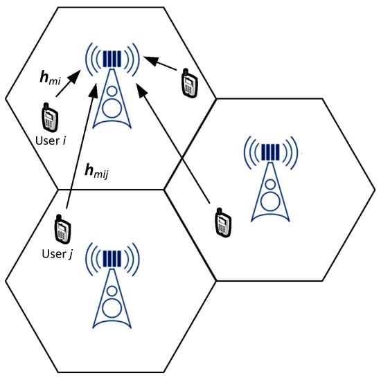
Figure 1.
Illustration of the considered system modeling drawn on the uplink data transmissions of a multi-cell interference network consisting of multiple base stations and mobile users.
Problem (3) is a type of sum-of-ratios problem with non-deterministic polynomial-time hardness (NP-hard) in its computational complexity, meaning that it belongs to the hardest class of problems to resolve explicitly and integrate in practice. Traditionally, such complexities are tracked by transforming problems such as (3) into simpler forms, using variable relaxation methods [,], which, on the other hand, introduce considerable truncation errors that compromise the convergence and accuracy of their solutions. To bypass such issues, the recent studies of [,,,] approach NP-hard types of problems with ANN modeling to obtain their solutions by using the trained neural network. For the sake of clarity, in the following Section 3, we build such an ANN model by elaborating on the parameters of the considered WSEE system modeling.
3. Artificial Neural Network Architecture for the Energy Efficiency Problem
The aim is to resolve problem (3) by deriving the power allocations as closed-form functions of the propagation channels , and the power threshold parameters so that the computation of the optimal power allocation can have negligible complexity, i.e., to track the fading channel variations and update in real time. To do so, we compact the nominator and denominator of the data rate expression in (1) by defining the channel realization vectors with , , and re-structure the WSEE problem (3) using the map as follows:
where is the vector with elements of the optimal power allocation coefficients of the L users corresponding to the M BS indexing, and is the set of real numbers. At this point, we recall the ANN universal approximation property, which yields the input–output relationship of a feed-forward neural network with fully-connected layers, capable of emulating any continuous function []. Indeed, as , the WSEE function in (2) is continuous, which facilitates approximating the map in (4) with an ANN model of fully-connected feed-forward layers, i.e., an input layer based on the realization of the parameter vector and an output layer based on the power allocation vector that, in essence, stands as an estimate of the optimal power allocation vector corresponding to input . Note that due to feed-forward, not only are these two input–output layers created, but also K additional “hidden” neural layers are generated as well. To enumerate all the neural layers, we label the input layer as layer-0, the first “hidden” layer as layer-1 with neurons, the k-th “hidden” layer as layer-k with neurons, and so on, until the output layer-, which includes neurons, as illustrated in Figure 2. In such a fully-connected ANN system, each layer has neurons in total, with each neuron n computing the following:
where (i) represents the output vector of layer k, (ii) the neuron-dependent weights, (iii) the neuron-dependent bias terms, and (iv) is the activation function of neuron n in layer-k. From (5), we see that although each neuron can perform simple operations, by combining the processing of multiple neurons in a single ANN, the system can perform complex tasks and obtain the overall input–output map in (4), which can approximate virtually any type of optimization function. The challenge, however, is how to configure the weights and bias terms for achieving the desired approximation accuracy. This can be resolved by training the considered ANN system using a supervised procedure, where a certain training set of optimal power allocations can be deployed as the collection of channel realizations and the corresponding optimal power allocations of training tuples . In other words, the training set contains examples of desired power allocation vectors corresponding to some possible configurations of system parameters , whereas, by exploiting these examples, the system can learn to predict the power allocation for new realizations of that are not included in the running training set. More specifically, by setting , the error measure between the actual and desired outputs in (5), the ANN training problem can be written as follows:
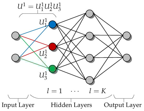
Figure 2.
Illustration of the channel transition between two layers during the ANN training process. To attain a stable state (i.e., the optimal result) the ANN needs access to multiple layers (i.e., input/output/hidden layers) at any given time.
Problem (6) can be straightforwardly resolved by the recently-announced techniques based on the stochastic gradient descent (SGD) method [,,,]. That is, for generating the training set in (6), the generic WSEE maximization problem (3) should be reformulated by means of normalizing its maximum transmit power coefficients , which requires transforming the variable into for all for constraining these power coefficients to lie within the closed interval . Using the variable transformation , the WSEE expression in (2) becomes and the generic WSEE problem (3) can be rewritten into its equivalent form (i.e., suitable for applying SGD) as follows:
where , , for all . In problem (7), the normalized ANN training set is with the parameter vector to be able to be conveniently resolved, using the improved branch-and-bound method proposed in []. Note that the importance in reformulating the initial problem (3) into (7) is that for any value of the maximum power vectors , the obtained optimal solution ensures that the transmit powers are lying within [0, 1]. Consequently, problem (7) will have much weaker dependency between the optimal solution and the maximum power constraints, compared to the problem (3). Besides this, problem (7) gives a simpler structure of the optimal solution as a function of the input parameters , among which we find the maximum power constraints , which simplifies the task of learning the optimal power allocation rule.
After the training phase, the resulting ANN input–output relationship provides an approximation of the optimal power allocation policy, which can be written in closed-form by considering the composition of the affine combinations and activation functions of all neurons. As shown in [,], such an approach provides accurate results with limited complexity, which makes NP-hard problem optimization (such as ANN-driven WSEE optimization) able to be applied in close-to-real-time, i.e., far faster and reliably than conventional relaxations discussed previously in Section 2.
4. Deep Quantum Neural Network Architecture for the Energy Efficiency Problem
By exploiting the quantum advantage [], it is anticipated that QNN will be able to solve the WSEE optimization problem (3) with comparable or better efficacy than its classical ANN counterpart. This is because upon realizing the ANN training process as a variational quantum circuit built on a continuous variable architecture, the training process can be enabled to encode quantum information in continuous degrees of freedom, i.e., by exploiting the amplitudes of the propagation channels and . That means that the feed-forward neural network can switch its building blocks from classical to quantum neurons, which, in turn, enterprise the computations of the power allocations by considering not only the system parameters of their own k layer, but all the layers. Such a feature is known as universal quantum computation [] and enables fast optimization with minimum memory demands because the number of the required qubits depends only on the width of the network at hand.
In this respect, we model the QNN training as a quantum circuit of multiple quantum perceptrons, where each perceptron is deemed to be a general unitary operator acting on m input qubits and n output qubits. That means that each perceptron can (i) be built using L hidden layers of qubits, (ii) act on an initial input state of qubits, and (iii) produce an output state of qubits that can be represented by the following:
where is the QNN quantum circuit and is the layer-specific perceptron expressed as the unitary operator of the product of the qubits between adjusting layers, e.g., perceptron reflects to the qubits between layer- and layer-l, with . Note that, as perceptrons are arbitrary unitary operators, they may not commute within the QNN, e.g., as shown in Figure 3, meaning that the order of their operations can be defined as the composition of a sequence of completely positive layer-to-layer transition maps, i.e., the following:
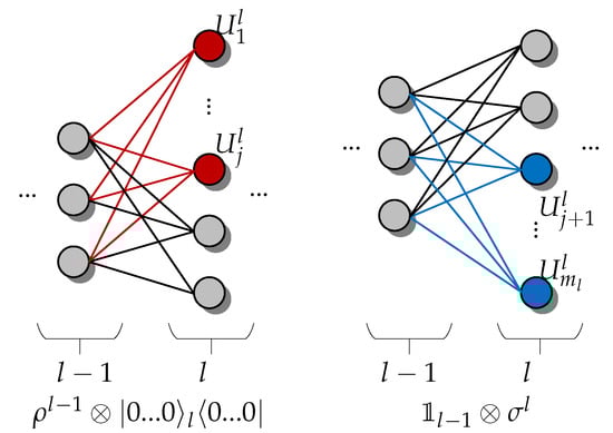
Figure 3.
Illustration of the channel transition between two layers during the QNN training process. To attain a stable state (i.e., the optimal result) the QNN needs to only access two layers at any given time, which greatly reduces the memory requirements compared to ANNs, which require access to more than two (multiple) layers each time (recall Figure 2 for example).
For example, in (9) is the j-th perceptron acting on previous layers and the current layer l, while is the total number of perceptrons acting on layers and l. On this basis, the QNN mapping in (9) facilitates the information data to propagate from the input to the output, which naturally works as a feed-forward neural network; thus, it corresponds to the classical ANN mapping in (4) of the generic WSEE problem (3). More importantly, adopting the mapping in (9), the QNN training can be performed with similar algorithmic logic as that of the classical ANN system based on the mapping in (4), i.e., by following a quantum analogue of the so-called back-propagation algorithm []. Recall that back-propagation aims at facilitating the training phase to obtain the output density matrix as closer to the desired output , which corresponds to the input . As such, we integrate back-propagation of (9) by setting the training function as follows:
which is known in the field of quantum information theory as the fidelity function []. Particularly, function C in (10) helps to (i) estimate the perceptrons as quantum states averaged over the training data, and (ii) quantify the difference between the output and a certain (desired) output by varying between 0 (worst estimation) and 1 (best estimation). For example, C can be minimized by updating the perceptrons unitary operators in the QNN training (9), i.e., , where is the matrix with all system parameters of the corresponding perceptron unitary operator and , the step size of the SGD algorithm. In view of (10), we can define the QNN learning rate and the update matrices for each perceptron j at layer l as follows:
and is the join channel to , which is the transition channel from layer to layer l, e.g., as illustrated in Figure 3.
Relying on (10), (11) and the feed-forward rationale of the SGD algorithm, we present in Algorithm 1 the pseudo-code to structurize the QNN deep-learning that derives the optimal power allocations of the WSEE problem (3). Notice the key contribution of Algorithm 1 that computes the trace over all qubits (i.e., in line 9) independently from , which gives rise to two important features for QNN operation. First, recalling that one of the merits of SGD rationale is that the parameter matrices K can be computed layer-by-layer without any need to rely on additional unitary operators of the full quantum system [], Algorithm 1 has a smaller step size than the ANN training in (6), which speeds up QNN convergence toward deriving the optimal WSEE power allocations. Second, by coordinating (10) with SGD, the computation of (9) at each step of Algorithm 1 involves only two layers, meaning that the size of the K matrices in the calculation of (10) depends only on the width of the network, rather than the width of each layer as required by the respective ANN training function in (5). This latter feature results in considerable memory savings and makes the proposed QNN deep-learning process highly practicable to apply in a realistic system setting and scaling. To demonstrate the practicability of our new QNN approach, the following Section 5 evaluates Algorithm 1 using benchmarks and simulations.
| Algorithm 1: Pseudo-code of the proposed quantum deep-learning process. |
| 1 Initialization:
2 Initialize Unitary randomly 3 Feed-forward: 4 For each batch of (,),, 5 (i) Apply the channel to the output state of layer 6 (ii) Tensor with layer l in state and apply : 7 (iii) Trace out layer and store 8 Update Network: 9 (i) Compute the parameter matrices 10 (ii) Update each unitary in which 11 Repeat: 12 Go to step-3 until the training function reaches its maximum. |
5. Numerical Evaluations
Before evaluating our findings, we recall that it is practicably impossible to simulate deep QNN learning algorithms using classical computers for more than a handful of qubits, due to the exponential growth of Hilbert space [,,]. Therefore, our evaluations will follow similar rationalism with the evaluations of the relevant studies in [,,,,], where the QNN performance is examined over a series of benchmarks to evaluate the size and number of the QNN training steps, e.g., if the algorithms can attain a stable state (i.e., derive the optimal result) in fast time (i.e., in as few as possible and short training steps).
We also recall that a striking feature of Algorithm 1 is that the parameter matrices can be calculated layer-by-layer without ever having to apply the unitary corresponding to the full quantum circuit on all the constituent qubits of the QNN in one go. In other words, we need only to access two layers at any given time (as shown in Figure 3), which greatly reduces the memory requirements of Algorithm 1 compared to ANNs, where access to more than two layers are required (as shown in Figure 2) with the respective increase in memory requirements. Hence, the size of the matrices in our calculation only scale with the width of the network, enabling us to train deep QNNs in a considerably less resource-costly and faster way than ANNs.
As such, to simulate the QNN deep-learning process in (11) toward optimizing the WSEE power allocation problem (3), we use a classical desktop computer with typical processing capacity (i.e., Intel i7 with 16 GB of RAM), which, in principle, is not designed to handle more than a handful of qubits (as stated previously). That means that, with mainstream equipment, we can execute Algorithm 1 for a four-layer QNN system of 16 neurons in total (i.e., 4 neurons for the input layer, 8 neurons for the two hidden layers and 4 neurons for the output layer), while the addition of more neurons is subject to future quantum-based equipment. Yet, even under conventional equipment, we demonstrate that such a four-layer QNN system can attain much higher performance than ANN systems of a bigger size, i.e., consisting of seven layers and 28 neurons in total. In addition, for fair simulation comparisons, we deliberate over a realistic system setting similar to [], which provides a generic Matlab coding of the so-called globally optimal energy efficient power control framework in interference networks.
On this basis, we translate the codes provided by [] (available online at []) to Python coding for producing a training module composed of 102,000 training samples for −30,…,−20 dB in 1 dB step and 10,200 validation samples, i.e., 10% of the overall training samples. In the produced training module, we split the total number of iterations into R rounds so that the parameter matrices in (11) can be re-initialized at the beginning of each feed-forward round of execution. Such matrix re-initialization ensures that the QNN training function C in (10) can increase with a smaller step size (i.e., more rapidly) than the ANN training function in (6) because each matrix includes all the necessary unitary operators of the full quantum system, rather than additional unitary operators corresponding to each perceptron as done in ANN. Having defined the rationale of our system setting, we proceed by updating the perceptron unitary, using and performing a random re-initialization and reshuffling with each batch size of 128 samples of data. We arrange [5,4,3,2] neurons over the considered four-layer QNN architecture, which consequences to 5 input perceptrons with 32 states and 2 output perceptrons with 4 states. In addition, we arrange the original information data over 17 sets of input data, and set zeros for the rest of the input state so that there is no need to add offset data for the output perceptrons, as the original output set is exactly equal to 4. Notice that this evaluation architecture is equivalent to the four-layer classical training process architecture with [32,16,8,4] neurons, which, without loss of generality, converges in iterations.
In Figure 4 we investigate the role of the parameter matrices in the QNN training process. Particularly, we set , learning rate , step size and 100 iterations to study the effect of on the value of the training function when it is initialized once and multiple times per step. We observe that when is initialized, Algorithm 1 can always produce lower cost values than those with 5 re-initializations across the number of batches, either for the first epoch or the fifth epoch. We also observe that by initializing multiple matrices , Algorithm 1 can attain its maximum cost value much faster than by initializing a single matrix for the whole training session. As result, the training function converges toward a steady state (optimal power allocation result) after 300 batches of data for multiple re-initializations.
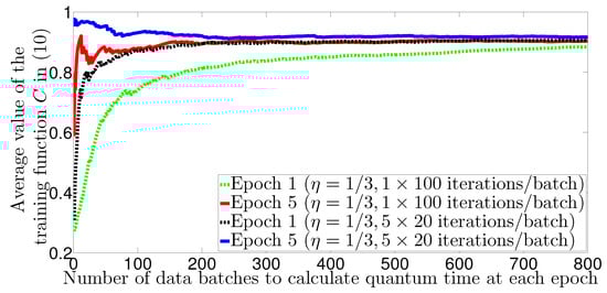
Figure 4.
Average value of the training function versus the number of data batches to calculate the quantum time for each epoch. We show that the proposed training function in (10) can indeed converge toward a steady state (optimal power allocation result) after 300 batches of data re-initializations.
In Figure 5, we examine the impact of the learning rate for the wireless communications data set. From the figure we see that the learning rate is too small to get stable unitary matrices compared to after 3 training epochs. We also see that by re-initializing multiple K matrices for 50 and 100 iterations within the training module, we can attain stable results (i.e., the WSEE optimal powers) after 3 epochs only (considerably fast). However, we notice that with a smaller learning rate, there are chances to attain higher cost value at the expense of increasing the epoch time, which may consume a longer total training time.
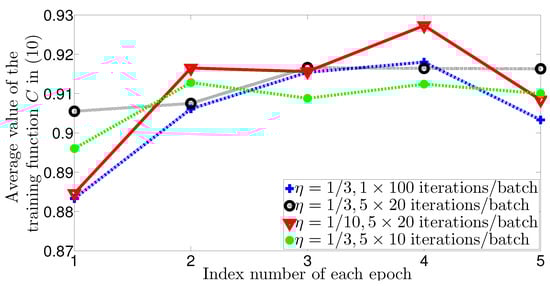
Figure 5.
Average value of the training function versus the index number of each epoch. We show that Algorithm 1 can reach the stable results (i.e., the WSEE optimal powers) considerably fast (after 3 epochs only). We also show that Algorithm 1 becomes more accurate by increasing the learning rate from to , which is expected and matches with the relevant algorithms’ behavior in [,,,,].
In Figure 6, we extend the globally optimal power control framework of [] by adding a training perceptron unitary operator to test the reliability of the proposed QNN architecture. For this experiment, we use 10,200 samples of new data for validation to observe that the trained perceptron unitary operator with learning rate of either or can provide better and more stable cost values after 4 epochs. We also notice from Figure 6 that the learning rate is too small for Algorithm 1 to reach a stable state in a short time, which matches with our previous observations in Figure 5 and implies that there is an optimal value of to be chosen during the training process so that Algorithm 1 can reach its actual minimum time of convergence. Nevertheless, even with small , the results of Figure 6 show that the training cost value and the validation cost value are almost comparable, which confirms the reliability of the proposed QNN architecture.
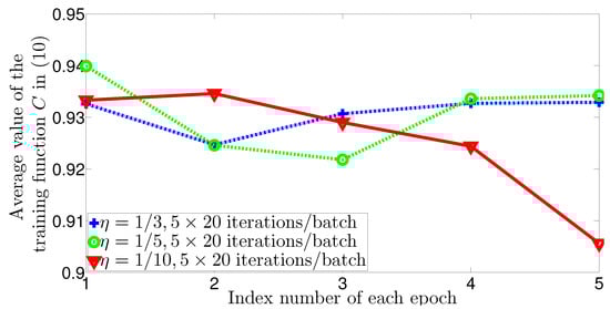
Figure 6.
Average value of the training function versus the index number of each epoch, using the training perceptron unitary operator. We show that besides optimizing the WSEE problem, Algorithm 1 can be also generalized to optimize the power control problem in []—although the two problems differ radically, Algorithm 1 can resolve both of them reliably and robustly, i.e., by requiring a similar training step size of and comparable implementation time between 3 and 4 epochs.
In Figure 7, Figure 8 and Figure 9, we examine the optimization accuracy and implementation time of the proposed QNN model in (8)–(11) in comparison to the ANN model in (4)–(7). For these experiments, we generated a training set from 2000 independent and identically distributed (i.i.d.) realizations of users’ positions and propagation channels. We considered each user to be randomly placed in the service area and that each user i is associated to the BS m with the strongest effective channel . For each channel realization, we apply Algorithm 1 to solve the WSEE problem (3) for dB in 1 dB step, which yields a training set of 102,000 samples. Note that for the comparison between QNN and ANN, besides the training set, we also need to define a validation set, which is commonly used during training to estimate the generalization performance of the QNN, i.e., the performance on a data set that the QNN was not trained on [].
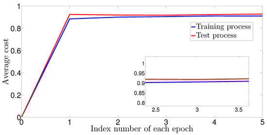
Figure 7.
Average cost versus the number of batches. The average cost measures the quantum fidelity, e.g., the QNN output and the desired output (the closed is better). We show that the training and validation sets quickly approach each other with a very small value of the same order of magnitude, e.g., in 3 epochs.
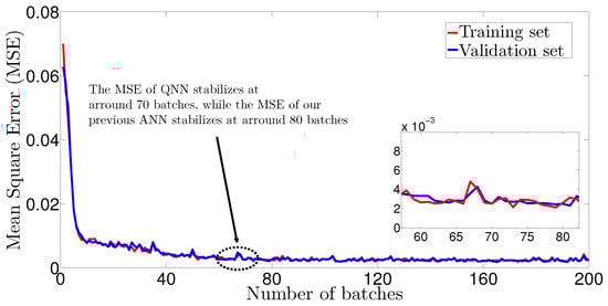
Figure 8.
Mean square error versus the number of epochs. We show that by feeding 800 batches of training data, our QNN model requires 70 epochs to stabilize its MSE—we recall that by using the same training set of 800 batches, our ANN model in [] requires 70 epochs to stabilize its MSE. Consequently, the performance of the QNN model in comparable with the performance of the ANN model for resolving the WSEE problem (3).
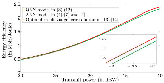
Figure 9.
Energy efficiency versus transmit power. We show that the QNN model in (8)–(11) derives similar energy efficiency results to the ANN model in (4)–(7) and [], while both QNN and ANN training models deviate at approximately 0.05 MBit/Joule, on average, from the actual optimal WSEE solution given in [,].
Having defined these training and validation sets, we plot in Figure 7 the average cost versus the number of epochs and in Figure 8 the mean square error (MSE) versus the number of epochs needed for WSEE optimization. From Figure 7, we observe that both the errors of the training and validation sets quickly approach a very small value of the same order of magnitude (in about 3 epochs), and that neither of the losses increases over time, which leads to the conclusion that the adopted training procedure fits the training data well, without underfitting or overfitting. Furthermore, we feed our QNN with 800 batches of training data to observe in Figure 8 that it needs approximately 70 epochs to stabilize its MSE (i.e., to reach the optimal WSEE result)—instead, in our previous study ([], Figure 2, p. 10), we feed with 800 batches of training data a classical ANN model to show that it can resolve the WSEE problem in 80 epochs. These results confirm that, given the same training data, the implementation speed of our QNN model is comparable and slightly faster than the implementation speed of the classical ANN model to resolve the same WSEE problem with similar optimization accuracy.
Finally, Figure 9 illustrates a comparison regarding the accuracy and actual optimization result between our QNN model and our classical ANN model []. Particularly, in Figure 9, we plot the energy efficiency (in bit/Joule) versus the transmitted power (in dBW) by following the setting mentioned previously and by taking as the evaluation metric the generic WSEE optimization method introduced in [,]. We observe that within the region of dBW, both QNN and ANN derive almost the same results as the actual optimal solution method in [,], while for the power region dBW, both the QNN and ANN training models deviate by approximately 0.05 Mbit/Joule on average from the actual WSEE solution. Nevertheless, the main point is that our QNN is proved to be as accurate as the ANN model. Therefore, by recalling our previous findings in Figure 7 and Figure 8, where we show that our feedforward QNN has slightly better trainability than its ANN analogue, we can conclude that there is potential for QNNs to perform faster training when applied on similar to WSEE problems, without showcasing overfit or underfit issues and by using classical computer hardware.
6. Conclusions
This paper studied the perspective of adapting quantum learning and training logic in wireless communication networks by proposing a new quantum neural network architecture for resolving the power control in energy efficiency optimization problems. We formulated the generic energy efficiency problem and approached it, using both classical and quantum neural network models. We conducted the design of the learning and training analysis for both these models to clarify their rationalism, with architectural differences and similarities. Furthermore, we proposed Algorithm 1 as the tangible mean of applying our QNN model, and conducted a series of benchmarks to evaluate its size and the number of training steps. We performed simulations to show that our algorithm can attain a stable state (i.e., derive the optimal result) in fast time (i.e., short training step), and that it can be generalized to other, more complicated problems, such as the power control problem in [], with comparable implementation time and accuracy. We also showed through simulations that our QNN model can attain the same accuracy with its ANN analogue by featuring slightly faster trainability for this specific energy efficiency problem. Based on these results, we believe that the perspective of quantum-oriented learning and training can play a significant role in the next-generation communications era in terms of decentralizing intelligence and saving computing and memory resources. The fact that our QNN model can run using classical computer hardware in a comparable manner to its ANN analogue model provides the incentive for future studies to clarify further links between quantum and communications engineering and improve QNNs to address other communications problems.
Author Contributions
Conceptualization, S.F.C.; methodology, S.F.C.; software, S.F.C. and H.S.L.; validation, M.A.K., Q.N. and A.Z.; formal analysis, S.F.C., H.S.L. and C.C.Z.; investigation, S.F.C., H.S.L. and C.C.Z.; resources, M.A.K., Q.N. and A.Z.; data curation, S.F.C. and H.S.L.; writing—original draft preparation, S.F.C. and C.C.Z.; writing—review and editing, C.C.Z., H.S.L. and S.F.C.; visualization, S.F.C., H.S.L. and C.C.Z.; All authors have read and agreed to the published version of the manuscript.
Funding
This research received no external funding.
Data Availability Statement
Not applicable.
Acknowledgments
The authors would like to thank Robert Salzmann at the Center for Quantum Information and Foundations, University of Cambridge, for his technical assistance.
Conflicts of Interest
The authors declare no conflict of interest.
References
- Zappone, A.; Renzo, M.D.; Debbah, M. Wireless networks design in the era of deep learning: Model-based, AI-based, or both? IEEE Trans. Commun. 2019, 67, 7331–7376. [Google Scholar] [CrossRef] [Green Version]
- Zappone, A.; Renzo, M.D.; Debbah, M.; Lam, T.T.; Qian, X. Model-aided wireless artificial intelligence: Embedding expert knowledge in deep neural networks towards wireless systems optimization. IEEE Vehic. Technol. Mag. 2019, 14, 60–69. [Google Scholar] [CrossRef]
- Aïmeur, E.; Brassard, G.; Gambs, S. Machine Learning in a Quantum World. In Advances in Artificial Intelligence; Lamontagne, L., Marchand, M., Eds.; Lecture Notes in Computer Science; Springer: Berlin/Heidelberg, Germany, 2006; Volume 4013. [Google Scholar]
- Marquardt, F. Machine learning and quantum devices. SciPost Phys. Lect. Notes 2021, 29, 21. [Google Scholar]
- Tiersch, M.; Ganahl, E.J.; Briegel, H.J. Adaptive quantum computation in changing environments using projective simulation. Sci. Rep. 2015, 5, 12874. [Google Scholar] [CrossRef] [PubMed] [Green Version]
- Lovett, N.B.; Crosnier, C.; Perarnau-Llobet, M.; Sanders, B.C. Differential evolution for many-particle adaptive quantum metrology. Phys. Rev. Lett. 2013, 110, 220501. [Google Scholar] [CrossRef] [PubMed] [Green Version]
- Banchi, L.; Grant, E.; Rocchetto, A.; Severini, S. Modelling non-Markovian quantum processes with recurrent neural networks. New J. Phys. 2018, 20, 123030. [Google Scholar] [CrossRef]
- Porotti, R.; Tamascelli, D.; Restelli, M. Coherent transport of quantum states by deep reinforcement learning. Commun. Phys. 2019, 2, 61. [Google Scholar] [CrossRef] [Green Version]
- Aïmeur, E.; Brassard, G.; Gambs, S. Quantum speed-up for unsupervised learning. Mach. Learn. 2013, 90, 261. [Google Scholar] [CrossRef] [Green Version]
- Paparo, G.D.; Dunjko, V.; Makmal, A.; Martin-Delgado, M.A.; Briegel, H.J. Quantum speedup for active learning agents. Phys. Rev. X 2014, 4, 031002. [Google Scholar] [CrossRef]
- Amin, M.H.; Andriyash, E.; Rolfe, J.; Kulchytskyy, B.; Melko, R. Quantum Boltzmann machine. Phys. Rev. X 2018, 8, 021050. [Google Scholar] [CrossRef] [Green Version]
- Sentís, G.; Monràs, A.; Muñoz-Tapia, R.; Calsamiglia, J.; Bagan, E. Unsupervised classification of quantum data. Phys. Rev. X 2019, 9, 041029. [Google Scholar] [CrossRef] [Green Version]
- Allcock, J.; Hsieh, C.; Kerenidis, I.; Zhang, S. Quantum Algorithms for Feed-Forward Neural Networks. arXiv 2019, arXiv:1812.03089. [Google Scholar]
- Beer, K.; Boundarenko, D.; Farrelly, T.; Osbotne, T.J.; Salzmann, R.; Wolf, R. Efficient Learning for Deep Quantum Neural Networks. arXiv 2019, arXiv:1902.10445. [Google Scholar]
- Gyongyosi, L.; Imre, S. Training Optimization for Gate-Model Quantum Neural Networks. J. Nat. Res. 2019, 9, 12679. [Google Scholar] [CrossRef] [Green Version]
- Choudhury, S.; Dutta, A.; Ray, D. Chaos and Complexity from Quantum Neural Network: A study with Diffusion Metric in Machine Learning. arXiv 2021, arXiv:2011.07145. [Google Scholar]
- Bhattacharyya, A.; Chemissany, W.; Haque, S.S.; Murugan, J.; Yan, B. The Multi-faceted Inverted Harmonic Oscillator: Chaos and Complexity. arXiv 2021, arXiv:2007.01232. [Google Scholar]
- Lloyd, S.; Mohseni, M.; Rebentrost, P. Quantum algorithms for supervised and unsupervised machine learning. arXiv 2013, arXiv:1307.0411. [Google Scholar]
- Abbas, A.; Sutter, D.; Zoufal, C.; Lucchi, A.; Figalli, A.; Woerner, S. The power of quantum neural networks. arXiv 2020, arXiv:2011.00027. [Google Scholar]
- Zhang, Y.; Ni, Q. Recent Advances in Quantum Machine Learning. Wiley J. Quantum Eng. 2020, 2, 1–20. [Google Scholar] [CrossRef] [Green Version]
- Matthiesen, B.; Zappone, A.; Besser, K.L.; Jorswieck, E.A.; Debbah, M. A Globally Optimal Energy-Efficient Power Control Framework and its Efficient Implementation in Wireless Interference Networks. IEEE Trans. Signal Process. 2020, 68, 3887–3902. [Google Scholar] [CrossRef]
- Lee, W.; Kim, M.; Cho, D. Deep Power Control: Transmit Power Control Scheme Based on Convolutional Neural Network. IEEE Commun. Lett. 2018, 22, 1276–1279. [Google Scholar] [CrossRef]
- Zarakovitis, C.C.; Ni, Q.; Spiliotis, J. New Energy Efficiency Metric With Imperfect Channel Considerations for OFDMA Systems. IEEE Wirel. Commun. Lett. 2014, 3, 473–476. [Google Scholar] [CrossRef]
- Zarakovitis, C.C.; Ni, Q.; Spiliotis, J. Energy-Efficient Green Wireless Communication Systems with Imperfect CSI and Data Outage. IEEE J. Sel. Areas Commun. 2016, 34, 3108–3126. [Google Scholar] [CrossRef] [Green Version]
- Leshno, M.; Lin, V.Y.; Schocken, S. Multilayer Feed-Forward Networks with a Non-polynomial Activation Function can Approximate any Function. Neural Netw. 1993, 6, 861–867. [Google Scholar] [CrossRef] [Green Version]
- Beer, K.; Bondarenko, D.; Farrelly, T. Training deep quantum neural networks. Nat. Commun. 2020, 11, 808. [Google Scholar] [CrossRef] [Green Version]
- Nielsen, M.A.; Chuang, I.L. Quantum Computation and Quantum Information; Cambridge Univ. Press: Cambridge, UK, 2010. [Google Scholar]
- Generic Matlab Coding for Simulating Quantum Deep Learning Processes. Available online: https://github.com/R8monaW/DeepQNN (accessed on 23 February 2021).
Short Biography of Authors
 | Chien Su Fong is a principal researcher at MIMOS Berhad. He received the B.Sc. and M.Sc. degrees from the University of Malaya, Malaysia, in 1995 and 1998, respectively, and the Ph.D. degree from Multimedia University, Malaysia, in 2002. He has been serving as a TPC member or a reviewer for ICACCI, ICP, SETCAC, ISCIT, GNDS, Ad Hoc Networks, and CNCT. He has published several of tens of conference and refereed journal papers and holds few patents. His current research interests include green communications, optimization, applications of bio-inspired algorithm, machine learning, neural networks, and quantum computing algorithms. He is one of the editors-in-chief of Bio-Inspired Computation in Telecommunications. |
 | Heng Siong Lim received the BEng (Hons) degree in electrical engineering from Universiti Teknologi Malaysia in 1999, and the MEngSc and PhD degrees from Multimedia University in 2002 and 2008, respectively, where he is currently an Associate Professor with the Faculty of Engineering and Technology. His research interests include signal processing and receiver design for wireless communications. |
 | Michail Alexandros Kourtis received his PhD from the University of the Basque Country (UPV/EHU) in 2018 and from 2012 is a Research Associate at NCSR “Demokritos” working on various H2020 research projects. His research interests include Network Function Virtualization, 5G and Network Slicing. |
 | Qiang Ni received the B.Sc., M.Sc., and Ph.D. degrees from the Huazhong University of Science and Technology (HUST), China, all in engineering. He is currently a Professor and the Head of the Communication Systems Group with InfoLab21, School of Computing and Communications, Lancaster University, Lancaster, U.K. He has published over 150 papers. His main research interests lie in the area of future generation communications and networking, including green communications and networking, cognitive radios, heterogeneous networks, 5G, energy harvesting, IoT, and vehicular networks. He was an IEEE 802.11 Wireless Standard Working Group Voting Member and a Contributor to the IEEE Wireless Standards. |
 | Alessio Zappone obtained his Ph.D. degree in electrical engineering in 2011 from the University of Cassino and Southern Lazio, Cassino, Italy. Afterwards, he has been with TU Dresden, Germany, from 2012 to 2016. From 2017 to 2019 he was the recipient of an Individual Marie Curie fellowship for experienced researchers, carried out at CentraleSupelec, Paris, France. He is now a tenured professor at the university of Cassino and Southern Lazio, Italy. He is an IEEE senior member, serves as senior area editor for the IEEE Signal Processing Letters, and served twice as guest editor for the IEEE Journal on Selected Areas on Communications. He chairs the RIS special interest group REFLECTIONS, activated within the Signal Processing for Computing and Communications Technical Committee. |
 | Charilaos C. Zarakovitis received the BSc degree from the Technical University of Crete, Greece, in 2003, the M.Sc and G.C.Eng degrees from the Dublin Institute of Technology, Ireland, in 2004 and 2005, and the M.Phil and Ph.D degrees from Brunel University, London, UK, in 2006 and 2012, respectively, all in electronic engineering. In Academia, he has worked as Senior Researcher at (i) Infolab21, Lancaster University UK, (ii) 5GIC, University of Surrey UK, and (iii) MNLab, National Centre for Scientific Research “DEMOKRITOS” Greece. In Industry, he has worked as Chief R&D Engineer at AXON LOGIC Greece, and as R&D Engineer at MOTOROLA UK, INTRACOM S.A Greece, and NOKIA-SIEMENS-NETWORKS UK. His research interests include Deep Learning, Quantum Neural Networks, green communications, bioinspired and game-theoretic decision-making systems, network optimization, cognitive radios, Ad-Hoc Clouds, among others. |
Publisher’s Note: MDPI stays neutral with regard to jurisdictional claims in published maps and institutional affiliations. |
© 2021 by the authors. Licensee MDPI, Basel, Switzerland. This article is an open access article distributed under the terms and conditions of the Creative Commons Attribution (CC BY) license (https://creativecommons.org/licenses/by/4.0/).