
A High Resolution Spatiotemporal Urban Heat Load Model for GB


UCL Energy Institute, London WC1H 0NN, UK
*
Author to whom correspondence should be addressed.
Energies 2021, 14(14), 4078; https://doi.org/10.3390/en14144078
Submission received: 31 May 2021
/
Revised: 29 June 2021
/
Accepted: 30 June 2021
/
Published: 6 July 2021
(This article belongs to the Special Issue Bottom-Up Urban Building Energy Modelling)
Abstract
:The decarbonisation of heating in the United Kingdom is likely to entail both the mass adoption of heat pumps and widespread development of district heating infrastructure. Estimation of the spatially disaggregated heat demand is needed for both electrical distribution network with electrified heating and for the development of district heating. The temporal variation of heat demand is important when considering the operation of district heating, thermal energy storage and electrical grid storage. The difference between the national and urban heat demands profiles will vary due to the type and occupancy of buildings leading to temporal variations which have not been widely surveyed. This paper develops a high-resolution spatiotemporal heat load model for Great Britain (GB: England, Scotland a Wales) by identifying the appropriate datasets, archetype segmentation and characterisation for the domestic and nondomestic building stock. This is applied to a thermal model and calibrated on the local scale using gas consumption statistics. The annual GB heat demand was in close agreement with other estimates and the peak demand was 219 GWth. The urban heat demand was found to have a lower peak to trough ratio than the average national demand profile. This will have important implications for the uptake of heating technologies and design of district heating.
1. Introduction
The Climate Change Act [1] sets a target for the United Kingdom (UK) to reduce greenhouse gas emissions by 80% from 1990 baseline levels. The government has since committed to a net-zero target for the electricity system [2]. The provision of heat and hot water for building accounts for around 40% of all energy consumption and 20% of greenhouse gas emissions in the UK. To meets these targets, emissions from the building sector are required to be near zero [3]. This is expected to drive the expansion of district heating (DH) to deliver low carbon space and water heating. The decarbonisation of electricity generation in the UK is facilitating a shift away from fossil-based heat generation to electrified heating with heat pumps [4]. Heat pumps are likely to play a key role in the decarbonisation of the heating sector and their integration into DH systems is a promising application [5,6]. Indeed, Part L of the building regulation now encourages developers to consider the use of heat pumps and connection to DH in order to not exceed target emission rates [7].
Hourly space heat and hot water demand estimates are required to determine the hourly electrified heat load of modelled electricity scenarios and for use in modelling of urban district heating networks. The temporal variation of energy demand is an important factor when considering the sizing and operation of energy storage, grid storage (in the case of the power system) and thermal storage in DH networks. It is likely that there will be differences in the daily load profile between the urban and non-urban areas due to the type of buildings and the occupancy of buildings and the use patterns leading to temporal variations, which are important factor but not widely surveyed. In addition, estimation of the locally disaggregated heat load is needed for both electrical distribution network with electrified heating and for the identification of potential areas for the development of DH. This paper develops a spatiotemporal heat load model—HeLoM, with requirements that can be summarised as:
- Capture the entire hourly space heat and hot water load based on historic meteorological data for Great Britain (GB)
- Disaggregate the urban load as a proxy for DH demand
Urban loads are split from the remainder because these are typically the areas with the highest heat demand density and therefore are the most appropriate areas to consider for district heating because network costs are generally lower per unit of heat load. The disaggregation of urban heat load can be achieved by having a spatially disaggregated hourly heat load with the highest heat demand per unit area being assumed as urban.
1.1. Literature Review of Heat Load Modelling
Most recent national heat demand studies have focused on domestic heating. Space and hot water heating accounts for 40% of energy demand in the UK with the domestic sector making up just over two-thirds of this [8,9].
Building stock energy simulations range from highly detailed simulations of individual buildings, up to the scale of the entire stock containing many built form types and uses. In building energy modelling, top-down models normally explore the inter-relationship of demand with key factors such as construction age or demography; this can be described as a deductive method [10]. Bottom-up models tend to disaggregate the components of energy demand into its various components, often employing a building physics-based approach [11]. At higher spatial resolutions, the impact of an individual building is greater and thus the need for accuracy increases. The bottom up approach is hence preferred by designers and planners. However, it can be difficult to calibrate and validate such models without large scale data collection, which can often be impractical on such a scale. For this reason, many building stock energy models use building archetypes as a representation of a statistically average form of a typology that can be multiplied to the national stock scale. Most building energy models aggregate energy demand from a large number of buildings and can provide estimates of energy use if the ratio of built form types is altered.
To highlight the growing importance of this field, there have been several reviews of building stock energy models conducted in recent years [10,11,12,13]. A notable example used for the UK is the BRE’s Domestic Energy Model (BREDEM) [14,15].
Reinhart and Davila [13] review the design of existing bottom-up building stock energy models. They describe the steps required to construct such models as:
- Data input and organization
- Thermal modelling
- Result validation
They identify the information that is required to generate building energy models. This includes regional weather data, building form, construction and operation data, and finally building occupancy or usage. To estimate future demand, inferences have to be made regarding the building stock and climate conditions. The authors state that the biggest challenge for such models is in the definition of the archetypes to recreate the simulated building stock.
In the review of Kavgic et al. [11], the authors compared eight different bottom-up energy stock models, including five UK based models. All the UK models derived their calculation from a version of the BREDEM. All the models reviewed output data at either an annual resolution or in two cases, a monthly resolution. They vary in the number of archetypes or dwelling types, ranging from just two age categories to over 8000 unique combinations of dwelling type including age, form, construction, and heating method. Of these, only the Community Domestic Energy Model [16] contained a spatial resolution higher than the national scale, but only for the existing stock, while most others were used for some scenario analysis.
Sousa et al. [10] comprehensively analysed 29 housing stock energy models. A common concern raised by both reviews is that the current approaches are limited in scope due to a lack of transparency, often being irreplicable and having no access to the core calculation modules. Much of this is due to the scale of the challenge, with some 25 million homes in the UK and a limited amount of cross-sectional surveys from which to base modelling assumption and data validation. There exists a large variation in their designs, both spatially and temporally [12]. None of the UK-based models have disaggregated urban loads from national at an hourly resolution. The reviews also note that improved data collection standards are needed as well as computational resources to capture detail at high spatial and temporal resolutions (as shown in Box 1).
Box 1. Output areas and geographic subdivisions
- Output areas (OA) have been used for data collection since the 2001 Census. They are the smallest geographical unit for which data is collected and designed to be largely homogenous. Small are statistics are reported at the Lower Super Output Area (LSOA), consisting of multiple adjacent OAs and Middle Super Output Area (MSOA), constructed from adjacent LSOAs. LSOAs are designed to have a population of 1000–3000 and MSOAs 5000–15,000.
- The Scottish equivalents of LSOA and MSOA are Data Zones (DZ) and Intermediate Zones (IZ). For convenience only the former terminology will be used. Scottish DZ are also smaller than LSOAs, each DZ contains approximately 500–1200 residents and IZs between 2500–6000.
- Another common subdivision used is the local authority (LA) which are governmental subdivisions. There are 397 LAs in GB of varied area and population.
1.1.1. National Demand
Prediction of peak demand with electrification is a key aim in many assessments of the national heat load. One of the few spatiotemporal studies has been conducted by Eggiman et al. [17]. They developed a high spatial and temporal resolution heat and electricity demand model to study the diffusion of heat pumps in the UK. The authors noted that the need to balance resolution with computing requirements and data availability is one of the main contributing factors towards the lack of spatiotemporal projections of UK heat demand. They use the LA subdivision and disaggregate between domestic, service, and industrial sectors. The temporal variation for electricity was calibrated via electricity transmission system data but similar data is not available for gas transmission, and therefore it was not validated. They use a heating degree day method to estimate heat demand and like most studies of this kind, they used a combination of yearly and daily load profiles to decompose annual energy use data into hourly temporal demand. A strength of this study is the use of technology specific load profile; they have differentiated between gas boiler demand profiles and heat pump profiles, notably using measured heat pump load profiles.
Another recent contribution towards national spatiotemporal heat demand modelling was conducted by Clegg and Mancarella [18]. They also use the LA level and heat demand was simulated for a single year in EnergyPlus using four domestic archetypes and four nondomestic archetypes to derive load profiles. These were mapped to the building stock with statistical variations in occupancy and in thermal performance characteristics to recreate demand diversity. It was found that regional half hourly peaks were 200% larger than the average daily demand. The authors use this to analyse the impact of the evolution of heating technologies on the gas and electricity network. A similar method using EnergyPlus generated profiles was applied at the postcode level and aggregated to city level demand [19].
Taylor et al. [20] created a high resolution (1 km square) spatial mapping of heat and electricity demand to study the diffusion of heat pumps. They used socio-economic census data combined with historic energy demand data. Assumptions were made to increase the spatial resolution of demand, but with a static analysis capturing only annual demand. Future demands were extrapolated factors from the base year.
Quiggin and Buswell [21] used historic weather data to analyse the impact of heat electrification. They combined a heating degree day with measured district heating demand to generate domestic load profiles and flat nondomestic load profiles. The authors concluded that peak electricity demand will be significant, and that demand side management can provide an important balancing function.
Other notable contributions in estimating national heat demand includes the work of Sansom [22] who used a regression analysis using historic weather and gas demand data to estimate national heat load. Daily heat demand was combined with measured load profiles to create half hourly demand profile for 2010.
It is estimated that there are over two million nondomestic buildings in the UK compared to over 24 million dwellings but comprises around a fifth of the space and water heat demand [4]. The studies that primarily focus on the domestic sector in the UK outnumber the studies in nondomestic modelling. Reasons for this include the well-established complexity of the nondomestic building stock [23,24,25,26].
1.1.2. Domestic Modelling
There are a several commonly used bottom up domestic energy models for the national housing stock [27]. Most are based on the English Housing Survey EHS (and prior to that the EHCS) which is an ongoing stratified random national survey covering the housing stock [28]. The segmentations used in the survey are commonly used in modelling assumptions. It provides the main input to the Cambridge Housing Model (CHM), a policy advice tool to estimate energy demand from the housing stock, and also provides the basis for other studies [29].
Cheng and Steemers [27] note that a common weakness of the current bottom up stock models is the use of generic occupant behaviour. Considering this, a large differentiating factor in their model—the Domestic Energy and Carbon Model (DECM), has been the use of multiple occupancy profiles based on employment status from socio-economic census data. DECM disaggregates output down to the LA level. The heat demand is estimated based on the SAP method from the BRE [30]; due to this, only yearly results are output from the model. They find that dwelling type and socio-economic factors account for 85% of the variation in consumption between LAs.
BREDEM is described as a methodology to calculate domestic building energy consumption for different end uses and is widely employed as the core of other domestic energy models due to its adaptability [11]. It uses heat balances and simple empirical relationships that can be expanded upon to estimate annual domestic energy consumption [31]. Examples that use BREDEM include the Community Domestic Energy Model (CDEM) [16]. CDEM combines archetypes with the BREDEM method to investigate efficiency interventions. Other models utilise GIS tools to infer built form and orientation to model the energy consumption using BREDEM at the neighbourhood scale [32]. The use of GIS based methods to analyse and gather data is becoming prevalent in building stock modelling. Oikonomou et al. [33] looked at the urban heart island effect for London and the risk of overheating in dwellings. They use GIS data of building form and orientation to conduct simulations in EnergyPlus. Occupancy profiles were based on the work of Yao and Steemers [34]. Another GIS based approach applied polygon information, LIDAR, and thermal imaging to the Cambridge Housing Model to produce energy demand profiles at the neighbourhood level [35]. There is potential to use this methodology on a wider scale by city planning but the large computing requirements when scaled to larger areas remains a key challenge [36].
In contrast to the bottom-up models presented, Watson et al. [37] use a top-down approach to determine a regression model using historical gas demand and weather data. This is combined with load profiles obtained from measured heat pump profiles and differentiated by mean outdoor temperature. The study modelled a high temporal resolution and the results can provide a useful comparison for national heat demand.
1.1.3. Nondomestic Modelling
The difficulties involved in modelling the nondomestic stock include the high degree of heterogeneity, both within and across use categories. Perhaps the biggest challenge involves the availability of quality data [20]. The energy end use is more varied, meaning measurements of gas consumption cannot be reliably used as a proxy for heating, the most comprehensive resource available being property taxation data collected by the Valuation Office Agency (VOA). However, this does not identify all floor area in nondomestic sites such as hospitals or libraries and omits certain use categories such as agricultural buildings or places of worship. A second important data source is Display Energy Certificates (DECs) for public access properties in England and Wales, but these can also be inaccurate for many of the same reasons [38]. In 2014 DECC commissioned the Building Energy Efficiency Survey (BEES) [39] to assess and understand how energy is used in the nondomestic stock across the different use categories. A comprehensive review of nondomestic stock modelling in the UK has been covered in Steadman et al. [40]. These have typically been in the form of a building database containing activity class and floor areas. The energy demand has then typically been estimated by simple steady state equations, such as energy intensities per floor area for a given activity class.
The CaRB2 model operates on this basic principle [41], using data from the above-mentioned sources, combined with a consumption data per activity type that was obtained from prior surveys. However, as it draws upon the VOA data, it only covers England and Wales. The Cambridge Nondomestic Energy Model (CNDM) has been developed with similar methods to the CHM [42]. This is achieved by segmenting disaggregating the nondomestic stock into different building archetypes and applying a steady state energy model. The disaggregation included built form, HVAC type, building age, location, and use which resulted in some 35,000 combinations. The CNDM also uses the taxation database disaggregated at a regional level with an annual breakdown of end use.
GIS approaches are also being used in nondomestic stock modelling, such as by Taylor et al. [43], who use ordnance survey data to create polygons of buildings for Leicester city centre. The 3DStock model is intended as a whole stock model but its treatment of the nondomestic stock merits attention [38]. It uses a GIS approach to combine a detailed representation of the urban building stock in select sub-city areas with taxation data, DECs, and energy consumption data. A key feature of 3DStock is that the model differentiates between buildings and premises for nondomestic sites. A single premise can be part of a building or multiple buildings, and the same building can have multiple premises. The energy consumption data (a database few other models have access to) for all modelled premises is then matched to the 3D representations of the buildings. It has so far only been applied to several sub-city areas and provides a high spatial resolution snapshot of energy consumption.
1.1.4. District Scale Modelling
There have been attempts at mapping the heat demand in the UK at a high spatial resolution such as the now defunct National Heat Map developed by the Centre for Sustainable Energy [44] for DECC which was designed with an emphasis on the location of heat networks and waste heat potential. Internationally, other such tools exist at the city scale, however these are only snapshots of heat demand intensity or annual consumption [45,46]. Tools such as CitySim [47] or Huber and Nytsch-Geusen [48] have been developed to aid urban planning and have been demonstrated with application to case studies, however these localised tools require extensive modelling data input. Numerous examples exist in the literature of localised studies to forecast heat load in district heating systems that use a variety of methods from detailed network simulation to statistical and machine learning methods [49,50,51,52,53]. As these are localised for specific districts and existing networks, these models can’t be applied directly to modelling districts in the UK without extensive data input and large assumptions. Methods of creating spatiotemporal energy demand for districts have been achieved by applying known spatial consumption to temporal profiles based on the distribution of building archetypes but the temporal profile can be difficult to validate particularly without comparative data at the same spatial resolution [54].
As already shown, GIS based methods to generate three-dimensional polygons are prevalent in the literature. Nouvel et al. [55] compared two methods: a thermal model applied to 3D reorientations and a statistical method using 2D GIS. They combined these methods to develop a framework to study heat loads at higher spatial resolutions using statistical method at the lower spatial resolution then applying a thermal model to 3D representations for higher spatial resolutions. Dogan and Reinhart [56] applied GIS to a mixed-use neighbourhood in Boston, USA. They generated 3D models that are then simulated in EnergyPlus to create hourly load profiles. Nageler et al. [57] applied a GIS to open source mapping data of an Austrian district to generate polygonal representations of buildings. Demand profiles were assigned to buildings using a thermal model and a database of archetypes. The authors of this study noted that computational resources were the main limiting factors on enlarging the modelled area.
1.1.5. Conclusion of Review
Building stock energy models in the UK are well established, particularly in the domestic sector. The segmentation of the building stock into archetypes is widely used, except in cases where a regression has been applied to historical data. The main data sources that are drawn upon are census data, historical consumption, and the EHS. Many studies and tools that map energy demand do so with a static state energy method or mapping historical annual consumption. Two recent studies have created a spatiotemporal analysis of energy demand [17,18]. The heat load modelling was achieved via either application of load profiles to heating degree day calculations or the generation of load profiles through building physics models with a reduced set of archetypes.
Achieving high accuracy is difficult due to the lack of data. Data on occupancy and when heating systems are operated is essential. This is one of the primary reasons that nondomestic modelling is harder than the well understood domestic sector. With (non-hourly metered) gas being the main heating vector in the UK, it has not been possible to use historical consumption alone to determine hourly loads, as is the case with electricity. With the increasing uptake in heat pumps however, this may be less of an issue in future. District heating load profiles are available and have been drawn upon in the literature to provide urban heat load profiles. However, the composition of the local building stock varies between locations. Existing high-resolution spatiotemporal models are not suitable for use or adaptation. Others that can be adapted are only national in scale, as is the case with the regression models.
2. Method
Each building is unique, not just in terms of the physical construction and location, but also in its occupancy and use. This model follows the approach of segmenting the stock into building archetypes. Once building archetypes are defined, a transient thermal simulation is developed to calculate the hourly heat demand using historical weather data. The advantages of using a custom a thermal model for simulating buildings is that it allows the efficacy of interventions such as altering insulation to be evaluated and enables the use of custom weather data to simulate heat demand. While individual building will be simulated, results will be stored at an aggregated level (LSOA or MSOA) and diversity is achieved by statistically varying occupancy.
A fundamental challenge in modelling the building stock is in the level of detail and attention afforded towards grouping similar constructions into segments or archetypes. The archetype approach is widely utilised in the framework bottom-up building stock modelling. A building stock can be represented by a sample of building archetypes that represent a statistical average for the archetype within the stock [58].
To develop archetypes, appropriate segmentations need to be identified prior to characterisation of thermal properties and occupancy. The most fundamental segmentation is differentiating between domestic and nondomestic. The archetype developed here will draw upon the work of a combination of previous studies. The open source datasets drawn upon for this work are shown in Table 1.
2.1. Domestic Archetype Segmentation
Most domestic archetypes used in modelling studies in the UK have extensively drawn on the English Housing Survey [65]. The EHS splits domestic buildings into seven archetypes: end and mid terrace, semi-detached, detached, bungalow, converted flat, and purpose built flat. The ONS data per LSOA reports on dwelling types as detached, semi-detached, terraced, purpose built flat, converted flat, and others such as bungalow or caravan. The ONS categories do not directly correspond to the EHS ones.
This model combines end terrace and mid terrace to correspond to the ONS reporting. While the ONS reports on purpose built and converted flats, converted flats have wide variety in form and the construction information in the available literature is largely for purpose-built flats. Therefore, all flat varieties will be treated as purpose-built flats. The same archetype segmentation has also been used in other studies [33,66]. The observed distribution of the used dwelling types is shown in Figure 1.
Each dwelling category is further split according to construction period. The VOA reports dwelling age in 12 build periods, from pre-1900 to post-2010, corresponding roughly to a decade in length while the EHS splits this into five build periods from pre-1919 to post-1990. The proportion of dwellings per age range has been applied to each dwelling type present in the LSOA. While it is likely that different dwelling types are built in different periods, the age variation per dwelling type is estimated from the overall distribution per LSOA as the data is provided per LSOA without further breakdown of age per dwelling type. This may be an issue with LSOA’s that have a diverse range of dwelling types and construction periods but in many smaller LSOA’s the construction type and age fall within a narrow range [67]. The distribution of dwelling build-period is shown in Figure 2.
The SAP assessment has 11 age bands that are often combined. Oikonomou et al. [33] use five age bands with multiple variations, reducing these to the 15 most commonly found in their modelled area. Mata et al. [58] combine six dwelling types with eight narrow and recent age bands, Cheng and Steemers [27] use ten age bands that become progressively narrower while Buttita et al. [69] use the EHS age bands but combine two of the periods. Table 2 summarises the archetypes used in other studies.
2.2. Domestic Archetype Characterisation
The form and fabric data for each archetype is used to estimate a specific heat loss (SHL) and thermal mass (ThM) from construction and fabric assumption per archetype. Dwelling archetype geometry will be taken directly from the English Housing Survey [70]. The specific heat loss will largely be derived from construction data from BREDEM 2012 [15] and glazing ratio and performance data are taken from the BRE’s SAP 2016 [71]. The thermal mass represents the heat capacity of a building or its ability to store heat. Construction and fabric play a large role in the thermal mass as do the internals of a dwelling. SAP gives thermal mass with a thermal mass parameter per unit floor area. It has three categories of light, medium, and heavy construction ranging from 100 to 450 kJ/m2K. The TMP used are adapted from Stamp [66] who provides estimates for the building archetypes used here and shows that older constructions tend to be heavier while newer constructions utilise modern lightweight construction methods and so have a lower TMP.
The power rating and efficiency of the heating system varies greatly between dwellings, and the power capacity determines to a large extent how it is operated. For the purposes of calibrating the heat load with gas consumption data, it is assumed that all buildings have a gas boiler with an average efficiency of 85% for heating and 75% for hot water [71,72]. The power ratings of the heating system per archetype are assumed from a conservative calculation of gas boiler power ratings using the domestic heating sizing method CE54 [73]. Table 3 summarises the data sources drawn upon for domestic archetype parameters and Table A1 in Appendix A contains all the estimates and parameters used for domestic archetype characterisation.
Domestic Occupancy
Mean occupancy has been adapted from the SAP methodology based on floor area [71]. Measured hourly gas consumption profiles have been used as a proxy for active occupancy profile and heating system operation for all dwelling archetypes. Average domestic heat load profiles in UK households exhibit a double peak pattern, with morning and evening peaks. From surveys on how dwellings are heated with various heating systems including gas boilers and heat pumps, it appears that dwellings are predominantly heating this way regardless of heating system and mixed work patterns [37,74,75]. Yao and Steemers [34] showed that the load profile is same across dwelling types, with the magnitude of peaks corresponding to the size of dwelling archetype. A normalised domestic load profile has been adapted from Wang et al. [76] to represent the probability of active occupancy and operation of heating as shown in Figure 3.
2.3. Nondomestic Archetype Segmentation
The nondomestic archetypes are based on the CaRB2 activity classifications which expand on the four VOA bulk classes: retail, office, industry, warehouse [38,59]. The primary source of data for nondomestic counts and floorspace as previously discussed is the VOA taxation database. The available data from CaRB2 contains activity classification and aggregated floor area per postcode which were combined to LSOA level by matching postcodes to output area without detail on activity type (due to data protection). While floor area has made available, this data is deemed inaccurate due to the method of taxation data collection where some classes (such as schools, hotels, and hospitals) do not have floor area records [77]. The CaRB2 activity classifications, count and floor areas are shown in Figure 4. For the purpose of urban load modelling, the five most important categories are office and shops (retail), followed by factories, warehouse, and hospitality. It was not possible to obtain localised Scottish nondomestic figures as the VOA database covers only England and Wales. Instead the overall count of each archetype in Scotland was scaled to each IZ using annual gas consumption data [63].
2.4. Nondomestic Archetype Characterisation
The occupancy and use of nondomestic buildings shows a large variation even within the same classification and there can be many different sizes and floor plans [78]. While classifications such as “offices” or “education” are generally occupied during normal working hours, the occupancy and usage can often vary with occupancy in the evenings and weekends.
The archetypes were adapted from analysis of the CaRB2 data by Barrett [79]. The mean floor areas for each category were calculated from the total gross internal area and archetype form was inferred from prior surveys of the nondomestic building stock [80,81,82]. A medium-weight construction TMP of 250 kJ/m2K was applied to all archetypes to derive a thermal mass. Benchmark guidelines were followed for the sizing of the heating system and determining internal heat gains in the various archetype activity classifications [83,84]. Where data and benchmarks for the archetype were not found, the figures were estimated from other archetypes.
Nondomestic internal gains are estimated from benchmark figures from CIBSE [84] Guide A. Offices and schools are well represented in other literature [85,86], but where the archetype data is unavailable, such as the case for industrial buildings, this has been estimated based on CIBSE Guide A. A summary of the nondomestic archetype parameters is shown in Table A2.
Nondomestic Occupancy
Building occupancy and use was determined mainly from analysis of hourly gas consumption data for 37 buildings provided by Sustainable Energy Limited [87]. Normalised profiles were extracted for each activity class available in the dataset as shown in Figure A2 and Figure A3. This was further supplemented through secondary studies on occupancy in offices, shops, health and educational buildings but for non-UK based buildings [88,89]. There are three categories where there is a lack of available data on occupancy: factory, warehouse, and transport. Factories and warehouses constitute 19% of the modelled stock and both are very diverse in their activity types. The factory classification can range from a food processing factory to newspaper print works while it is unclear to what extent warehouses are heated due the large floor area they occupy. Transport buildings are similarly diverse, from a train station to a petrol station. A 24-hour occupancy with higher daytime usage has been estimated for these categories as in shown in Figure A1.
2.5. Spatial Disaggregation
The highest level of spatial disaggregation is to the LSOA level. All GB domestic stock has been mapped to this spatial resolution. While the nondomestic activity classifications in the CaRB2 database were available per postcode in England and Wales, these were also mapped to the LSOA level. In Scotland, nondomestic stock counts were only available at the national aggregated scale, these were distributed per MSOA, weighted by MSOA nondomestic gas consumption.
Due to computing capacity and storage limitations, only selected MSOAs have been modelled. The gas demand per square kilometer has been estimated per MSOA using Standard Area Measurements, then ranked by gas consumption density. The top 20% cumulatively were chosen as representative of urban heat demand. A further 10% of largest absolute gas consumption were included to include a more representative consumption profile to scale to national level. The results for each LSOA and MSOA are stored in a table within an SQL database. Each hour or row of data contains roughly 1600 bytes of data. Six years of results for 10,226 individual LSOAs and MSOAs results in just over 40 GB of stored results.
Weather Data
Weather data is divided into GB regions (the highest tier of sub-national division). Weather stations were selected per region based on proximity to population centers and completeness of data, covering at least the period 2010–2016. The regional stations from which data is drawn upon is shown in Table 4.
Met office data was compiled ensuring that each station has been active since at least the beginning of 2010. Missing temperature (wet bulb) values were linearly interpolated unless large gaps of more than 12 h were found. Missing wind speeds were forward filled for a maximum of 2 h, otherwise they were interpolated to the next available wind value unless large gaps of more than 12 h were found. Missing solar observation data was first linearly interpolated if less than three consecutive hours were missing, otherwise values were shifted from the previous 24 h unless large gaps of more than 24 h were found. In cases where large sections of data were missing these were filled using data from the closes available weather station.
2.6. Thermal Model Development
Thermal simulations of the building stock are conducted on a per LSOA bases, applying the compiled data on the numbers of each domestic and nondomestic archetype to the LSOA. Each building is assigned a set-point temperature, Tset, which is normally distributed about a mean of 20 °C with limits of 15–25 °C based on reported domestic set-point temperatures [90]. There is also evidence that nondomestic archetypes such as offices and schools fall within this range albeit skewed to the higher limit [85,86].
The simulation procedure calculates the temperature change of the building thermal mass per hourly time step. The thermal model simplifies the representation of the buildings as cuboids with heat transfer through four walls and assumes the temperature of the building thermal mass and internal wall surface to be same as the internal air temperature, Tint. The net heat flows from the buildings are the sum of gains and losses and calculated dynamically to update the temperature of the thermal mass.
The ambient temperature, Tamb, is given by the hourly weather data. To calculate conduction through the wall, we first need to estimate the external wall temperature from convective heat transfer to the air. Calculating wind induced convection is complicated due to geometry, orientation, and other factors such as roughness and protection from surroundings such as trees or larger buildings. Heat transfer theory suggests a power law model for heat loss from an object but a linear form has been found to fit the data well in the ranges often experienced by dwellings (although this may not hold for very tall tower blocks) [91]. A linear form equation to estimate the wind convection coefficient for each surface, hc,s, with wind speed, vw, has been suggested [92]. With the assumption that wind forced convection acts on one side only, the convection transfer is given by Equation (2), setting vw = 0 in Equation (1) for the remaining surfaces:
hc,s = 5.8 + 4.1 vw
Qconv,s = hc,s As (Text,s − Tamb)
Conduction heat transfer through each surface, Qcond,s, can be calculated from:
Qcond,s = UAs (Text,s − Tint)
Under the assumption of steady-state, conduction through each wall is equal to the convection from the wall, Qconv,s = Qcond,s. Using Equations (2) and (3) we can estimate Text for each wall and from this, Qcond,s through each wall.
Infiltration is based on the air changes per hour, ach, and building volume, Vb:
Qinf = 1/3 ach × Vb(Tamb − Tint)
Domestic internal gains, Qgain, are estimated from the mean hourly occupancy, Ph, and floor area, Af assuming 54 W per person, 0.1 W/m2 for lighting and small appliances, 105 W per dwelling for large appliances (e.g., fridges) [93].
Qgain = (54×Ph) + 0.1Af + 105
Nondomestic internal gains are calculated from the intensity factors in Table A2 multiplied by normalised occupancy in Figure A1 and Figure A2. The sum of the heat transfers, Qtot, can now be calculated from:
Qtot = ∑Qcond,s + Qinf − Qgain
The internal temperature change, ∆Tint, is then updated by:
∆Tint = Qtot ⁄ Mth
For a large set of buildings, the CIBSE [94] code of practice for heat networks suggests the use of an 80% diversity factor for peak space heat load. This diversity factor is multiplied by the normalised occupancy profile value to give the hourly probability of heating system operation and determined randomly for each building.
If internal temperature is lower than setpoint temperature and the building is actively occupied, then the heat demand is the heat required to raise the temperature of the thermal mass to the setpoint temperature up to the power capacity of the heating system. If heat is supplied to the building, then internal temperature is updated using Equation (8).
Qdemand = Mth(Tset − Tint)
Hot Water Demand
There have been a range of models produced to calculate hot water demand, mostly for domestic buildings [95]. These have generally been compiled from high resolution sampling of water consumption and are suitable to apply in an individual building analysis such as the BREDEM estimation of hot water. The building model presented here does not have sufficient detail to calculate high resolution hot water demand per building. As we are not concerned with the heat performance of an individual building but a demand at an aggregated level, it is thus appropriate here to simplify the approach to hot water demand.
The average hot water consumption in UK dwelling is reported between 3–5 kWh per day [96,97]. The heat network code of practice [94] states that the Danish standard DS439 for peak domestic hot water demand is widely used in the design of district heating in the UK. The peak hot water value, Qhw,max (kW), for Nb number of domestic buildings has been estimated from the Danish standard DS439.
The peak heat load is then applied to a daily load profile. The daily domestic water load profiles have been adapted from a study for DEFRA [96] and a design guide for hot water in district heating networks [98]. From the literature a weekday, Saturday and Sunday load profile are given as well as a weekday/weekend variation factor, fh, shown in Figure 7. There were minor differences between the Saturday and Sunday load profile but an average of the two is used as a weekend load profile and the adjustment factor was applied to the weekend profile. A further adjustment, fm, given in Table 5. for the monthly or seasonal variation is applied as per Burzynski et al. [99] which is based on BREDEM. Aggregated hourly domestic hot water demand can then be estimated from Equation (10).
Qhw = fm fh Qhw,max
Nondomestic hot water (and other low temperature heat) demand is more challenging, especially given the lack of absolute consumption and measured demand profiles. Fuentes et al. [95] reviewed hot water load profiles in various building uses which showed a pattern that largely corresponded to occupancy.
BEIS [100] has published estimates of nondomestic hot water energy consumption based on their Building Energy Efficiency Survey [39]. The nondomestic hot water energy consumption in the UK was estimated to be around 14,900 GWh in 2015 and comprises 8% of the national nondomestic gas consumption. Compared to heating, hot water consumption has less variation between years, so the 2015 numbers were assumed to be representative of all years. Given that hot water account for 10% of nondomestic heat demand and around 3% of overall space and hot water heat demand in the UK. Further, it is unclear how the activity classifications produce hot water. In the case of larger hospitality buildings for example, it is possible that hot water is constantly produced and used in short term storage tanks. Given this, a simplified approach of assuming 8% of nondomestic gas consumption is for hot water, produced by gas boilers (at 75% efficiency) distributed evenly over all hours and it is assumed that large hot water production has been from gas.
2.7. Model Calibration
The annual domestic heat demand is then compared and calibrated to domestic LSOA gas consumption for LSOAs that had at least 50% of dwellings connected to the gas grid using an average boiler efficiency of 85% [72]. An assumption is made that the dwellings connected to the gas grid are evenly distributed per dwelling type. This may not necessarily hold true in all areas; for example, all flats in a particular LSOA could be disconnected from the gas grid while all other dwelling have a connection, but this level of detail is currently unobtainable. For areas that had a lower percentage of gas connection, the average regional adjustment was applied across all years.
Nondomestic modelled heat loads have been adjusted using the mean regional domestic adjustment factor shown in Table 6. The number of nondomestic gas connections do not correspond to nondomestic premise count from CaRB2 and neither is there data on the number of nondomestic premises without a gas connection similar to the domestic ‘non-gas’ data. In the nondomestic sector, multiple premises can share a single gas meter in one building, or across multiple buildings or may have an unconnected supply point. Analysis of the nondomestic gas consumption data shows that around 6% of this fall into the unallocated category. Also, the designation of a nondomestic gas meter is arbitrary and based on a 73,200 kWh cut-off applied by BEIS [62], therefore some smaller nondomestic premises fall incorrectly into domestic consumption and vice versa.
Parameter Sensitivity
The sensitivity of the input parameters to the thermal model was tested. Each parameter in Figure 8 was tested one at a time by scaling the parameter and observing the percentage change in total heat load for the entire six-year period. The sensitivity was conducted on 1000 domestic buildings, comprising of each domestic archetype in the ratios given in Figure 1 using London meteorology data.
The most sensitive parameters observed in advanced building simulation models are the wall U-values, ventilation rate, and setpoint temperature [101]. Linear responses to the inputs are observed with the window transmissibility and SHL. Increasing the transmissibility value results in larger thermal gains and thus reduced heat load. The SHL values encompasses both fabric U-values and air change losses. The most sensitive input parameter to the model is the internal setpoint temperature. Reducing the setpoint causes a rapid reduction in heat load, but the same is not observed with increasing setpoint. A limitation of this model is with the method in which the model infers occupancy and the power capacity of the heating system which both limit the maximum heat demand of a simulated building. Heating systems are normally sized according to the heat load requirements of a building. For the purposes of this sensitivity analysis, the power of the modelled heating system was not adjusted when changing SHL. If it were, then we would see a larger response to changing SHL as in this analysis the maximum heat load was limited by the capacity of the heating system.
3. Results
The total domestic and nondomestic modelled areas represent 22% and 42% of the total national (GB) value. These were extrapolated to represent 100% of national demand. These values can be adjusted and extrapolated to future demand estimates specified as a percentage change from current heat demand, for example if the domestic stock were to grow by 10% then the domestic demand figure is scaled accordingly. The results for 2010 weather data are presented as a comparison with previous estimates of GB heat demand. The modelled loads correspond well to the annual demand presented in other studies while the peak load has close agreement with Watson et al. [37] estimate. Quiggin and Buswell [21] used a restricted and unrestricted profile giving two peak values and the domestic annual figure was imputed from heating efficiency assumptions. Nondomestic annual consumption has been estimated at 124 TWh while the other studies estimated 144 and 105, respectively. The nondomestic peak (which does not coincide with the domestic) is substantially lower than Sansom’s. However, Watson et al. [37] suggests that Sansom overestimated their peaks and their estimate is more robust due to their use of multiple load profiles. The comparison of national heat load is shown in Table 7 with the government estimates shown in Table 8. Figure 9 shows the national hourly modelled heat load for using 2010 weather data.
A comparison of the GB load profile for the December average and the peak demand day are shown in Figure 10. The average shows that morning peak is typically larger than the evening peak. However, the peak day has a larger evening peak occurring between 1700 and 1800. The peak to trough ratio is larger than that found by Watson et al. who have a flat demand curve on the peak day, but it is less than Sansom’s. The load profile used in Watson et al. reflects the heating pattern of a heat pump while Sansom’s load is based on the equivalent gas consumption. If this is the case, the implications of a high peak for the operation of domestic heat pumps may have profound consequences for the electricity network. To prevent surges in demand, the consumption pattern would need to be altered to flatten the demand profile or some form of demand side flexibility may be required such as thermal energy storage.
Urban Heat Load
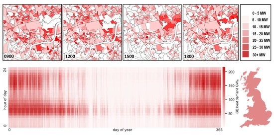
The distinction between overall GB heat load and the urban heat load is made as district heating load would likely be constructed in urban areas owing to the favourable economics. The ratio of domestic to nondomestic heat loads will make a difference to the daily load profile as will the proportion of each archetype, with urban areas having a higher share of flats for example. The heat demand from the top 5% of heat load density MSOAs has been used as a proxy for urban heat load. Figure 11 shows normalized average winter demand profile comparison. The average urban winter load profile has lower peaks and lower peak to trough ratio compared to the average GB load profile which also has a much more pronounced morning peak and a quicker drop-off while the daytime loads from nondomestic building prolong the drop-off to the mid-day trough.
The spatiotemporal load at the LSOA level is shown in Figure at four times (9 am to 6 pm) in Figure 12. The annual values of domestic LSOA load have been calibrated to consumption data, but the inter day profile and nondomestic load at this level are estimated model outputs.
4. Discussion
A high-resolution spatiotemporal Heat Load Model (HeLoM) has been developed to generate estimates of space and water heating demand in urban sub-city areas. Previous studies using similar methods have provided an exploration of domestic loads, but any future large-scale district heating development is unlikely to exclude nondomestic buildings. This model builds on previous work in the segmentation and characterisation of archetypes as well as the construction of a thermal model to derive heat loads. A thermal model using regional weather data has been developed to provide hourly heat loads and can be used to test the efficacy of efficiency interventions in future work.
Knowledge of localised peak loads is necessary when planning electricity infrastructure in the event of large-scale domestic heat pump uptake, but it also has an impact on the design of district heating energy centres. The results of the highest heat demand density areas have been aggregated here as a substitute for total district heating load nationally. The results show that there is a discernible difference in the average heat load profile between the national load profile and the urban subset, which demonstrates the need to disaggregate the urban load. On the national scale, the impact of peak winter heating loads on the electrical system has been the subject of several other studies. This model suggests that the peak may be more likely to occur around the evening peak with the cumulative contribution of domestic and nondomestic demand. The translation of the derived heat loads to heat pump electricity load profiles is open to debate. Heat pumps may be operated with a flatter load profile; therefore, caution should be applied when using these heat loads as a proxy for electrical load and similarly with the use of low temperature district heating demand.
The thermal model contains many simplifications and is not suitable for a more detailed single building analysis where greater construction, orientation, and occupancy detail would be available. The nondomestic archetypes used here were limited to 12 activity classes but could have benefited from data on activity types as well accurate floor area estimates and more monitored occupancy data. This work draws on established building stock modelling methods and building thermal modelling such as BREDEM. The novelty of this study emerges from the combination of the methods and data sources, applied at a high spatial and temporal resolution using historic meteorological data as the main driver of heat demand.
The smallest spatial resolution captured in this model is at the LSOA level and each LSOA can be individually interrogated to obtain heat loads for any given hour. Such a tool has potential for use by urban planners who may want to identify areas of temporal synergy such as whether a residential area with morning and evening peaks is beside a commercial area with day-time load. The results cannot be used for local district heating design, which requires a more localised analysis of heat loads, identifying large heat loads, heat sinks and the loads that differ from the standard occupancy modelled here.
Modelling demand at high resolution necessitates high computing requirements and data storage requirements, particularly as the spatio-temporal resolution increases, more detail needs to be captured. The study has relied on historical consumptions data and a central challenge remains in the validation or calibration of results in the absence of reliable benchmarking data [102].
While the spatial distribution of heat load is unlikely to differ much, there are large uncertainties in future demands from factors such as population growth, efficiency improvements, and climate change effects. While population growth and efficiency improvements can be accounted for in the modelling presented here, climate change may have the biggest impact. The Met Office (REF) UK climate projections envisage a range of 0.7–4.2°C warmer winters by 2070 and more erratic weather patterns whose impact cannot be easily measured. Building efficiency improvements may counteract increases in population growth but more recently we have experienced an upheaval in working patterns and building occupancy in a short period of time. How this might affect absolute demand, day to day temporal variation from weather patterns, and seasonal variation from climate change is still indetermined.
Author Contributions
Conceptualisation, methodology, validation, analysis, data curation, writing—original draft preparation, S.S.; supervision, methodology, analysis, review and editing, M.B.; supervision, review and editing, J.M. All authors have read and agreed to the published version of the manuscript.
Funding
This research was made possible by support from the EPSRC Centre for Doctoral Training in Energy Demand (LoLo), grant numbers EP/L01517X/1 and EP/H009612/1.
Acknowledgments
The Carb2 dataset and building consumption data was kindly provided by Rob Liddiard from the UCL Energy Institute and Penny Challans from Sustainable Energy Ltd. respectively. This research used Valuation Office Agency (VOA) and Office for National Statistics (ONS) data containing public-sector information licensed under the Open Government Licence v1.0.
Conflicts of Interest
The authors declare no conflict of interest. The funders had no role in the design of the study; in the collection, analyses, or interpretation of data; in the writing of the manuscript, or in the decision to publish the results.
Nomenclature
| Qtot | Total heat transfer (W) |
| Qcond | Conduction heat transfer per surface (W) |
| Qconv | Convection heat transfer per surface (W) |
| Qinf | Infiltration heat transfer (W) |
| Qgain | Thermal gains (W) |
| ach | Air Changes per hour |
| Vb | Building volume (m3) |
| Nb | Number of buildings |
| vw | Wind speed (ms−1) |
| U | Thermal transmittance (Wm-2K−1) |
| Tset | Setpoint temperature (K) |
| Text | External wall temperature (K) |
| Tint | Internal wall temperature (K) |
| Tamb | Ambient temperature (K) |
| hc | Wall convection coefficient (Wm−2K−1) |
| As | Wall surface area (m2) |
| Af | Floor area (m2) |
| Ph | Hourly occupancy |
| Mth | Thermal mass (WhK−1) |
| fh | Hourly adjustment factor |
| fm | Monthly adjustment factor |
| Subscripts | Denotes value per surface/wall |
Appendix A

Table A1.
Domestic characterisation: Assumptions and parameters.
| Dwelling Type | Built Period | Floor Area m2 | Height m | Wall U W/m2K | Ground U W/m2K | Loft Floor W/m2K | Glazing U W/m2K | Glazing Trans% | ACH Hour −1 | ∑UA W/K | TMP kJ/m2K | Mth kWh/K | Boiler kW | Mean Occupancy |
|---|---|---|---|---|---|---|---|---|---|---|---|---|---|---|
| Terraced | Pre 1918 | 87 | 4.7 | 2.1 | 0.8 | 0.16 | 3.1 | 0.85 | 0.56 | 311.79 | 612 | 14.8 | 23.95 | 3 |
| Terraced | 1918–1964 | 78 | 4.7 | 2.1 | 0.6 | 0.16 | 3.1 | 0.75 | 0.76 | 294.93 | 500 | 10.8 | 23.02 | 2.9 |
| Terraced | 1965–1980 | 78 | 4.7 | 1.3 | 0.6 | 0.16 | 3.1 | 0.75 | 0.64 | 248.9 | 400 | 8.7 | 20.49 | 2.9 |
| Terraced | 1981–1990 | 68 | 4.7 | 0.6 | 0.6 | 0.3 | 3.1 | 0.75 | 0.64 | 204.77 | 300 | 5.7 | 18.06 | 2.9 |
| Terraced | Post 1990 | 77 | 4.7 | 0.45 | 0.3 | 0.16 | 3.1 | 0.75 | 0.51 | 174.2 | 200 | 4.3 | 16.38 | 2.9 |
| Semi-det | Pre 1918 | 126 | 4.7 | 2.1 | 0.8 | 0.16 | 3.1 | 0.85 | 0.56 | 576.37 | 612 | 21.4 | 33.5 | 3.1 |
| Semi-det | 1918–1964 | 91 | 4.7 | 1.6 | 0.6 | 0.16 | 3.1 | 0.75 | 0.76 | 414.54 | 500 | 12.6 | 26.6 | 3 |
| Semi-det | 1965–1980 | 85.5 | 4.7 | 1.3 | 0.6 | 0.16 | 3.1 | 0.75 | 0.64 | 348.98 | 400 | 9.5 | 21.99 | 3 |
| Semi-det | 1981–1990 | 74 | 4.7 | 0.6 | 0.6 | 0.3 | 3.1 | 0.75 | 0.64 | 255.66 | 300 | 6.2 | 17.86 | 2.9 |
| Semi-det | Post 1990 | 79.5 | 4.7 | 0.45 | 0.3 | 0.16 | 3.1 | 0.75 | 0.51 | 206.1 | 300 | 6.6 | 18.14 | 2.9 |
| Detached | Pre 1918 | 197 | 4.7 | 2.1 | 0.8 | 0.16 | 3.1 | 0.85 | 0.56 | 965.33 | 550 | 30.1 | 49.89 | 2.8 |
| Detached | 1918–1964 | 151 | 4.7 | 1.6 | 0.6 | 0.16 | 3.1 | 0.75 | 0.76 | 720.8 | 450 | 18.9 | 36.44 | 2.3 |
| Detached | 1965–1980 | 135 | 4.7 | 1.3 | 0.6 | 0.16 | 3.1 | 0.75 | 0.64 | 582.68 | 350 | 13.1 | 31.85 | 2.5 |
| Detached | 1981–1990 | 134 | 4.7 | 0.6 | 0.6 | 0.3 | 3.1 | 0.75 | 0.64 | 469.28 | 250 | 9.3 | 32.61 | 2.3 |
| Detached | Post 1990 | 166 | 4.7 | 0.45 | 0.3 | 0.16 | 3.1 | 0.75 | 0.51 | 427.97 | 200 | 9.2 | 37.34 | 2.2 |
| Flat | Pre 1918 | 67 | 2.35 | 2.1 | 0 | 0 | 4.8 | 0.85 | 0.56 | 375.38 | 300 | 5.6 | 27.45 | 2.2 |
| Flat | 1918–1964 | 56 | 2.35 | 2.1 | 0 | 0 | 3.1 | 0.75 | 0.76 | 257.42 | 250 | 3.9 | 20.96 | 1.9 |
| Flat | 1965–1980 | 52.5 | 2.35 | 1.3 | 0 | 0 | 3.1 | 0.75 | 0.64 | 255.75 | 250 | 3.6 | 20.87 | 1.8 |
| Flat | 1981–1990 | 57 | 2.35 | 0.6 | 0 | 0 | 3.1 | 0.75 | 0.64 | 191.39 | 200 | 3.2 | 17.33 | 1.9 |
| Flat | Post 1990 | 60 | 2.35 | 0.45 | 0 | 0 | 3.1 | 0.75 | 0.51 | 141.93 | 200 | 3.3 | 14.61 | 2 |
Table A2.
Nondomestic Archetype parameters used, adapted from [79].
Table A2.
Nondomestic Archetype parameters used, adapted from [79].
| CaRB2 Class | Floor Area m2 | Storey Height m | Depth m | Width Ext% | Glaze % | Glaze Trans% | Glaze Trans% | Wall U W/m2K | Glaze U W/m2K | Roof U W/m2K | Floor U W/m2K | AirCh h−1 | SHL kW/K | Mth kWh/K | Boiler kW | Int Gain W/m2 |
|---|---|---|---|---|---|---|---|---|---|---|---|---|---|---|---|---|
| Office | 276 | 3 | 8 | 0.9 | 0.4 | 0.5 | 0.5 | 1.0. | 3.8 | 0.7 | 0.4 | 3.5 | 1.1 | 19.2 | 19.3 | 32 |
| Shop | 201.7 | 3 | 15 | 0.9 | 0.5 | 0.5 | 0.5 | 1 | 3.8 | 0.7 | 0.4 | 5 | 1.2 | 14 | 20.2 | 46 |
| Factory | 737.3 | 5 | 20 | 0.9 | 0.1 | 0.7 | 0.7 | 1 | 3.8 | 0.7 | 0.4 | 3 | 4.9 | 51.2 | 59 | 90 |
| Warehouse | 922.9 | 8 | 25 | 0.9 | 0.1 | 0.7 | 0.7 | 1 | 3.8 | 0.7 | 0.4 | 1.5 | 5.5 | 64.1 | 46.2 | 27 |
| Hospitality | 365.9 | 3 | 8 | 0.9 | 0.2 | 0.7 | 0.7 | 1 | 3.8 | 0.7 | 0.4 | 5 | 1.9 | 25.4 | 22 | 47 |
| ArtsLeisure | 437.1 | 3 | 8 | 0.9 | 0.2 | 0.7 | 0.7 | 1 | 3.8 | 0.7 | 0.4 | 5 | 2.5 | 30.4 | 43.7 | 30 |
| Sports | 668.6 | 6 | 15 | 0.9 | 0.1 | 0.7 | 0.7 | 1 | 3.8 | 0.7 | 0.4 | 5 | 6.2 | 46.4 | 24.9 | 60 |
| Education | 1291 | 3.5 | 10 | 0.9 | 0.1 | 0.7 | 0.7 | 1 | 3.8 | 0.7 | 0.4 | 3.5 | 6 | 89.7 | 112.3 | 75 |
| Health | 1477.7 | 4 | 15 | 0.9 | 0.2 | 0.7 | 0.7 | 1 | 3.8 | 0.7 | 0.4 | 5 | 7.9 | 102.6 | 73.9 | 69 |
| Transport | 408.2 | 5 | 20 | 0.9 | 0.1 | 0.7 | 0.7 | 1 | 3.8 | 0.7 | 0.4 | 5 | 3.8 | 28.3 | 20.4 | 26 |
| Community | 295.7 | 3 | 7 | 0.9 | 0.1 | 0.7 | 0.7 | 1 | 3.8 | 0.7 | 0.4 | 5 | 1.7 | 20.5 | 20.7 | 40 |
| Emergency | 2496.1 | 4 | 7 | 0.9 | 0.1 | 0.7 | 0.7 | 1 | 3.8 | 0.7 | 0.4 | 5 | 18.6 | 173.3 | 124.8 | 40 |
Table A3.
Details of hourly gas consumption data.
| CaRB2 Class | Building Sources | Data Length | Further Information | Estimated Active Occupancy |
|---|---|---|---|---|
| Offices | 5 | 2011–2015 | 5 office | 7–5 weekday, 8–15 weekend |
| Hospitality | 2 | 2015–2017 | 2 hotels | 6–23 |
| Arts Leisure | 3 | 2013–2014 | 3 theatres | 8–21 |
| Sports | 5 | 2010–2015 | 5 leisure centres | 7–20 |
| Education | 16 | 2011–2015 | 10 primary, 5 sec., 1 college | 6–17 weekday, 6–15 weekend |
| Health | 2 | 2011–2015 | 1 hospital, 2 care homes | 24 h |
| Community | 2 | 2013–2015 | 1 Library, 1 day centre | 7–18 |
| Emergency | 1 | 2013–2014 | Fire station | 24 hr weekday, 12 hr weekend |
Table A4.
Estimated activity classifications.
| CaRB2 Class | Estimated Active Occupancy | Further Information |
|---|---|---|
| Shop (retail) | 9–20 | [88] |
| Factory | 24 h | Reduced overnight |
| Warehouse | 24 h | Reduced overnight |
| Transport | 24 h | Reduced weekend |
Figure A1.
Hourly estimated nondomestic occupancy factors.

Figure A2.
Hourly normalised occupancy factors derived from measured hourly gas consumption.

Figure A3.
Hourly normalised occupancy factors derived from measured hourly gas consumption.

References
- Government of the UK. Climate Change Act C.27; HM Stationary Office: London, UK, 2008.
- Department for Business, Energy & Industrial Strategy (BEIS). Energy White Paper: Powering Our Net Zero Future; Department for Business, Energy & Industrial Strategy: London, UK, 2020.
- Department of Energy & Climate Change (DECC). The Future of Heating: Meeting the Challenge; Department of Energy & Climate Change: London, UK, 2013.
- Department for Business, Energy & Industrial Strategy (BEIS). The Clean Growth Strategy: Leading the Way to a Low Carbon Future; Department for Business, Energy and Industrial Strategy: London, UK, 2017.
- David, A.; Mathiesen, B.V.; Averfalk, H.; Werner, S.; Lund, H. Heat Roadmap Europe: Large-Scale Electric Heat Pumps in District Heating Systems. Energies 2017, 10, 578. [Google Scholar] [CrossRef] [Green Version]
- Wang, Z. Heat Pumps with District Heating for the UK’s Domestic Heating: Individual versus District Level. Energy Procedia 2018, 149, 354–362. [Google Scholar] [CrossRef]
- Ministry of Housing, Communities & Local Government (MHCLG). Conservation of Fuel and Power: Approved Document L.; Ministry of Housing, Communities & Local Government: London, UK, 2014.
- Department for Business, Energy and Industrial Strategy (BEIS). Energy Consumption in the UK; Department for Business, Energy and Industrial Strategy: London, UK, 2020.
- Climate Change Committee. Next Steps for UK Heat Policy; Climate Change Committee: London, UK, 2016; p. 104. [Google Scholar]
- Sousa, G.; Jones, B.M.; Mirzaei, P.A.; Robinson, D. A Review and Critique of UK Housing Stock Energy Models, Modelling Approaches and Data Sources. Energy Build. 2017, 151, 66–80. [Google Scholar] [CrossRef]
- Kavgic, M.; Mavrogianni, A.; Mumovic, D.; Summerfield, A.; Stevanovic, Z.; Djurovic-Petrovic, M. A Review of Bottom-up Building Stock Models for Energy Consumption in the Residential Sector. Build. Environ. 2010, 45, 1683–1697. [Google Scholar] [CrossRef]
- Keirstead, J.; Jennings, M.; Sivakumar, A. A Review of Urban Energy System Models: Approaches, Challenges and Opportunities. Renew. Sustain. Energy Rev. 2012, 16, 3847–3866. [Google Scholar] [CrossRef] [Green Version]
- Reinhart, C.F.; Davila, C.C. Urban Building Energy Modeling—A Review of a Nascent Field. Build. Environ. 2016, 97, 196–202. [Google Scholar] [CrossRef] [Green Version]
- Anderson, B.R. BREDEM-8: Model. Description, 2001 Update; CRC Press: Boca Raton, FL, USA; IHS BRE Pres: Bracknell, UK, 2002; ISBN 9781860815379. [Google Scholar]
- Henderson, J.; Hart, J. BREDEM 2012—A Technical Description of the BRE Domestic Energy Model; BRE: Watford, UK, 2013. [Google Scholar]
- Firth, S.K.; Lomas, K.J.; Wright, A.J. Targeting Household Energy-Efficiency Measures Using Sensitivity Analysis. Build. Res. Inf. 2010, 38, 25–41. [Google Scholar] [CrossRef] [Green Version]
- Eggimann, S.; Hall, J.W.; Eyre, N. A High-Resolution Spatio-Temporal Energy Demand Simulation to Explore the Potential of Heating Demand Side Management with Large-Scale Heat Pump Diffusion. Appl. Energy 2019, 236, 997–1010. [Google Scholar] [CrossRef]
- Clegg, S.; Mancarella, P. Integrated Electricity-Heat-Gas Modelling and Assessment, with Applications to the Great Britain System—Part II: Transmission Network Analysis and Low Carbon Technology and Resilience Case Studies. Energy 2019, 184, 191–203. [Google Scholar] [CrossRef] [Green Version]
- Wang, H.; Mancarella, P. Towards Sustainable Urban Energy Systems: High Resolution Modelling of Electricity and Heat Demand Profiles. In Proceedings of the 2016 IEEE International Conference on Power System Technology (POWERCON), Wollongong, Australia, 28 September–1 October 2016; pp. 1–6. [Google Scholar]
- Taylor, S.; Firth, S.K.; Wang, C.; Allinson, D.; Quddus, M.; Smith, P. Spatial Mapping of Building Energy Demand in Great Britain. GCB Bioenergy 2014, 6, 123–135. [Google Scholar] [CrossRef] [Green Version]
- Quiggin, D.; Buswell, R. The Implications of Heat Electrification on National Electrical Supply-Demand Balance under Published 2050 Energy Scenarios. Energy 2016, 98, 253–270. [Google Scholar] [CrossRef] [Green Version]
- Sansom, R. Decarbonising Low Grade Heat for Low Carbon Future. Ph.D. Thesis, Imperial College London, London, UK, 2014. [Google Scholar] [CrossRef]
- Bruhns, H.; Steadman, P.; Herring, H. A Database for Modeling Energy Use in the Non-Domestic Building Stock of England and Wales. Appl. Energy 2000, 66, 277–297. [Google Scholar] [CrossRef]
- Liddiard, R.; Wright, A.; Marjanovic-Halburd, L. A Review of Non-Domestic Energy Benchmarks and Benchmarking Methodologies. In Proceedings of the 5th International Conference on Improving Energy Efficiency in Commercial Buildings IEECB Focus, Frankfurt, Germany, 10–11 April 2008. [Google Scholar]
- Smith, S.T. Modelling Thermal Loads for a Non-Domestic Building Stock: Associating a Priori Probability with Building Form and Construction—Using Building Control Laws and Regulations. Ph.D. Thesis, University of Nottingham, Nottingham, UK, 2009. [Google Scholar]
- Steadman, P. The Non-Domestic Building Stock of England and Wales. In Structure and Style; Taylor and Francis Group: Abingdon, UK, 1997. [Google Scholar]
- Cheng, V.; Steemers, K. Modelling Domestic Energy Consumption at District Scale: A Tool to Support National and Local Energy Policies. Environ. Model. Softw. 2011, 26, 1186–1198. [Google Scholar] [CrossRef]
- Ministry of Housing, Communities and Local Government. English Housing Survey, 2017: Housing Stock Data; [data collection], SN: 8494; UK Data Service: Colchester, UK, 2017. [CrossRef]
- Department for Business, Energy & Industrial Strategy (BEIS). Cambridge Housing Model and User Guide; Department for Business, Energy & Industrial Strategy: London, UK, 2010.
- Building Research Establishment. The Government’s Standard Assessment Procedure for Energy Rating of Dwellings (SAP); 2005 Edition; Building Research Establishment: London, UK, 2009.
- Arababadi, R. Energy Use in the EU Building Stock; Case Study; Linkoping University: Linkoping, Sweden, 2012. [Google Scholar]
- Rylatt, R.M.; Gadsden, S.J.; Lomas, K.J. Methods of Predicting Urban Domestic Energy Demand with Reduced Datasets: A Review and a New GIS-Based Approach. Build. Serv. Eng. Res. Technol. 2003, 24, 93–102. [Google Scholar] [CrossRef]
- Oikonomou, E.; Davies, M.; Mavrogianni, A.; Biddulph, P.; Wilkinson, P.; Kolokotroni, M. Modelling the Relative Importance of the Urban Heat Island and the Thermal Quality of Dwellings for Overheating in London. Build. Environ. 2012, 57, 223–238. [Google Scholar] [CrossRef]
- Yao, R.; Steemers, K. A Method of Formulating Energy Load Profile for Domestic Buildings in the UK. Energy Build. 2005, 37, 663–671. [Google Scholar] [CrossRef]
- Calderón, C.; James, P.; Urquizo, J.; McLoughlin, A. A GIS Domestic Building Framework to Estimate Energy End-Use Demand in UK Sub-City Areas. Energy Build. 2015, 96, 236–250. [Google Scholar] [CrossRef] [Green Version]
- Rosser, J.F.; Long, G.; Zakhary, S.; Boyd, D.S.; Mao, Y.; Robinson, D. Modelling Urban Housing Stocks for Building Energy Simulation Using CityGML EnergyADE. ISPRS Int. J. Geo. Inf. 2019, 8, 163. [Google Scholar] [CrossRef] [Green Version]
- Watson, S.D.; Lomas, K.J.; Buswell, R.A. Decarbonising Domestic Heating: What Is the Peak GB Demand? Energy Policy 2019, 126, 533–544. [Google Scholar] [CrossRef]
- Evans, S.; Liddiard, R.; Steadman, P. 3DStock: A New Kind of Three-Dimensional Model of the Building Stock of England and Wales, for Use in Energy Analysis. Environ. Plan B Urban Anal. City Sci. 2017, 44, 227–255. [Google Scholar] [CrossRef] [Green Version]
- Department for Business, Energy and Industrial Strategy (BEIS). Building Energy Efficiency Survey (BEES); Department for Business, Energy and Industrial Strategy: London, UK, 2016.
- Steadman, P.; Evans, S.; Liddiard, R.; Godoy-Shimizu, D.; Ruyssevelt, P.; Humphrey, D. Building Stock Energy Modelling in the UK: The 3DStock Method and the London Building Stock Model. Build. Cities 2020, 1, 100–119. [Google Scholar] [CrossRef]
- Liddiard, R. CaRB2. Available online: https://www.ucl.ac.uk/energy-models/models/carb2 (accessed on 1 February 2021).
- Armitage, P.; Godoy-Shimizu, D.; Palmer, J. The Cambridge Non-Domestic Energy Model; Technical Report; Cambridge Energy: Cambridge, UK, 2015; p. 11. [Google Scholar]
- Taylor, S.; Fan, D.; Rylatt, M. Enabling Urban-Scale Energy Modelling: A New Spatial Approach. Build. Res. Inf. 2014, 42, 4–16. [Google Scholar] [CrossRef]
- Centre for Sustainable Energy. National Heat Map. Available online: https://www.cse.org.uk/projects/view/1183 (accessed on 3 February 2021).
- Fremouw, M. Quantifying Urban Energy Potentials: Presenting Three European Research Projects. In Proceedings of the P Smart & Sustainable Cities and Transport Seminar (CSIR), Pretoria, South Africa, 12–14 July 2017. [Google Scholar]
- Prieto, I.; Sonvilla, P.M.; Munguet, M.C.; Wilson, J.; Kesik, M.; Rieksts-Riekstins, V.; Wenzel, T.; Dinis, J.; Wyke, S.; Seeman, M.-E. THERMOS—Baseline Replication Assessment Report; European Commission: Brussels, Belgium, 2018. [Google Scholar]
- Robinson, D.; Haldi, F.; Leroux, P.; Perez, D.; Rasheed, A.; Wilke, U. CitySim: Comprehensive Micro-Simulation of Resource Flows for Sustainable Urban Planning. In Proceedings of the Eleventh International IBPSA Conference, Glasgow, Scotland, 27–30 July 2009; pp. 1083–1090. [Google Scholar]
- Huber, J.; Nytsch-Geusen, C. Development of Modeling and Simulation Strategies for Large-Scale Urban Districts. In Proceedings of the Building Simulation IBPSA 2011, Sydney, Australia, 14–16 November 2011; pp. 1753–1760. [Google Scholar]
- Calikus, E.; Nowaczyk, S.; Sant’Anna, A.; Gadd, H.; Werner, S. A Data-Driven Approach for Discovering Heat Load Patterns in District Heating. Appl. Energy 2019, 252, 113409. [Google Scholar] [CrossRef]
- Dahl, M.; Brun, A.; Andresen, G.B. Using Ensemble Weather Predictions in District Heating Operation and Load Forecasting. Appl. Energy 2017, 193, 455–465. [Google Scholar] [CrossRef]
- Dalipi, F.; Yildirim Yayilgan, S.; Gebremedhin, A. Data-Driven Machine-Learning Model in District Heating System for Heat Load Prediction: A Comparison Study. Appl. Comput. Intell. Soft Comput. 2016, 2016, 1–11. [Google Scholar] [CrossRef] [Green Version]
- Guelpa, E.; Marincioni, L.; Capone, M.; Deputato, S.; Verda, V. Thermal Load Prediction in District Heating Systems. Energy 2019, 176, 693–703. [Google Scholar] [CrossRef]
- Idowu, S.; Saguna, S.; Åhlund, C.; Schelen, O. Applied Machine Learning: Forecasting Heat Load in District Heating System. Energy Build. 2016, 133, 478–488. [Google Scholar] [CrossRef]
- Mikkola, J.; Lund, P.D. Models for Generating Place and Time Dependent Urban Energy Demand Profiles. Appl. Energy 2014, 130, 256–264. [Google Scholar] [CrossRef]
- Nouvel, R.; Mastrucci, A.; Leopold, U.; Baume, O.; Coors, V.; Eicker, U. Combining GIS-Based Statistical and Engineering Urban Heat Consumption Models: Towards a New Framework for Multi-Scale Policy Support. Energy Build. 2015, 107, 204–212. [Google Scholar] [CrossRef]
- Dogan, T.; Reinhart, C. Shoeboxer: An Algorithm for Abstracted Rapid Multi-Zone Urban Building Energy Model Generation and Simulation. Energy Build. 2017, 140, 140–153. [Google Scholar] [CrossRef]
- Nageler, P.; Zahrer, G.; Heimrath, R.; Mach, T.; Mauthner, F.; Leusbrock, I.; Schranzhofer, H.; Hochenauer, C. Novel Validated Method for GIS Based Automated Dynamic Urban Building Energy Simulations. Energy 2017, 139, 142–154. [Google Scholar] [CrossRef]
- Mata, E.; Sasic Kalagasidis, A.; Johnsson, F. Building-Stock Aggregation through Archetype Buildings: France, Germany, Spain and the UK. Build. Environ. 2014, 81, 270–282. [Google Scholar] [CrossRef] [Green Version]
- Valuation Office Agency VOA. 2020. Available online: https://data.gov.uk/dataset/22cea4d7-d0ce-4b8d-8df3-45cc52ef4ae5/voa-non-domestic-rating-addresses-floor-areas-characteristics-and-attributes-of-properties (accessed on 5 July 2021).
- Scottish Government Statistics. Small Area Statistics on Households and Dwellings. Available online: https://statistics.gov.scot/ (accessed on 1 June 2020).
- Office for National Statistics. Census Statistics; Office for National Statistics: London, UK, 2020.
- Department for Business, Energy & Industrial Strategy (BEIS). Sub-National Gas—Consumption Data; Department for Business, Energy & Industrial Strategy: London, UK, 2020.
- Scottish Government. Scotland’s Non-Domestic Energy Efficiency Baseline; Scottish Government: Edinburgh, Scotland, 2018.
- Met Office. MIDAS Open: UK Land Surface Stations Data (1853–Current); Centre for Environmental Data Analysis: Oxfordshire, UK, 2019.
- Ministry of Housing, Communities & Local Government (MHCLG). English Housing Survey; Ministry of Housing, Communities & Local Government: London, UK, 2016.
- Stamp, S.F. Assessing Uncertainty in Co-Heating Tests: Calibrating a Whole Building Steady State Heat Loss Measurement Method. Ph.D. Thesis, University College London (UCL), London, UK, 2016. [Google Scholar]
- Boswarva, O. Profiling the Age of Housing Stock in England and Wales. Available online: https://www.owenboswarva.com/blog/archive/mg/20161213.htm (accessed on 7 June 2021).
- Piddington, J.; Nicol, S.; Garret, H.; Custard, M. The Housing Stock of The United Kingdom; BRE Trust: Watford, UK, 2020. [Google Scholar]
- Buttitta, G.; Turner, W.J.N.; Neu, O.; Finn, D.P. Development of Occupancy-Integrated Archetypes: Use of Data Mining Clustering Techniques to Embed Occupant Behaviour Profiles in Archetypes. Energy Build. 2019, 198, 84–99. [Google Scholar] [CrossRef]
- Ministry of Housing, Communities & Local Government (MHCLG). English Housing Survey—Floor Space in English Homes—Main Report; Ministry of Housing, Communities & Local Government: London, UK, 2018.
- Building Research Establishment (BRE). The Government’s Standard Assessment Procedure for Energy Rating of Dwellings (SAP 2016); Building Research Establishment: Watford, UK, 2016. [Google Scholar]
- Palmer, J.; Cooper, I. United Kingdom Housing Energy Fact File; Department of Energy and Climate Change: London, UK, 2013; p. 146.
- Energy Saving Trust. CE54: Domestic Heating Sizing Method. 2010. Available online: https://www.eogb.co.uk/ce54-domestic-heating-sizing-method/ (accessed on 11 January 2021).
- Hanmer, C.; Shipworth, M.; Shipworth, D.; Carter, E. How Household Thermal Routines Shape UK Home Heating Demand Patterns. Energy Effic. 2019, 12, 5–17. [Google Scholar] [CrossRef] [Green Version]
- Love, J.; Smith, A.Z.P.; Watson, S.; Oikonomou, E.; Summerfield, A.; Gleeson, C.; Biddulph, P.; Chiu, L.F.; Wingfield, J.; Martin, C.; et al. The Addition of Heat Pump Electricity Load Profiles to GB Electricity Demand: Evidence from a Heat Pump Field Trial. Appl. Energy 2017, 204, 332–342. [Google Scholar] [CrossRef]
- Wang, Z.; Crawley, J.; Li, F.G.N.; Lowe, R. Sizing of District Heating Systems Based on Smart Meter Data: Quantifying the Aggregated Domestic Energy Demand and Demand Diversity in the UK. Energy 2020, 193, 116780. [Google Scholar] [CrossRef]
- Liddiard, R.; UCL Energy Institute, London, UK. Personal communication, 2020.
- Department for Communities and Local Government (DCLG). Zero Carbon Non-Domestic Buildings: Phase 3 Final Report; Department for Communities and Local Government: London, UK, 2011; ISBN 978-1-4098-3001-6.
- Barrett, M.; Research at Propeller HealthSan, Francisco, CA, USA. Personal communication, 2020.
- Gakovic, B. Areas and Types of Glazing and Other Openings in the Nondomestic Building Stock. Environ. Plan. B Plan. Des. 2000, 27, 667–694. [Google Scholar] [CrossRef]
- Steadman, P.; Evans, S.; Batty, M. Wall Area, Volume and Plan Depth in the Building Stock. Build. Res. Inf. 2009, 37, 455–467. [Google Scholar] [CrossRef] [Green Version]
- Steadman, P.; Bruhns, H.R.; Gakovic, B. Inferences about Built Form, Construction, and Fabric in the Nondomestic Building Stock of England and Wales. Environ. Plan. B Plan. Des. 2000, 27, 733–758. [Google Scholar] [CrossRef]
- Hawkins, G. Rules of Thumb: Guidelines for Building Services; BSRIA: Bracknell, UK, 2011; ISBN 978-0-86022-691-8. [Google Scholar]
- Chartered Institution of Building Services Engineers. Environmental Design: CIBSE Guide A, Chapter 6, 8th ed.; CIBSE Guide; Chartered Institution of Building Services Engineers: London, UK, 2015; ISBN 978-1-906846-54-1. [Google Scholar]
- Korolija, I.; Marjanovic-Halburd, L.; Zhang, Y.; Hanby, V.I. UK Office Buildings Archetypal Model as Methodological Approach in Development of Regression Models for Predicting Building Energy Consumption from Heating and Cooling Demands. Energy Build. 2013, 60, 152–162. [Google Scholar] [CrossRef]
- Tian, W.; Choudhary, R. A Probabilistic Energy Model for Non-Domestic Building Sectors Applied to Analysis of School Buildings in Greater London. Energy Build. 2012, 54, 1–11. [Google Scholar] [CrossRef] [Green Version]
- Challans, P. Hourly and Half Hourly Gas Data; Private Message; Sustainable Energy Limited: Hong Kong, China, 2018. [Google Scholar]
- Duarte, C.; Van Den Wymelenberg, K.; Rieger, C. Revealing Occupancy Patterns in an Office Building through the Use of Occupancy Sensor Data. Energy Build. 2013, 67, 587–595. [Google Scholar] [CrossRef]
- Lindberg, K.B.; Bakker, S.J.; Sartori, I. Modelling Electric and Heat Load Profiles of Non-Residential Buildings for Use in Long-Term Aggregate Load Forecasts. Util. Policy 2019, 58, 63–88. [Google Scholar] [CrossRef]
- Shipworth, M.; Firth, S.K.; Gentry, M.I.; Wright, A.J.; Shipworth, D.T.; Lomas, K.J. Central Heating Thermostat Settings and Timing: Building Demographics. Build. Res. Inf. 2010, 38, 50–69. [Google Scholar] [CrossRef] [Green Version]
- Palyvos, J.A. A Survey of Wind Convection Coefficient Correlations for Building Envelope Energy Systems’ Modeling. Appl. Therm. Eng. 2008, 28, 801–808. [Google Scholar] [CrossRef]
- Chartered Institution of Building Services Engineers. Guide C: Reference Data, 8th ed.; CIBSE Guide; Chartered Institution of Building Services Engineers: London, UK, 2007; ISBN 978-1-906846-54-1. [Google Scholar]
- Grant, N.; Clarke, A. Internal Gain Assumptions and Building Size. In Proceedings of the 18th International Passivhaus Conference, Aachen, Germany, 25–26 April 2014; p. 599. Available online: https://shop.passivehouse.com/en/products/ende-conference-proceedingstagungsband-18th-international-passive-house-conference-23/ (accessed on 6 July 2021).
- Chartered Institution of Building Services Engineers (CIBSE). Heat Networks: Code of Practice for the UK; Chartered Institution of Building Services Engineers: London, UK, 2015. [Google Scholar]
- Fuentes, E.; Arce, L.; Salom, J. A Review of Domestic Hot Water Consumption Profiles for Application in Systems and Buildings Energy Performance Analysis. Renew. Sustain. Energy Rev. 2018, 81, 1530–1547. [Google Scholar] [CrossRef]
- Energy Saving Trust (EST). Measurement of Domestic Hot Water Consumption in Dwellings; Department for Environment, Food and Rural Affairs, Energy Saving Trust: London, UK, 2008.
- Knight, I.; Kreutzer, N.; Manning, M.; Swinton, M.; Ribberink, H. European and Canadian Non-HVAC Electric and DHW Load Profiles for Use in Simulating the Performance of Residential Cogeneration Systems; A Report of Subtask A of FC+ COGEN-SIM: The Simulation of Building-Integrated Fuel Cell and Other Cogeneration Systems: Annex 42 of the International Energy Agency; Energy Conservation in Buildings and Community Systems Programme, IEA: Paris, France, 2007. [Google Scholar]
- Robinson, I. Design Guide: Stored Hot Water Solutions in Heat Networks; Hot Water Association: Kenilworth, UK, 2018. [Google Scholar]
- Burzynski, R.; Crane, M.; Yao, R.; Becerra, V. Space Heating and Hot Water Demand Analysis of Dwellings Connected to District Heating Scheme in UK. J. Cent. South Univ. Technol. 2012, 19, 1629–1638. [Google Scholar] [CrossRef]
- Department for Business, Energy and Industrial Strategy (BEIS). Business Energy Statistical Summary: How Energy Is Used and by Whom in the Non-Domestic Sector; Department for Business, Energy and Industrial Strategy: London, UK, 2018.
- Imam, S.; Coley, D.A.; Walker, I. The Building Performance Gap: Are Modellers Literate? Build. Serv. Eng. Res. Technol. 2017, 38, 351–375. [Google Scholar] [CrossRef] [Green Version]
- Oreszczyn, T.; Lowe, R. Challenges for Energy and Buildings Research: Objectives, Methods and Funding Mechanisms. Build. Res. Inf. 2010, 38, 107–122. [Google Scholar] [CrossRef]
Figure 1.
Dwelling types in the UK housing stock.

Figure 2.
Dwelling built period in the UK housing stock, adapted from [68].
Figure 2.
Dwelling built period in the UK housing stock, adapted from [68].

Figure 3.
Normalised domestic occupancy profile.

Figure 4.
Count and floor area per activity classification in the CaRB2 database.

Figure 5.
Proportion of nondomestic archetypes in modelled urban areas.

Figure 6.
Nondomestic classification share in Scotland, adapted from [63].
Figure 6.
Nondomestic classification share in Scotland, adapted from [63].

Figure 7.
Normalised hourly domestic hot water load profiles.

Figure 8.
Sensitivity of parameters in thermal model.

Figure 9.
Modelled GB hourly heat demand for 2010.

Figure 10.
Mean winter load profile comparison of GB December average and coldest day.

Figure 11.
Average winter load profile comparison.

Figure 12.
Spatiotemporal variation of modelled heat load for a sub-city area in London.

Table 1.
Summary of data sources.
| Data | Level | Source |
|---|---|---|
| Dwelling build period | LSOA/DZ | CTSOP4.1 [59,60] |
| Dwelling type | LSOA/DZ | QS402EW [61] QS402SC [60] |
| Domestic Heating type | LSOA/DZ | QS415EW [61] QS415SC [60] |
| UK Domestic and Nondomestic Gas Consumption | LSOA/DZ MSOA/IZ | Subnational Gas consumption [62] |
| Nondomestic floor areas | Building | CaRB2 from [59,63] |
| Standard Area measurements | MSOA/IZ | ONS Census [61] Scottish Census [60] |
| Weather data | Regional | Met Office MIDAS [64] |
Table 2.
Archetypes used in comparative studies.
| Source | Dwelling Types | Age Categories | Geographic Zones |
|---|---|---|---|
| Mata et al. [58] | 6 Domestic 3 Nondomestic | 8 pre-1985 to post-2010 | 4—major cities |
| Cheng and Steemers [27] | 5 | 10 pre-1900 to post-2000 | 1—using 30 year mean data |
| Buttita et al. [69] | 5 with multiple variations | 5 pre-1918 to post-1991 | 4—major cities |
| Oikonomou et al. [33] | 5 with multiple variations | 6 | 1—52 sites in London |
| Stamp [66] | 4 | 4 construction styles | 3 weather files |
| HeLoM | 4 | 5 | 11—GB regions |
Table 3.
Domestic archetype data sources.
| Parameter | Source |
|---|---|
| Dwelling Geometry | English Housing Survey [70] |
| Construction U-values, Air tightness | BREDEM 2012 [15] |
| Thermal Mass Parameter | Stamp [66] |
| Boiler/Heating system size | CE54 [73] |
| Glazing transmittance | SAP 2016 [71] |
Table 4.
UK hourly weather observation—Regional stations.
| Region | Station ID | Station Name |
|---|---|---|
| London | 708 | Heathrow |
| South East | 795 | Shorham Airport |
| 862 | Hampshire (Solar observation) | |
| South West | 676 | Filton |
| East of England | 461 | Bedford |
| East Midlands | 554 | Sutton Bonington |
| West Midlands | 19,187 | Coleshill |
| North West | 1119 | Stonyhurst |
| 1083 | Shap (Solar observation) | |
| Yorkshire and the Humber | 534 | Bramham |
| 370 | Leconfield (Solar observation) | |
| North East | 326 | Durham |
| Wales | 19,206 | St Athan |
| Scotland | 24,125 | Glasgow Bishopton |
Table 5.
Monthly factor for domestic hot water variation [99].
Table 5.
Monthly factor for domestic hot water variation [99].
| Jan | Feb | Mar | Apr | May | Jun | Jul | Aug | Sep | Oct | Nov | Dec | |
|---|---|---|---|---|---|---|---|---|---|---|---|---|
| fm | 1.10 | 1.06 | 1.02 | 0.98 | 0.94 | 0.90 | 0.90 | 0.94 | 0.98 | 1.02 | 1.06 | 1.10 |
Table 6.
Average calibration factors per region.
| Region | LSOAs Modelled | Modelled LSOAs with above 50% Domestic Gas Connection | Mean Calibration Factor (Modelled/Measured) |
|---|---|---|---|
| London | 3443 | 2047 | 0.92 |
| South East | 906 | 654 | 1.01 |
| South West | 353 | 215 | 0.99 |
| East of England | 405 | 337 | 1.10 |
| East Midlands | 449 | 389 | 1.09 |
| West Midlands | 919 | 829 | 1.15 |
| North West | 1002 | 856 | 1.13 |
| Yorkshire and the Humber | 723 | 646 | 1.09 |
| North East | 357 | 324 | 1.11 |
| Wales | 181 | 146 | 1.07 |
| Scotland | 1051 | 764 | 0.94 |
| Total | 9789 | 7207 | 1.03 |
Table 7.
Comparison of 2010 heat load with previous estimates.
| Model | Domestic Annual TWh | Domestic Peak GWth | ND Annual TWh | Total Peak GWth |
|---|---|---|---|---|
| HeLoM | 362 | 172 | 124 | 219 |
| Watson et al. [37] | 391 | 170 | - | - |
| Sansom [22] | 398 | 277 | 144 | 358 |
| Quiggin and Buswell [21] | 358 | 262/117 | 105 | - |
Table 8.
ECUK 2010 heating consumption estimates (DECC 2015).
| 2010 | Domestic TWh | Industrial TWh | Service TWh | Total Nondom TWh | Total TWh |
|---|---|---|---|---|---|
| Space Heating | 401 | 35 | 114 | 149 | 550 |
| Hot Water | 82 | - | 22 | 22 | 104 |
| Total | 483 | 35 | 136 | 171 | 654 |
Publisher’s Note: MDPI stays neutral with regard to jurisdictional claims in published maps and institutional affiliations. |
© 2021 by the authors. Licensee MDPI, Basel, Switzerland. This article is an open access article distributed under the terms and conditions of the Creative Commons Attribution (CC BY) license (https://creativecommons.org/licenses/by/4.0/).
Share and Cite
MDPI and ACS Style
Siddiqui, S.; Barrett, M.; Macadam, J. A High Resolution Spatiotemporal Urban Heat Load Model for GB. Energies 2021, 14, 4078. https://doi.org/10.3390/en14144078
AMA Style
Siddiqui S, Barrett M, Macadam J. A High Resolution Spatiotemporal Urban Heat Load Model for GB. Energies. 2021; 14(14):4078. https://doi.org/10.3390/en14144078
Chicago/Turabian StyleSiddiqui, Salman, Mark Barrett, and John Macadam. 2021. "A High Resolution Spatiotemporal Urban Heat Load Model for GB" Energies 14, no. 14: 4078. https://doi.org/10.3390/en14144078
Note that from the first issue of 2016, this journal uses article numbers instead of page numbers. See further details here.