Abstract
It is well known that the water hammer phenomenon can lead to pipeline system failures. For this reason, there is an increased need for simulation of hydraulic transients. High-density polyethylene (HDPE) pipes are commonly used in various pressurised pipeline systems. Most studies have only focused on water hammer events in a single pipe. However, typical fluid distribution networks are composed of serially connected pipes with various inner diameters. The present paper aims to investigate the influence of sudden cross-section changes in an HDPE pipeline system on pressure oscillations during the water hammer phenomenon. Numerical and experimental studies have been conducted. In order to include the viscoelastic behaviour of the HDPE pipe wall, the generalised Kelvin–Voigt model was introduced into the continuity equation. Transient equations were numerically solved using the explicit MacCormack method. A numerical model that involves assigning two values of flow velocity to the connection node was used. The aim of the conducted experiments was to record pressure changes downstream of the pipeline system during valve-induced water hammer. In order to validate the numerical model, the simulation results were compared with experimental data. A satisfactory compliance between the results of the numerical calculations and laboratory data was obtained.
1. Introduction
High-density polyethylene (HDPE) pipes are widely used in various pressurised pipeline systems. This is due to the excellent mechanical and chemical properties of polymers. Almost without exception, polymeric materials are known to exhibit time-dependent viscoelastic mechanical behaviour [1]. This property is particularly visible in the case of hydraulic transients, as it induces major dissipation and dispersion of the pressure waves [2]. In many practical applications, accurate computational models predicting pressure oscillations in pipeline systems are required [3]. For this reason, several studies investigating pipe wall behaviour during the water hammer phenomenon have been conducted. Most of the papers on this topic refer to single-pipe systems [4,5,6,7,8,9]. However, typical fluid distribution networks are composed of serially connected pipes with various inner diameters. Transients in viscoelastic pipes with sudden contractions and expansions have seldom been addressed in the literature. To the authors’ knowledge, only [10] investigated the influence of cross-section changes on pressure waves, and [11] studied transients in a series of two polymeric pipes. Recently, in order to numerically simulate water hammer in steel pipe series, an improved junction boundary condition was established [12]. It involves assigning two sets of values, which describe flow parameters, to the connection node, thus causing it to act as two separate nodes. The present paper aims to confirm this method for HDPE pipes. As part of the study, laboratory tests were conducted, designed to record pressure changes at the downstream end of a serially connected HDPE pipeline system. To numerically solve the transient flow equations, the MacCormack explicit scheme was used. The results of the numerical calculations were compared with the experimental data.
This article is organised as follows. After this introduction, the second section gives a brief overview of the theoretical aspects of the viscoelastic behaviour of the pipe structure. In the third section, a one-dimensional numerical model of the water hammer phenomenon in serially connected viscoelastic pipes is presented. The next section looks at the experimental study. Analysis of the experimental data and numerical model validation are presented in the fifth section, and some conclusions are drawn in the final section.
2. Transient Flow Equations in Viscoelastic Pipelines
The standard system describing the one-dimensional transient flow of a compressible liquid in an elastic pipe consists of the continuity Equation (1) and momentum Equation (2) [13,14]:
where f is the friction factor, c is the pressure wave velocity, h is the piezometric head, v is the average flow velocity, g is the gravity acceleration, x is the space coordinate, t is time and D is the internal pipe diameter.
The system of Equations (1) and (2) may be applied for steel pipelines. However, this mathematical description is no longer suitable when transient flow in polymeric pipes is considered. Polymers exhibit both viscous and elastic characteristics. In practice, to include the viscoelastic behaviour of the pipe wall during transient flow, the approach of “mechanical analogues” is usually used. In this approach, the one-dimensional mechanical response of an elastic solid is represented by the mechanical analogue of a spring, and the linear viscous response is represented by a viscous dashpot [15] (Figure 1).
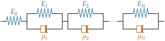
Figure 1.
Generalised Kelvin–Voigt model.
Figure 1 shows the so-called generalised Kelvin–Voigt model, which consists of N elements. The total strain can be described as a sum of instantaneous (elastic) strain and retarded strain [4,5]:
where ε0 is the instantaneous (elastic) strain and εr is the retarded strain. The total retarded strain results from the behaviour of each of the N elements:
The total strain generated by the constant stress is as follows:
where σ is the constant applied stress, E0 is the elastic bulk modulus of the spring, Ek is the elastic bulk modulus of the k-th Kelvin–Voigt element, τk is the retardation time of the k-th Kelvin–Voigt element defined by τk = μk/Ek and ƒ⊂k is the viscosity of the k-th dashpot.
The creep compliance function corresponding to the generalised Kelvin–Voigt model is equal to the following:
where J0 is the instantaneous creep compliance of the first spring, defined by J0 = 1/E0, and Jk is the creep compliance of the k-th Kelvin–Voigt element, defined by Jk = 1/Ek.
According to the Boltzmann superposition principle, the total strain is as follows:
where ξ is a dummy parameter required for integration.
The hoop stress is related to pipe wall thickness and internal diameter:
where α is a dimensionless parameter (dependent on pipe diameter and constraints), s is the pipe wall thickness, p is the current pressure and p0 is the steady-state pressure.
After calculating the creep function time derivative in Equation (7) and including Equation (8) in it, one obtains the following:
This strain influences the cross-sectional area of the pipe, and therefore, it must be included in the continuity equation. In order to take into account the viscoelastic properties of the polymer pipe, the continuity Equation (1) has to be derived from the Reynolds transport theorem [16]. The final form of the continuity equation is as follows:
Equations (2) and (10) constitute the mathematical description of transient flow in a polymeric pipe. A separate problem is how friction is represented in the momentum Equation (2). The way of representing friction in Equation (2) has a significant impact on the results of the numerical calculations of the water hammer equations [17]. The most common approach is to include one of the many unsteady friction models in the continuity equation [18,19]. However, the problem of unsteady friction falls outside the scope of this investigation, as energy dissipation was taken into account by applying a viscoelastic model, and the friction factor was calculated using the Darcy–Weisbach equation:
where fs is the Darcy friction factor.
3. Numerical Solution of Transient Flow Equations
In order to numerically solve the set of Equations (2) and (10), the MacCormack predictor–corrector finite difference explicit scheme was used [20,21]. This method is widely used in computational fluid dynamics [22], but it was only recently adapted to simulate water hammer in elastic pipes by [23] and also successfully used in [24]. In this model, the time step is no longer subjected to the spatial step, and thus, it is more convenient for meshing variable property series pipes than the classic method of characteristics is. The numerical grid was divided into sections that represent individual pipes with given properties. This allows for assigning different values of input data corresponding to each pipe (i.e., inner diameter, creep compliance, retardation time, number of Kelvin–Voigt elements). The pressure wave travels in the pipeline through the junction node connecting individual pipes. To illustrate the discretisation scheme and solving process, a numerical mesh is shown in Figure 2.
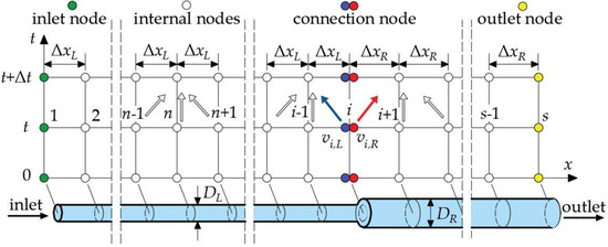
Figure 2.
Numerical grid for the MacCormack explicit scheme.
Furthermore, subscripts denoting different types of numerical nodes are as in Figure 2.
- -
- Inlet boundary condition
For a pipe connected to a constant head reservoir, the boundary condition for the first node is as follows:
where Δt is the time step and h0 is the initial head.
- -
- Outlet boundary condition
For a closed valve, the outlet condition is defined as follows:
Using the backward difference, the outlet boundary condition can be calculated:
- -
- Internal nodes
The derivation of the similar numerical discrete format for the internal nodes of the elastic pipeline system is in [12]. Here, Equations (1) and (10) are presented in basic time-marching format only:
The retarded strain in Equation (10) is calculated as a sum of each Kelvin–Voigt element:
Discrete approximation of each retarded strain is equal to the following:
with the function F at time t-∆t described as follows:
It should be noted that in this numerical model, the constant value of the pressure wave velocity describes the velocity of the transient wave travelling through the entire pipeline system.
- -
- Connection node
In order to take into account any sudden change in the pipeline cross-section, the earlier established connection node condition was used. It involves assigning two sets of values describing the flow parameters to the connection node, which causes it to act as two separate nodes (Figure 2). The detailed derivation of the junction boundary condition is described in [12]. Here, only the final equations are given for brevity. The relation between the flow velocity on the left-hand side of the connection node and the value of the flow velocity on the right-hand side of the connection node is given by:
where vi,L is the velocity on the left-hand side of the connection node, vi,R is the velocity on the right-hand side of the connection node, DL is the inner diameter of the pipe on the left-hand side of the connection node and DR is the inner diameter of the pipe on the right-hand side of the connection node.
Equation (21) is a cubic function, so it has three roots, only one of which satisfies the physical conditions. After computing the value of the flow velocity on the left-hand side of the connection node vi,L, the value of the flow velocity on the right-hand side of the connection node vi,R was calculated with the following:
4. Experimental Study
The goal of the conducted experiments was to obtain the pressure changes during the rapid water hammer phenomenon at the downstream end of a viscoelastic pipeline system with sudden contractions and expansions. Experimental data were later used to validate the numerical model. Four types of experiments were conducted (Figure 3).
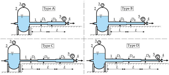
Figure 3.
Experimental setup.
The main elements of the experimental setup were serially connected HDPE pipes of the same length with various inner diameters (labelled 1 in Figure 3) attached to an upstream pressure tank (labelled 2 in Figure 3) equipped with a pressure gauge (labelled 3 in Figure 3). The tested pipes were rigidly fixed to the floor. In all experiments, the absolutely sharp inlet and outlet as well as the abrupt diameter changes were considered. The water hammer positive pressure surge was induced by manual, rapid and full closure of the ball valve at the downstream end of the pipeline system (labelled 4 in Figure 3). The valve closing time was measured with an electronic gauge. In all tests, the pressure wave period was longer than the closure time, which did not exceed 0.015 s. The water pressure was measured by a high-frequency relative pressure sensor (labelled 5 in Figure 3) with a range of −0.1~1.2 MPa and a measurement uncertainty of 0.5%. Pressure samples with a frequency of 1000 Hz were converted through an analogue-to-digital card connected to a laptop.
The pipeline systems denoted as “Type A” and “Type B” consisted of two serially connected pipes, whereas the systems denoted as “Type C” and Type D” consisted of three serially connected pipes. The internal diameters of the individual pipes are denoted with “L” (as in “left”), “M” (middle) or “R” (right) subscripts. For the purpose of this investigation, 6 experiments were conducted (2 tests each for Type A and Type B experiments and 1 test each for Type C and Type D experiments). The main characteristics of the experimental installation and registered steady flow parameters before initiation of the water hammer phenomenon are reported in Table 1.

Table 1.
Parameters of the pipes used in experiments.
Due to the influence of temperature on the creep parameters, the measurements were carried out with care to maintain a constant water and ambient temperature. The measured pressures are presented in the next section of the paper along with the results of the numerical calculations.
5. Model Validation and Analysis of Experimental Data
Numerical calculations were performed to simulate all the conducted experiments. Calibration of the numerical model was performed by adjusting the viscoelastic parameters in order to obtain the result of calculations that match the observed pressure changes. The retardation time is a quantity that characterises one of the viscoelastic properties of the polymers. It is the duration of the retardation phenomenon that describes the moment when the stress becomes zero. Based on the constitutive linear viscoelasticity equations, it is possible to separate the creep compliance into an elastic part independent of time J0 and a time-dependent creep function J(t). Due to the fact that the numerical model takes into account a single value of pressure wave velocity for the entire pipeline system, it also includes the value of the elastic part of compliance. As mentioned earlier, only steady friction was taken into account in the momentum Equation (2). Thus, matching of the observed and calculated pressure changes was obtained by calibrating the parameters of the creep function, i.e., J and τ and the number of elements N in the Kelvin–Voigt viscoelastic model. The values of the viscoelastic parameters were chosen by trial and error to minimise the mean squared error between the calculated and observed pressure samples. In order to simplify the model calibration, if the pipeline system consisted of three pipes (experiments no. 5 and 6), the same values of viscoelastic parameters for each pipe were assumed. Moreover, if more than one Kelvin–Voight element was used in the calculations, identical viscoelastic parameters for each element were used. This simple approach, as presented later, made it possible to obtain satisfactory compliance between the calculation results and experimental data. More advanced methods of calibrating the viscoelastic parameters are presented in [25,26,27].
In all the conducted numerical simulations, the time step and spatial step were selected to ensure a Courant number as close as possible to 1. The parameters of the pipeline system and initial conditions listed in Table 1 were used as an input. The values of the viscoelastic parameters determined for all cases are presented in Table 2.
Table 2.
Viscoelastic and transient flow parameters used as an input for the numerical model.
It should be noted that the parameters related to Kelvin–Voigt elements, such as the retardation time and creep compliance, are purely mathematical. Dashpots and springs are conceptual elements with no strict attitude to the physical side of the water hammer phenomenon [17].
Furthermore, the creep and retardation of an HDPE pipe depend not only on the pipe stress history (specifically the frequency and amplitude of the load), but also on the axial and radial limitations of the pipeline system. Thus, the values of the viscoelastic parameters (Table 2) are influenced not only by a single water hammer experimental test, but also by the entire cycle of performed measurements. The calculated and observed pressure oscillations for all experiments are presented in Figure 4, Figure 5, Figure 6, Figure 7, Figure 8 and Figure 9.
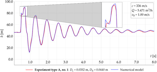
Figure 4.
Calculated and observed pressure oscillations during experiment no. 1.
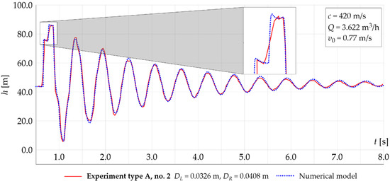
Figure 5.
Calculated and observed pressure oscillations during experiment no. 2.
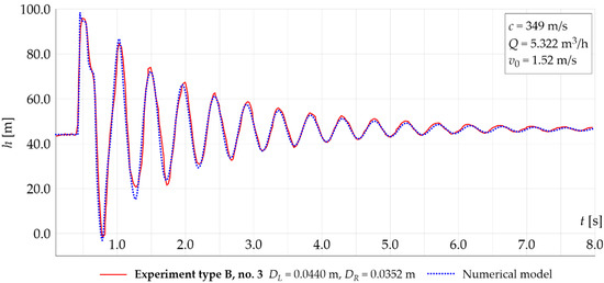
Figure 6.
Calculated and observed pressure oscillations during experiment no. 3.
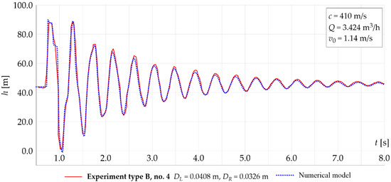
Figure 7.
Calculated and observed pressure oscillations during experiment no. 4.
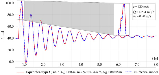
Figure 8.
Calculated and observed pressure oscillations during experiment no. 5.
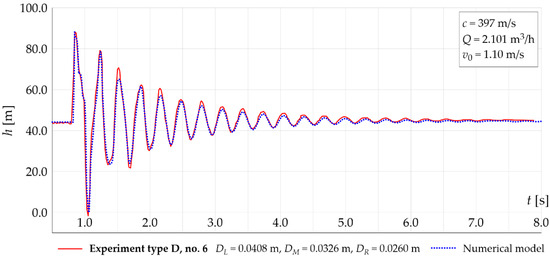
Figure 9.
Calculated and observed pressure oscillations during experiment no. 6.
Figure 4, Figure 5, Figure 6, Figure 7, Figure 8 and Figure 9 show that the pressure wave is strongly damped and time-dispersed. A particularly smooth h(t) function was recorded during experiments no. 1 and no. 3 (Figure 4 and Figure 6, respectively). For these tests, measurements were conducted using a pipe with a wall thickness of 2.4 mm (with an inner diameter of 35.2 mm) and a pipe with a wall thickness of 3.0 mm (with an inner diameter of 44 mm). For both of these tests (experiments no. 1 and no. 3), the ratio of the inside diameter to the wall thickness of the pipes was equal to D/s = 15. For other experiments (Table 1), the wall thickness to internal diameter ratio was constant and equalled D/s = 9. It is apparent from Figure 4 and Figure 6 that during the water hammer experiments in the pipeline system with thinner pipe walls, a stronger damping of the pressure wave can be observed. Additionally, it can be noticed that the values of the pressure wave velocity for pipes with thinner walls are lower compared to those for the rest of the experiments (Table 2). These lower values of the pressure wave velocity confirm a faster attenuation of disturbances in viscoelastic pipes with thinner walls.
In the hydraulic transient data (Figure 4, Figure 5, Figure 6, Figure 7, Figure 8 and Figure 9), additional disturbances typical of series-connected pipes are visible for the first pressure increase. The use of the MacCormack time-marching scheme along with the presented connection node equations satisfactorily reflects the pressure disturbances recorded during the measurements (zoom window in Figure 4 and Figure 5). It can be noted that the connection sequence of the pipes with various inner diameters has an influence on the pressure disturbance during the first pressure increase. In the case of the combination of tank–smaller-diameter-pipe–larger-diameter-pipe–outlet-valve (Figure 4 and Figure 5), the first pressure disturbance is not the maximum increase. This effect can also be observed for the water hammer test with three pipes in series (experiment no. 5). In the reverse configuration, the first recorded disturbance is also the maximum pressure increase (Figure 6, Figure 7 and Figure 9).
6. Conclusions
In the presented paper, the MacCormack explicit method was used to numerically solve transient flow equations in polymeric pipes. In order to take into account a sudden change in the pipeline diameter, the connection section boundary was used, which satisfies the head condition but takes into account two different values of the flow velocity on the left-hand side and the right-hand side of the connection node.
Including a term of retarded deformation in the continuity equation made it possible to take into account the viscoelastic behaviour of the pipe walls. The generalised one- and two-element Kelvin–Voigt model was used for numerical simulations. Despite including only a steady friction factor in the momentum equation, the calculated pressure fluctuations showed a satisfactory agreement with the laboratory data in terms of both phase and amplitude.
The use of the connection boundary condition made it possible to reproduce the pressure disturbances in the initial pressure increase related to the change in the diameter of the series-connected pipes.
Furthermore, a constant value of pressure wave velocity for the entire pipeline system was assumed. Further work needs to be performed to study water hammer in variable-property pipeline systems. Future studies will concentrate on simulating water hammer in serially connected pipes with various inner diameters and made of different materials. More broadly, research is also needed to address local losses during hydraulic transients due to diameter changes in pipeline systems.
Author Contributions
Conceptualisation, M.K. and A.M.; methodology, M.K., A.M. and A.K.; software, M.K.; validation, A.M., A.K., K.U. and M.S.; formal analysis, M.K., A.M. and K.U.; investigation, A.M. and A.K.; resources, A.M. and A.K.; data curation, M.K. and A.M.; writing—original draft preparation, M.K. and A.M.; writing—review and editing, A.K., K.U. and M.S.; visualisation, M.K.; supervision, M.K and A.M.; project administration, K.U. and M.S.; funding acquisition, M.K. and A.K. All authors have read and agreed to the published version of the manuscript.
Funding
This research received no external funding.
Institutional Review Board Statement
Not applicable.
Informed Consent Statement
Not applicable.
Data Availability Statement
The code generated during the study and experimental data are available from the corresponding author by request.
Conflicts of Interest
The authors declare no conflict of interest.
Nomenclature
| c | pressure wave velocity (m/s) |
| D | pipe internal diameter (m) |
| E0 | elastic bulk modulus of the spring (Pa) |
| Ek | elastic bulk modulus of the k-th Kelvin–Voigt element (Pa) |
| f | friction factor (-) |
| fs | Darcy‒Weisbach friction factor (-) |
| g | gravity acceleration (m/s2) |
| h | piezometric head (m) |
| J0 | instantaneous creep compliance (Pa−1) |
| Jk | creep compliance of the k-th Kelvin–Voigt element (Pa−1) |
| L | length of the individual pipe (m) |
| N | total number of Kelvin–Voigt elements (-) |
| Q | initial steady-state volumetric flow rate (m3/s) |
| p | pressure (Pa) |
| s | pipe wall thickness (m) |
| t | time (s) |
| v | average flow velocity (m/s) |
| v0 | initial average flow velocity (m/s) |
| vi,L | velocity on the left-hand side of the connection node (m/s) |
| vi,R | velocity on the right-hand side of the connection node (m/s) |
| x | space coordinate (m) |
| Δt | time step (s) |
| Δx | spatial step (m) |
| ƒ⊗0 | instantaneous (elastic) strain (-) |
| εr | retarded strain (-) |
| ƒ⊂k | viscosity of the k-th dashpot (kg/sm) |
| σ | stress (Pa) |
| τk | retardation time of the k-th Kelvin–Voigt element (s) |
| Acronyms | |
| HDPE | high-density polyethylene |
References
- Elleuch, R.; Taktak, W. Viscoelastic Behavior of HDPE Polymer Using Tensile and Compressive Loading. J. Mater. Eng. Perform. 2006, 15, 111–116. [Google Scholar] [CrossRef]
- Soares, A.K.; Covas, D.I.; Reis, L.F. Analysis of PVC Pipe-Wall Viscoelasticity during Water Hammer. J. Hydraul. Eng. 2008, 134, 1389–1394. [Google Scholar] [CrossRef]
- Bertaglia, G.; Ioriatti, M.; Valiani, A.; Dumbser, M.; Caleffi, V. Numerical Methods for Hydraulic Transients in Visco-Elastic Pipes. J. Fluids Struct. 2018, 81, 230–254. [Google Scholar] [CrossRef] [Green Version]
- Covas, D.; Stoianov, I.; Ramos, H.; Graham, N.; Maksimovic, C. The Dynamic Effect of Pipe-Wall Viscoelasticity in Hydraulic Transients. Part I—Experimental Analysis and Creep Characterization. J. Hydraul. Res. 2004, 42, 517–532. [Google Scholar] [CrossRef]
- Covas, D.; Stoianov, I.; Mano, J.F.; Ramos, H.; Graham, N.; Maksimovic, C. The Dynamic Effect of Pipe-Wall Viscoelasticity in Hydraulic Transients. Part II—Model Development, Calibration and Verification. J. Hydraul. Res. 2005, 43, 56–70. [Google Scholar] [CrossRef]
- Ferrante, M.; Massari, C.; Brunone, B.; Meniconi, S. Experimental Evidence of Hysteresis in the Head-Discharge Relationship for a Leak in a Polyethylene Pipe. J. Hydraul. Eng. 2011, 137, 775–780. [Google Scholar] [CrossRef]
- Duan, H.-F.; Ghidaoui, M.; Lee, P.J.; Tung, Y.-K. Unsteady Friction and Visco-Elasticity in Pipe Fluid Transients. J. Hydraul. Res. 2010, 48, 354–362. [Google Scholar] [CrossRef]
- Apollonio, C.; Covas, D.I.C.; de Marinis, G.; Leopardi, A.; Ramos, H.M. Creep Functions for Transients in HDPE Pipes. Urban Water J. 2014, 11, 160–166. [Google Scholar] [CrossRef]
- Pezzinga, G.; Brunone, B.; Cannizzaro, D.; Ferrante, M.; Meniconi, S.; Berni, A. Two-Dimensional Features of Viscoelastic Models of Pipe Transients. J. Hydraul. Eng. 2014, 140, 04014036. [Google Scholar] [CrossRef]
- Meniconi, S.; Brunone, B.; Ferrante, M. Water-Hammer Pressure Waves Interaction at Cross-Section Changes in Series in Viscoelastic Pipes. J. Fluids Struct. 2012, 33, 44–58. [Google Scholar] [CrossRef]
- Ferrante, M. Transients in a Series of Two Polymeric Pipes of Different Materials. J. Hydraul. Res. 2021, 1–10. [Google Scholar] [CrossRef]
- Malesinska, A.; Kubrak, M.; Rogulski, M.; Puntorieri, P.; Fiamma, V.; Barbaro, G. Water Hammer Simulation in a Steel Pipeline System with a Sudden Cross-Section Change. J. Fluids Eng. 2021. [Google Scholar] [CrossRef]
- Wylie, E.B.; Streeter, V.L.; Streeter, V.L. Fluid Transients; McGraw-Hill International Book Co.: New York, NY, USA, 1978; ISBN 978-0-07-072187-6. [Google Scholar]
- Chaudhry, M.H. Applied Hydraulic Transients, 3rd ed.; Springer: New York, NY, USA, 2014; ISBN 978-1-4614-8538-4. [Google Scholar]
- Keramat, A.; Tijsseling, A.S.; Hou, Q.; Ahmadi, A. Fluid–Structure Interaction with Pipe-Wall Viscoelasticity during Water Hammer. J. Fluids Struct. 2012, 28, 434–455. [Google Scholar] [CrossRef] [Green Version]
- Covas, D.; Stoianov, I.; Ramos, H.; Graham, N.; Maksimović, Č.; Butler, D. Water Hammer in Pressurized Polyethylene Pipes: Conceptual Model and Experimental Analysis. Urban Water J. 2004, 1, 177–197. [Google Scholar] [CrossRef]
- Weinerowska-Bords, K. Viscoelastic Model of Waterhammer in Single Pipeline—Problems and Questions. Arch. Hydro-Eng. Environ. Mech. 2006, 53, 331–351. [Google Scholar]
- Adamkowski, A.; Lewandowski, M. Experimental Examination of Unsteady Friction Models for Transient Pipe Flow Simulation. J. Fluids Eng. 2006, 128, 1351–1363. [Google Scholar] [CrossRef]
- Bergant, A.; Ross Simpson, A.; Vìtkovsky, J. Developments in Unsteady Pipe Flow Friction Modelling. J. Hydraul. Res. 2001, 39, 249–257. [Google Scholar] [CrossRef] [Green Version]
- MacCormack, R. The Effect of Viscosity in Hypervelocity Impact Cratering. In Proceedings of the 4th Aerodynamic Testing Conference, Cincinnati, OH, USA, 28 April 1969. [Google Scholar]
- MacCormack, R. A Numerical Method for Solving the Equations of Compressible Viscous Flow. In Proceedings of the 19th Aerospace Sciences Meeting, American Institute of Aeronautics and Astronautics, St. Louis, MO, USA, 12 January 1981. [Google Scholar]
- Ngondiep, E.; Kerdid, N.; Abdulaziz Mohammed Abaoud, M.; Abdulaziz Ibrahim Aldayel, I. A Three-level Time-split MacCormack Method for Two-dimensional Nonlinear Reaction-diffusion Equations. Int. J. Numer. Methods Fluids 2020, 92, 1681–1706. [Google Scholar] [CrossRef]
- Wan, W.; Huang, W. Water Hammer Simulation of a Series Pipe System Using the MacCormack Time Marching Scheme. Acta Mech. 2018, 229, 3143–3160. [Google Scholar] [CrossRef]
- Wan, W.; Zhang, B.; Chen, X.; Lian, J. Water Hammer Control Analysis of an Intelligent Surge Tank with Spring Self-Adaptive Auxiliary Control System. Energies 2019, 12, 2527. [Google Scholar] [CrossRef] [Green Version]
- Weinerowska-Bords, K. Alternative Approach to Convolution Term of Viscoelasticity in Equations of Unsteady Pipe Flow. J. Fluids Eng. 2015, 137, 054501. [Google Scholar] [CrossRef]
- Ferrante, M.; Capponi, C. Calibration of Viscoelastic Parameters by Means of Transients in a Branched Water Pipeline System. Urban Water J. 2018, 15, 9–15. [Google Scholar] [CrossRef]
- Choura, O.; Capponi, C.; Meniconi, S.; Elaoud, S.; Brunone, B. A Nelder–Mead Algorithm-Based Inverse Transient Analysis for Leak Detection and Sizing in a Single Pipe. Water Supply 2021, ws2021030. [Google Scholar] [CrossRef]
Publisher’s Note: MDPI stays neutral with regard to jurisdictional claims in published maps and institutional affiliations. |
© 2021 by the authors. Licensee MDPI, Basel, Switzerland. This article is an open access article distributed under the terms and conditions of the Creative Commons Attribution (CC BY) license (https://creativecommons.org/licenses/by/4.0/).