Exhaustive Comparison between Linear and Nonlinear Approaches for Grid-Side Control of Wind Energy Conversion Systems

Abstract

In this paper, we propose a comparative study of linear and nonlinear algorithms designed for grid-side control of the power flow in a wind energy conversion system. We performed several simulations and experiments with step and variable power scenarios for different values of the DC-link capacity with the DC storage element being the key element of the grid-side converter. The linear control was designed on the basis of the internal model control theory where an active damping was added to avoid steady state errors. Nonlinear controls were built using first and second order sliding mode controls with theoretical considerations to ensure accuracy and stability. We observed that the first order sliding mode control was the most efficient algorithm for controlling the DC-link voltage but that the chattering degraded the quality of the energy injected into the grid as well as the efficiency of the grid-side converter. The linear control caused overshoots on the DC-link voltage; however, this algorithm had better performance on the grid side due to its smoother control. Finally, the second order sliding mode control did not prove to be more robust than the other two algorithms. This can be explained by the fact that this control is theoretically more sensitive to converter losses.

1. Introduction

Electricity generation from wind energy has developed rapidly in recent years and will continue to grow in the next decade [1,2,3,4,5,6]. The main issue for this technology relies on the high variability of the source power, which requires designing a sophisticated Wind Energy Conversion System (WECS) [7,8,9]. Different kinds of electric generators are used in WECSs; however, Permanent Magnet Synchronous Generators (PMSG) are becoming increasingly common [10,11]. A WECS using a PMSG is generally divided into two parts, the generator-side system and the grid-side system connected to each other by a DC-link capacity. Systems without DC energy storage can also be designed using matrix converters [12,13,14]; however, these are still not widespread.

The objective of the generator-side control is to capture the maximum power from wind—whatever its velocity—while the objective of the grid-side control is to control the active and reactive power flow between the WECS and the grid [15,16,17,18]. Both parts of the WCES can be designed separately since they are decoupled by the DC-link capacity. In this study, we focus our attention on the grid side control; only the high variability of the collected power by the generator-side system will be considered here. The grid-side control is often performed in a grid-voltage synchronous reference frame $\left(d,q\right)$—the so-called voltage oriented control (VOC) [19].

In this approach, the projection of the grid currents into d and q-axis allows the control of active and reactive powers separately. The controller is generally constituted by two cascaded loops: an inner current loop to regulate the grid current and an outer voltage loop designed for balancing the power flow. While the internal loop for regulating currents can be designed using traditional linear controllers, the external loop for regulating the DC-link voltage is more problematic: the power conservation law leads a priori to a nonlinear problem. Recently, different methods have been proposed to solve this nonlinear problem using Sliding Mode Controls (SMC) of first or second orders with theoretical considerations [20,21] or more empirical approaches using, for example, fuzzy logic [22,23] or neural networks [24,25].

In recent years, SMC has been widely used in the control of non-linear systems and systems with uncertain parameters, namely: electric motor, robotics, and power converters [26,27,28]. The main advantage of this approach is the nature of its command, which alters the nonlinear dynamics of the controlled system and ensures its stability and robustness to uncertainties and disturbances affecting the system [29]. The First Order Sliding Mode Control (SMC1) [30,31], is one of the most used techniques in the control of linear systems with uncertain parameters, and non-linear systems that can be well modeled by a linear system, around the operating point. The second order sliding mode control (SMC2) [32,33,34], is sometimes preferred to as SMC1, because the nature of this control considerably attenuates the chattering phenomenon generated by SMC1. SMC2 also guarantees a convergence in a finite time as well as maintenance of the zero control error [35].

The numerical and experimental results prove that the proposed methods make it possible to control the DC-link voltage successfully. A comparison with traditional PI controllers—where the nonlinear nature of the problem is not addressed—has been proposed; however, these comparative studies are not completely convincing as the degrees of freedom in the choice of parameters were not discussed. In addition, while the side generator control is inevitably a nonlinear problem [36,37], a feedback linearization is possible to rigorously deal with the grid-side control using the internal control model theory [38,39]. This linear solution is not considered as an alternative in the previous mentioned works even though it offers better performance over empirically designed PI controllers.

In the literature, most of the research studied the robustness of control algorithms in the event of a fault in the system [40]. However, the performance of the grid-side control is largely related to the capacity of the DC-link, which acts as a buffer. The robustness of the algorithms must, therefore, also be characterized according to the value of the DC-link capacity, including in the absence of fault in the systems. However, as large values of the DC-link capacity are generally used, it is almost impossible to objectively assess the performance of one algorithm over the other ones.

The main objective of this paper is to provide an accurate comparison of the performance and robustness between linear and non-linear approaches in the grid side control when there is no fault in the system. This study was based on simulations and on an experimental bench that reproduced the behavior of a WECS. To assess the robustness of the different strategies, scenarios with different values of the DC-link capacity were performed, the DC energy storage being the key element in the grid-side converter. Only algorithms with a theoretical basis were studied, since only these approaches make it possible to set the value of the algorithm parameters according to the value of the DC-link capacity. Our methodology consisted in calibrating the parameters of the different algorithms so that the performances were the same for the greatest value of the DC link capacity in the case of step power.

Then, the performances were evaluated for different values of the DC link capacity, where the value of the parameters for the different algorithms were adjusted according to the value of the capacity. In Section 2, the structure of the grid-side converter is presented as well as the equations that govern the dynamics for the line currents and the DC-link voltage. In Section 3, the theoretical developments for the regulation of the DC-link capacity voltage are detailed for the linear and nonlinear controls. The numerical and experimental results are reported in Section 4 and Section 5, respectively, where the error on the DC-link voltage, the quality of the line current and the efficiency of the grid-side system are compared between the algorithms for different values of the DC-link capacity in the case of step power and variable powers.

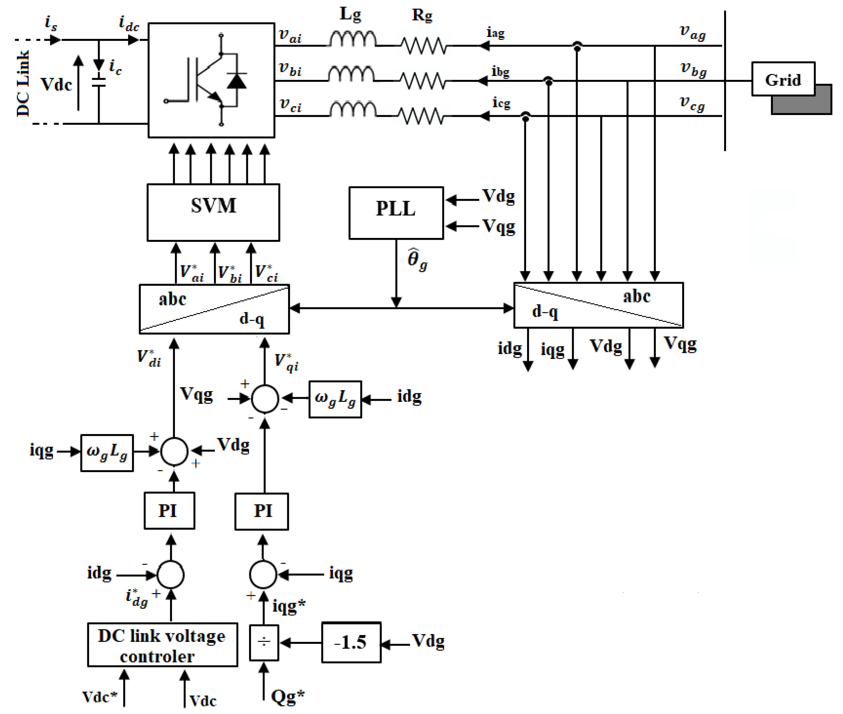
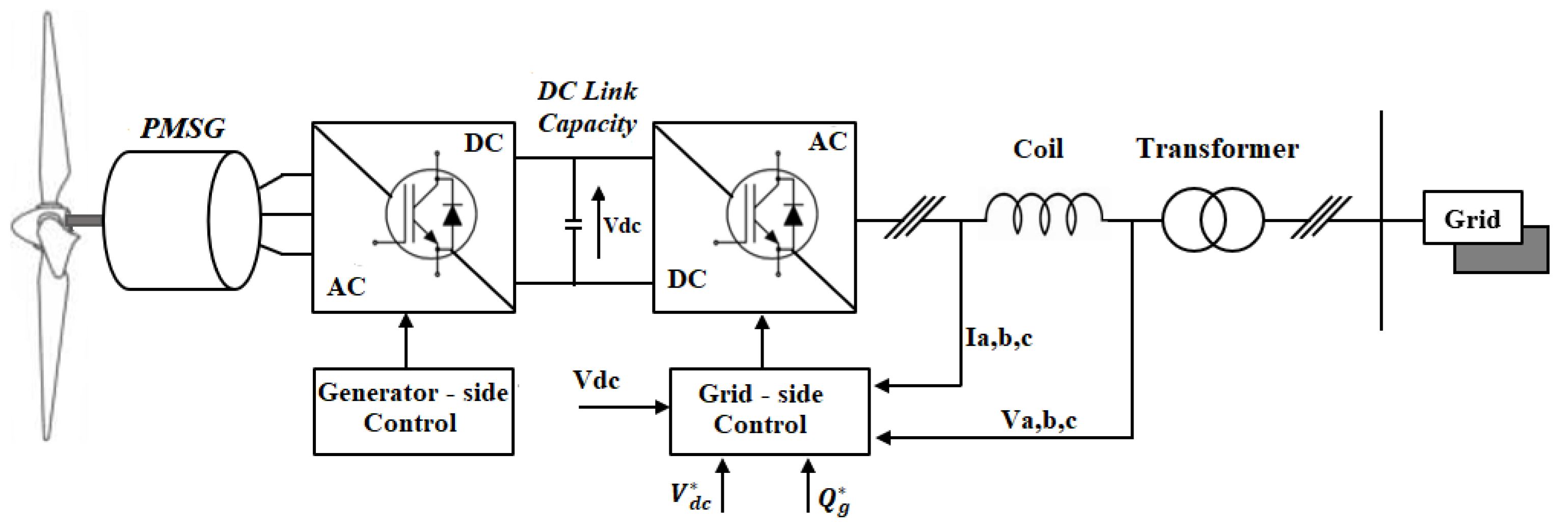
2. Grid-Side Conversion System

The structure of the WECS is shown in Figure 1: the grid-side converter is composed of a DC-link capacitor, a two-level voltage source inverter, a choke coil, and a transformer. The power flow between the DC-link capacitor and the grid is bidirectional: the power generated by WECS is naturally injected to the grid, and the system can also provide a part of reactive power as required by the grid operator.

The power flow through the inverter is controlled by a VOC as illustrated in Figure 2. The algorithm is implemented in the grid-voltage synchronous reference frame $\left(d,q\right)$, where all the variables are DC components in a steady state. In particular, the active power $P_g$ and reactive power $Q_g$ for the grid-side can be calculated using the following equation:

$$\left\{\begin{array}{cc}{P}_g=\hfill & \frac{3}{2}\left(V_{dg}{i}_{dg}+V_{qg}{i}_{qg}\right)\hfill \\ \hfill & \\ Q_g=\hfill & \frac{3}{2}\left(V_{qg}{i}_{dg}-V_{dg}{i}_{qg}\right)\hfill \end{array}\right.$$

(1)

where $i_{dg}$ and $i_{qg}$ (respectively, $V_{dg}$ and $V_{qg}$) are the d-axis and q-axis components of the line currents (the grid voltages).

The d-axis of the synchronous frame is chosen to be aligned with the grid voltage vector. Therefore, the d-axis grid voltage is equal to its magnitude ($V_{dg}=V_g$), and the resultant q-axis voltage $V_{qg}$ is equal to zero. This operation is realized using a Phase Locked Loop (PLL) [41]. In these conditions, Equation (1) is simplified as:

$$\left\{\begin{array}{cc}{P}_g=\hfill & \frac{3}{2}{V}_g{i}_{dg}\hfill \\ \hfill & \\ Q_g=\hfill & -\frac{3}{2}{V}_g{i}_{qg}\hfill \end{array}\right.$$

(2)

According to Equation (2), active and reactive powers depend on the d-axis and q-axis currents, respectively. Thus, the control of powers can be carried out from reference values of the currents $i_{dg}^{*}$ and $i_{qg}^{*}$. This leads to the required voltage $V_{di}^{*}$ and $V_{qi}^{*}$ at the output of the inverter (see Figure 2), which, in turn, results in gate pulses for the inverter switches performed using a space vector modulation (SVM). The dynamics to consider in the controller design rely on the voltage drop between the inverter and the grid:

$$\left\{\begin{array}{cc}{V}_{di}=\hfill & V_g-\left[R_g{i}_{dg}+L_g\frac{d{i}_{dg}}{dt}-{\omega }_g{L}_g{i}_{qg}\right]\hfill \\ \hfill & \\ V_{qi}=\hfill & -\left[R_g{i}_{qg}+L_g\frac{d{i}_{qg}}{dt}+{\omega }_g{L}_g{i}_{dg}\right]\hfill \end{array}\right.$$

(3)

with ${\omega }_g$ is the grid angular frequency, and the choke coil is modeled by an inductance $L_g$ and a resistance $R_g$ in series.

Equation (3) shows that the system is linear with respect to $i_{dg}$ and $i_{qg}$ but cross-coupled. This configuration may lead to difficulties in designing the PI controller and unsatisfactory dynamic performance. To avoid this issue, a decoupling is performed dealing with the terms ${\omega }_g{L}_g{i}_{qg}$ and ${\omega }_g{L}_g{i}_{dg}$ (see Figure 2). The parameters of the PI controller for the currents $i_{dg}$ and $i_{qg}$ can then be calculated in order to achieve a first order closed-loop with a time constant ${\tau }_i$.

Considering a given reference reactive power $Q_g^{*}$, the reference q-axis current $i_{qg}^{*}$ can be obtained from Equation (2):

$$i_{qg}^{*}=-\frac{2Q_g^{*}}{3V_g}$$

(4)

Instead of setting the reference current $i_{qg}^{*}$ according to Equation (4), a traditional PI controller could be implemented to address the uncertainties of the model.

The reference d-axis current $i_{dg}^{*}$, which is related to the active power of the system, is generated by the DC-link voltage control. When the inverter operates in a steady state, the DC-link voltage of the inverter must be kept to a constant reference value $V_{dc}^{*}$ in order to properly realize the power transfer. The dynamic of $V_{dc}$ can be derived from power considerations. Assuming an ideal inverter without losses, the variation of the stored energy in the DC-link capacity is such that:

$$C{V}_{dc}\frac{d{V}_{dc}}{dt}=P_s-P_g=V_{dc}{i}_s-\frac{3}{2}{V}_g{i}_{dg}$$

(5)

where $P_s$ is the power delivered by the generator-side system and $i_s$ is the current flowing from the generator-side system to the DC-link capacity.

Equation (5) is nonlinear with respect to $V_{dc}$. Therefore, the control of the DC-link voltage should not be realized correctly with conventional PI controllers. To address this issue, two different strategies are proposed in the next section. In Section 3.1, a new variable $W={V_{dc}}^2$ is introduced and Equation (5) is linearized considering the power $P_s$ as a perturbation, which enables the design of a linear controller; active damping is, however, necessary in order to properly set the properties of the closed-loop. In Section 3.2 and Section 3.3, the nonlinear problem is directly solved using first and second order sliding mode controls, techniques that are particularly suitable to deal with nonlinear problems.

3. Control Strategies of the DC-Link Voltage

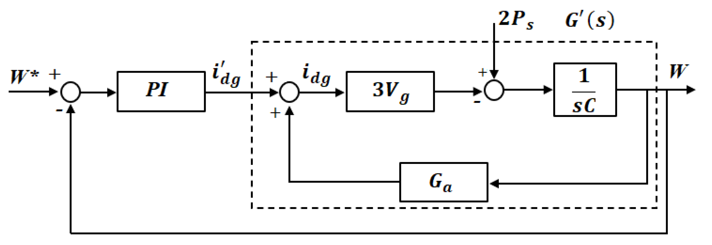
3.1. Linear Control with Active Damping

The design of voltage controller using a traditional PI is possible due to feedback linearization. Introducing the variable $W={V_{dc}}^2$ in Equation (5), one finds:

$$\frac{1}{2}C\frac{dW}{dt}=P_s-\frac{3}{2}{V}_g{i}_{dg}=\sqrt{W}{i}_s-\frac{3}{2}{V}_g{i}_{dg}$$

(6)

The error e in the DC-link control is then defined according to the variable W:

$$e=W^{*}-W$$

(7)

where $W^{*}={V_{dc}^{*}}^2$.

Equation (6) is linear with respect to W only if $P_s$ is considered as an unknown perturbation. In these conditions, linear theory can be applied and the opened-loop transfer function G defined when the perturbation $P_s$ is set to zero is given by

$$G\left(s\right)=\frac{\mathrm{L}\left[W\right]\left(s\right)}{\mathrm{L}\left[i_{dg}\right]\left(s\right)}=-\frac{3V_g}{Cs}$$

(8)

where $\mathrm{L}\left[u\right]\left(s\right)$ is the Laplace transform of the time function $u\left(t\right)$.

Using a proportional corrector, the closed-loop transfer function would be of the first order making it possible to adjust the time response for $V_{dc}$. However, this choice introduces a steady state error e when a constant perturbation $P_s$ is considered. An alternative consists in adding an active damping as shown in Figure 3 [38]. The basic idea is to introduce a damping term $G_a$ to modify the transfer function G. An interpretation is that $G_a$ induces a fictitious resistive effect in addition to the capacitive real one; thus, the corrected current $i_{dg}^{\prime }$ is such that:

$$i_{dg}^{\prime }=i_{dg}-G_{a}W$$

(9)

The corrected opened-loop transfer function $G^{\prime }$ defined when the perturbation $P_s$ is set to zero is given by:

$$G^{\prime }\left(s\right)=\frac{\mathrm{L}\left[W\right]\left(s\right)}{\mathrm{L}\left[i_{dg}^{\prime }\right]\left(s\right)}=\frac{3V_g}{3V_g{G}_a+Cs}$$

(10)

Using a PI corrector with the proper parameters $k_p$ and $k_i$, the closed-loop transfer function will be of the first order; interestingly, no steady state error e will be expected when a constant perturbation $P_s$ is considered.

Thus, the command $i_{dg}^{*}$ reads

$$\begin{array}{cc}{i}_{dg}^{*}\hfill & =k_{p}e+k_i\int e+G_{a}W\hfill \end{array}$$

(11)

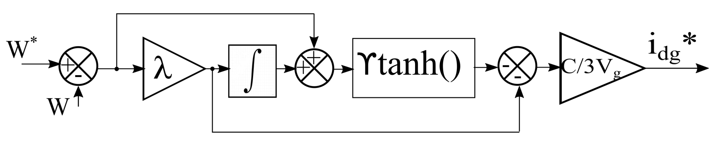
3.2. First Order Sliding Mode Control (SMC1)

Sliding mode control algorithms ensure zero tracking error through the sliding variable and its first-time derivative in time. Depending on the choice of the sliding variable, it can be theoretically guaranteed that the controller will have attractive properties, particularly with regard to the stability [42].

From Equation (7), the DC-link tracking error has the following dynamic:

$$\dot{e}=\dot{W^{*}}-\dot{W}$$

(12)

Using Equation (6), one finds:

$$\dot{e}=\dot{W^{*}}-\frac{2}{C}\left(P_s-\frac{3}{2}{V}_g{i}_{dg}\right)$$

(13)

When the DC-link reference voltage is constant ($\dot{W^{*}}=0$), the previous equation is simplified to

$$\dot{e}=-\frac{2}{C}{P}_s+\frac{3}{C}{V}_g{i}_{dg}=-\frac{2}{C}\sqrt{W}{i}_s+\frac{3}{C}{V}_g{i}_{dg}$$

(14)

In the case of SMC1, the sliding variable S is chosen such that

$$\dot{S}=\dot{e}+\lambda e$$

(15)

where $\lambda >0$ is a parameter to adjust the speed of the control. The authors in [20] proposed a SMC1 based on the error term $V_{dc}^{*}-V_{dc}$ instead of e defined in Equation (7). In this paper, we preferred maintaining the same formalism used for the design of the linear controller.

The strategy of SMC1 is governed by the following dynamics:

$$\dot{S}=d-\gamma sign\left(S\right)$$

(16)

where d is the perturbation related to $P_s$ in a similar way as in the design of the linear controller in Section 3.1. Setting $\gamma$ such that $\gamma >\left|d\right|$, the system is proven to be asymptotically stable [20]. Combining Equations (15) and (16), one finds:

$$\dot{e}=d-\gamma sign\left(S\right)-\lambda e$$

(17)

Identifying Equations (14) and (17), one obtains that the perturbation is $d=-2P_s/C$ and the command $i_{dg}^{*}$ such that

$$i_{dg}^{*}=\frac{C}{3V_g}\left(-\lambda e-\gamma sign\left(e+\lambda \int e\right)\right)$$

(18)

The discontinuity in Equation (18) generates chattering of the command. To avoid this issue, the sign function in Equation (18) is generally changed to a smoother function: the authors in [20] proposed using function $tanh\left(\xi S\right)$, where $\xi$ is chosen to moderate the effect of the chattering phenomenon as shown in Figure 4.

The corrected command reads:

$$i_{dg}^{*}=\frac{C}{3V_g}\left(-\lambda e-\gamma tanh\left[\xi \left(e+\lambda \int e\right)\right]\right)$$

(19)

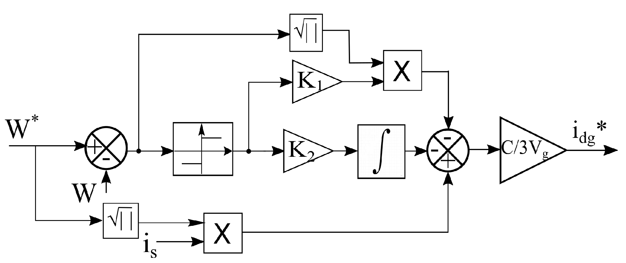
3.3. Second Order Sliding Mode Control (SMC2)

SMC2 is generally presented as a solution to overcome the chattering phenomenon. In [21], a SMC2 was proposed using the error term $V_{dc}^{*}-V_{dc}$ instead of e defined in Equation (7). In this paper, we preferred to maintain the same formalism used for the design of the linear controller. This choice simplifies the derivation of the command as shown in this section. Equation (14) can be rewritten as

$$\dot{e}=\frac{3}{C}{V}_g{i}_{dg}-\frac{2}{C}\sqrt{W^{*}}{i}_s+\frac{2}{C}\left(\sqrt{W^{*}}-\sqrt{W}\right)i_s$$

(20)

From Equation (20), the control term u and the perturbation term d are chosen such that

$$\begin{array}{cc}\hfill & \dot{e}=u+d\\ \hfill & \\ \mathrm{where}\hfill & \left\{\begin{array}{cc}u=\hfill & \frac{3}{C}{V}_g{i}_{dg}-\frac{2}{C}\sqrt{W^{*}}{i}_s\hfill \\ \hfill & \\ d=\hfill & \frac{2}{C}\left(\sqrt{W^{*}}-\sqrt{W}\right)i_s\hfill \end{array}\right.\end{array}$$

(21)

The strategy of the SMC2 control is governed by the following dynamics:

$$\left\{\begin{array}{cc}u=\hfill & -k_1\sqrt{\left|e\right|}sign\left(e\right)+\omega \hfill \\ \hfill & \\ \dot{\omega }=\hfill & -k_{2}sign\left(e\right)\hfill \end{array}\right.$$

(22)

Identifying Equations (21) and (22), one obtains that the command $i_{dg}^{*}$ is such that:

$$i_{dg}^{*}=\frac{C}{3V_g}\left(-k_1\sqrt{\left|e\right|}sign\left(e\right)-k_2\int sign\left(e\right)+\frac{2}{C}\sqrt{W^{*}}{i}_s\right)$$

(23)

Figure 5 illustrate the block diagram of SMC2.

To guarantee the asymptotic stability [43], the following condition is required on the perturbation term d:

$$\left|d\right|\le \delta \sqrt{\left|e\right|}$$

(24)

where the constant $\delta$ defines a bound for the perturbation term. From Equation (21), the value of $\delta$ can be set as the following:

$$\delta =\frac{2}{C}\sqrt{\frac{\Delta v_{dcmax}}{2-\Delta v_{dcmax}}}{i}_{smax}$$

(25)

where $\Delta v_{dcmax}$ is the maximum relative error on the DC-link voltage and $i_{smax}$ is the maximum current produced by the WECS.

Specific conditions on the gains $k_1$ and $k_2$ can then be established with respect to $\delta$ in order to ensure robustness to uncertainties and stability:

$$\left\{\begin{array}{cc}{k}_1>\hfill & 2\delta \hfill \\ k_2>\hfill & {\displaystyle k_1\frac{\frac{5}{2}{k}_1\delta +2{\delta }^2}{k_1-2\delta }}\hfill \end{array}\right.$$

(26)

The command $i_{dg}^{*}$ in SMC2 depends on the current $i_s$, which is a serious drawback compared to the linear controller or SMC1. This choice is motivated by the theoretical condition (24), which requires that the perturbation d decreases to zero similarly to the root mean square of e.

4. Simulation Results

To compare these algorithms, simulations were performed using Matlab/Simulink. Since the core of the problem deals with the grid-side converter and the performance between the algorithms presented in Section 3, the generator-side was reduced to a perfect generator. The grid side conversion system was modeled more finely using the parameters reported in

Table 1. Common electric and control parameters for the grid side converter in all simulations and experiments.

Electric Parameter	Value
Reference DC link voltage $V_{dc}^{*}$	$400$V
Grid side voltage $V_g$	$100$V
Grid side frequency ${\omega }_g/\left(2\pi \right)$	$50$Hz
Coil Resistance $R_g$	$0.37\mathsf{\Omega }$
Coil Inductance $L_g$	$50$mH
Control Parameter	Value
Proportional gain to control $\{i_{dg},i_{qg}\}$	$246.7$
Integral gain to control $\{i_{dg},i_{qg}\}$	$33.3$
Time constant ${\tau }_i$ to control $\{i_{dg},i_{qg}\}$	$1.5$ms

, which are consistent with the experimental bench described in Section 5. For different DC-link capacity values ranging from $6\mathsf{\mu }$F to $120\mathsf{\mu }$F, the performance of the different algorithms was compared based on the quality of the DC-link voltage control and of the current injected on the grid.

The DC-link capacity is the key element in the grid side converter: the higher this is, the better the converter will support the power flow. Another possibility to test the different algorithms would have been to set the value of the DC-link capacity and to perform scenarios where the power injected varied over a large range. However, under these conditions, the defects of the other elements in the system would have had a significant influence, in particular the inverter whose losses and voltage drops are related to the flowing currents. This is why we preferred to carry out the experiments with scenarios where the order of magnitude of the powers remained the same and where the performances between algorithms were evaluated for different values of the DC-link capacity.

The common electric and control parameters in all simulations and experiments are reported in Table 1.

Two different types of scenarios were performed. In the first scenario, a step of the power supplied by the system on the generator side was considered as well as a step of the reactive power required. In the second scenario, a more realistic configuration was tested where the variability of the power injected by a WECS into the grid was modeled.

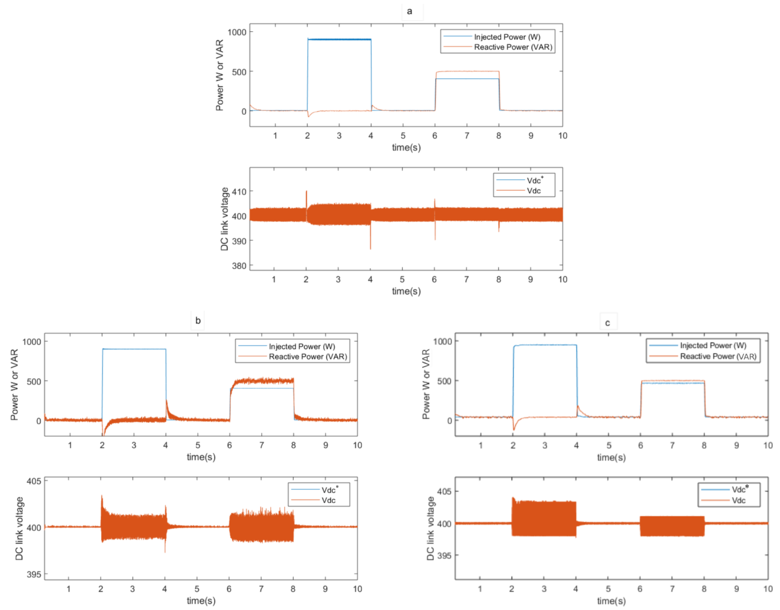
4.1. Results with Step Power

In this scenario, no power was injected at the beginning; then, suddenly, 900 W was injected for 2 s; and later, 400 W was injected and, at the same time, a reactive power $Q_g^{*}$ of 500 VAR was required for 2 s. Figure 6 shows the simulation results for the three algorithms described in Section 3 with a value for the DC-link capacity of $30\mathsf{\mu }$F.

As shown in Table 1, the DC-link reference voltage was set to $400$V. Figure 6a shows that, at the moment where power was injected, the real voltage $V_{dc}$ presented a jump that was quickly attenuated, which was expected for the designed linear controller in the presence of a perturbation step. After this transient effect, it can be seen that the voltage $V_{dc}$ was maintained around 400 V with a kind of noise around the reference value. In order to quantify the two phenomena described above, two indicators ${ϵ}_{max}$ and ${ϵ}_{RMS}$ were introduced. They measured the error on the DC-link voltage using the maximum norm and L2-norm:

$${ϵ}_{max}=\underset{t\in T}{max}|V_{dc}^{*}\left(t\right)-V_{dc}\left(t\right)|$$

(27)

$${ϵ}_{RMS}=\sqrt{\frac{1}{T}{\int }_T{(V_{dc}^{*}\left(t\right)-V_{dc}\left(t\right))}^{2}dt}$$

(28)

where two different periods of time T were considered: the first one when only active power is injected ($P_g>0$ and $Q_g=0$) and the second one when both active power is injected and reactive power is required ($P_g>0$ and $Q_g>0$).

The values of ${ϵ}_{max}$ and ${ϵ}_{RMS}$ for a given scenario depend on the choice of the algorithm parameters. In order to make a comparative study of the control strategies presented in Section 3, we sought to adjust the parameters of the linear controller and the nonlinear controllers SMC1 and SMC2 so that the errors ${ϵ}_{max}$ and ${ϵ}_{RMS}$ were approximately the same for a capacity value of $120\mathsf{\mu }$F.

Concerning the linear control, we define the parameter ${\tau }_v$ related the time response of the closed-loop in Figure 3; ${\tau }_v$ is also chosen for the time response of the transfer function $G^{\prime }\left(s\right)$. The value of ${\tau }_v$ is required to be equal or greater than ${\tau }_i$ since ${\tau }_i$ is related to the time response of the inner loops for the line currents control (see Figure 2). Then, the value for the parameters of the PI controller with active damping are computed as following:

$$\left\{\begin{array}{c}{G}_a=C/\left(3\sqrt{2}{V}_g{\tau }_v\right)\hfill \\ k_p=-G_a\hfill \\ k_i=-G_a/{\tau }_v\hfill \end{array}\right.$$

(29)

where ${\tau }_v=1.5$ms in all experiments.

Concerning the SMC1 controller, the parameter $\lambda$ is related to the inverse of the time constant in the exponential decrease of error e when the solution remains on the sliding surface $S=0$ (see Equation (15) with $\dot{S}=0$). The parameter $\gamma$ must meet the condition $\gamma >\left|d\right|=2P_s/C$. In order to obtain similar values of ${ϵ}_{max}$ and ${ϵ}_{RMS}$ as with the linear control when $C=120\mathsf{\mu }$F, the parameters of the SMC1 controller were adjusted as follows:

$$\left\{\begin{array}{c}\lambda =1/\left(5{\tau }_v\right)\hfill \\ \gamma =2\times P_{smax}/C\hfill \end{array}\right.$$

(30)

where $P_{smax}=1600W$. In addition, $\xi$ was set to ${10}^{-4}$ because a better control was observed.

Concerning the SMC2 controller, the value of $\delta$ was computed by Equation (25) with the maximum relative error on the DC link voltage $\Delta v_{dcmax}=5/400$ (which results in a maximum overshoot of 5 V) and the maximum current produced by the WECS $i_{smax}=4$A (which results in a maximum injected power of $1600$W when $V_{dc}=400$V). In order to obtain similar values of ${ϵ}_{max}$ and ${ϵ}_{RMS}$ as with the linear control when $C=120\mathsf{\mu }$F in one hand and to satisfy the required conditions set in Equation (26) on the other hand, the parameters of the SMC2 controller were adjusted as follows:

$$\left\{\begin{array}{c}{k}_1=6.3\delta \hfill \\ k_2=26.9{\delta }^2\hfill \end{array}\right.$$

(31)

where $\delta =\frac{2}{C}\sqrt{\frac{5/400}{2-5/400}}\times 4$

For each value of the DC-link capacity C, the scenario of power injection illustrated in Figure 6 was carried out. The parameters of the different controllers were computed with respect of the value of the DC-link capacity according to Equation (29) for the linear controller, Equation (30) for SMC1 and Equation (31) for SMC2. We postulate that this approach is suitable to compare the performances of the different algorithms for the control of the DC-link voltage. Indeed, the other elements of the conversion chain, the inverter and the choke coil, remain the same and are subjected to currents and voltages of the same order of magnitude in the different simulations and experiments.

Table 2. Comparison of the errors, ${ϵ}_{max}$ and ${ϵ}_{RMS}$, and the THD line current obtained by the three algorithms in the case of step power.

Indicators	C	Step Power
		$\mathit{P}>0$ and $\mathit{Q}=0$			$\mathit{P}>0$ and $\mathit{Q}>0$
		Linear Control	SMC1	SMC2	Linear Control	SMC1	SMC2
${ϵ}_{max}$	$6\mathsf{\mu }$F	$41.5$	$8.9$	12	$39.6$	$4.8$	13
	$12\mathsf{\mu }$F	$20.6$	$5.6$	$7.1$	$19.4$	$2.9$	$7.2$
	$30\mathsf{\mu }$F	$12.2$	$3.9$	$4.8$	$9.9$	$2.2$	$2.6$
	$60\mathsf{\mu }$F	$5.2$	$2.8$	$2.5$	$4.4$	$1.4$	$1.9$
	$120\mathsf{\mu }$F	$2.9$	$2.3$	$1.2$	$2.4$	$1.3$	$0.8$
${ϵ}_{RMS}$	$6\mathsf{\mu }$F	$7.9$	$0.3$	$0.6$	$3.9$	$0.4$	$0.7$
	$12\mathsf{\mu }$F	3	$0.2$	$0.3$	$1.9$	$0.3$	$0.4$
	$30\mathsf{\mu }$F	1	$0.1$	$0.2$	$0.6$	$0.2$	$0.1$
	$60\mathsf{\mu }$F	$0.5$	$0.2$	$0.2$	$0.3$	$0.2$	$0.1$
	$120\mathsf{\mu }$F	$0.2$	$0.1$	$0.2$	$0.1$	$0.2$	$0.1$
THD (%)	$6\mathsf{\mu }$F	$3.3$	$4.4$	$3.9$	$3.7$	$3.9$	$2.1$
	$12\mathsf{\mu }$F	$2.4$	$4.4$	$3.8$	$2.9$	$2.9$	$1.6$
	$30\mathsf{\mu }$F	$2.1$	$4.7$	$3.9$	$2.6$	$2.6$	$1.5$
	$60\mathsf{\mu }$F	$1.9$	$4.7$	$4.2$	$2.4$	$3.3$	$1.7$
	$120\mathsf{\mu }$F	$1.9$	$4.9$	$4.5$	$2.4$	4	$1.9$

illustrates a comparison between the ${ϵ}_{max}$, ${ϵ}_{RMS}$ and the THD line current indicators obtained by the three algorithms in the case of step power: where only active power is injected ($P_g=900$ W and $Q_g=0$) and where the active power is injected and the reactive power is required ($P_g=400$ W and $Q_g=500$ VAR).

In the case where only the active power is injected, we can see that ${ϵ}_{max}$ and ${ϵ}_{RMS}$ for linear control increased when the value of the capacity decreased, reaching $41.5$ V for ${ϵ}_{max}$ and $7.9$ V for ${ϵ}_{RMS}$ when $C=6\mathsf{\mu }$F. In the opposite case, for non-linear controllers (SMC1 and SMC2) the dynamic depended less on the value of the capacity: in the case of SMC1, we observed that there was no great effect when the value of the capacity decreased, with a maximum error ${ϵ}_{max}=8.9$ V and ${ϵ}_{RMS}=0.3$ V when $C=6\mathsf{\mu }$F. This remained almost the same for the case of SMC2, with a maximum error ${ϵ}_{max}=12$ V and ${ϵ}_{RMS}=0.6$ V when $C=6\mathsf{\mu }$F.

In addition, we observed that all the strategies had tolerable THD values for injection; however, the linear control proved its efficiency with a THD of around $2.3\%$. In contrast, the THD rates for SMC1 and SMC2 remained around $4.6\%$ and $4.2\%$, respectively.

In the case where reactive power was requested ($P_g=400$ W and $Q_g=500$ VAR), we observed that the controllers reacted in the same way as in the case where only active power was injected, except that, in this scenario, the errors ${ϵ}_{max}$ and ${ϵ}_{RMS}$ were reduced, as the injected power was only 400 W.

We also noticed that the THD rate for the current di not have a significant change for all strategies. However, the simulation results generally showed that the reactive power control was performed independently and had no effect on the control of the $V_{dc}$ voltage and the quality of the injected current.

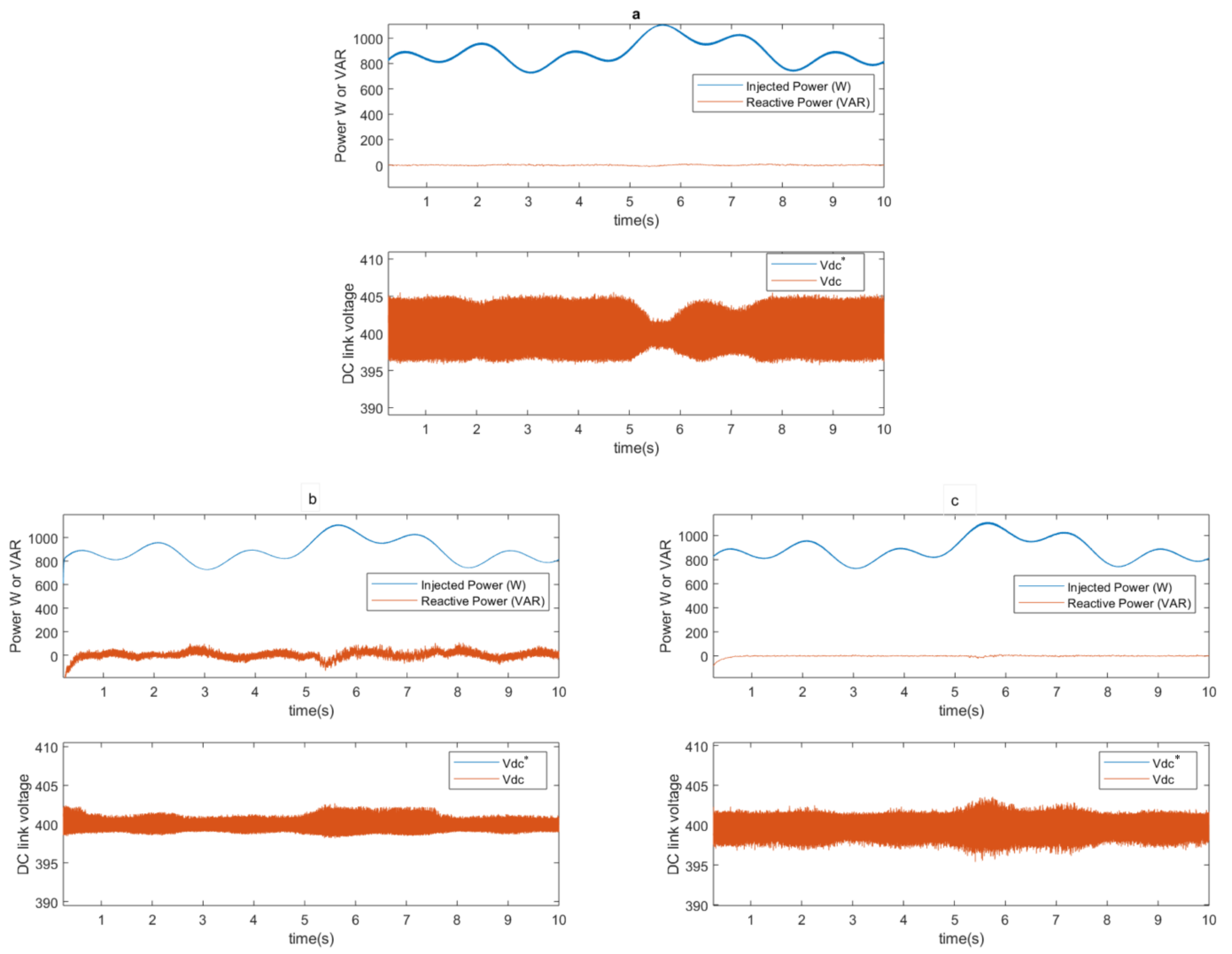
4.2. Results with Variable Power

In order to simulate the variability of collected wind power, we tested the algorithms with a sinusoidal wind model [44] where the time evolution of the wind speed $V_w$ was given by:

$$V_w=A_0+\sum _{i=1}^4{A}_{i}sin\left(\frac{2\pi t}{T_i}\right)$$

(32)

where the value of the coefficients $A_i$ and $T_i$ are reported in

Table 3. Values of the parameters for the wind model.

index	i	0	1	2	3	4
Amplitude	$A_i$	9.0	0.2	2.0	1	0.2
Period	$T_i$		0.11	0.28	1.29	10.00

.

The mechanical power $P_m$ supplied by the wind turbine to the electrical generator can be expressed as [44]:

$$P_m=\frac{1}{2}{C}_p\rho A{V}_w^3$$

(33)

where $C_p$ is the power coefficient of the turbine, A is the area of the turbine, and $\rho$ is the air density. In our study, we assumed that the WECS extracts the maximum mechanical power; in other words, that $C_p$ is maintained at its maximum value. The term $\frac{1}{2}{C}_p\rho A$ is, thus, a constant that has been adjusted in order to model the maximum mechanical power of $1$kW. In addition, we assumed that the electrical generator is ideal, which implies that $P_s=P_m$. Thus, the current $i_s$ that the DC source must provide to the grid-side converter in our simulation and experimental bench was calculated from the value $P_s$ deduced from the sinusoidal wind model and the DC-link voltage value.

Figure 7 shows the simulation results for the three algorithms with a value for the DC link capacity of $30\mathsf{\mu }$F. As in the first scenario, we observe in

Table 4. Comparison of the errors, ${ϵ}_{max}$ and ${ϵ}_{RMS}$, and the THD line current obtained by the three algorithms in the case of variable power.

Indicators	C	Variable Power
		Linear Control	SMC1	SMC2
${ϵ}_{max}$	$6\mathsf{\mu }$F	$41.1$	$6.7$	$7.1$
	$12\mathsf{\mu }$F	$19.2$	$3.8$	$3.8$
	$30\mathsf{\mu }$F	$5.6$	$2.3$	$3.3$
	$60\mathsf{\mu }$F	$2.9$	$1.8$	$2.4$
	$120\mathsf{\mu }$F	$1.9$	$1.7$	$1.2$
${ϵ}_{RMS}$	$6\mathsf{\mu }$F	$6.7$	$0.4$	$0.7$
	$12\mathsf{\mu }$F	$2.5$	$0.3$	$0.4$
	$30\mathsf{\mu }$F	$0.8$	$0.2$	$0.2$
	$60\mathsf{\mu }$F	$0.4$	$0.2$	$0.2$
	$120\mathsf{\mu }$F	$0.2$	$0.2$	$0.2$
THD (%)	$6\mathsf{\mu }$F	$1.7$	$2.3$	$1.1$
	$12\mathsf{\mu }$F	$1.2$	$2.3$	$1.1$
	$30\mathsf{\mu }$F	$1.2$	$1.8$	$1.3$
	$60\mathsf{\mu }$F	$1.1$	$2.6$	$1.1$
	$120\mathsf{\mu }$F	$1.1$	$2.7$	$1.2$

that SMC1 and SMC2 had good control on the $V_{dc}$ voltage since SMC1 and SMC2 generated an error ${ϵ}_{max}$ that changed between $1.2$ V and $7.1$ V when the value of the capacity decreased, and ${ϵ}_{RMS}$ remained relatively low and varied between $0.2$ V and $0.7$ V. The linear control generated exponentially increasing errors with the decrease of the capacity with an error ${ϵ}_{max}$ of $41.10$ V and ${ϵ}_{RMS}$ of $6.7$ V when $C=6\mathsf{\mu }$F.

For the case of THD, we notice that, as in the first scenario, the linear control and SMC2 had good performances in terms of the quality of the current injected into the power grid with a THD that did not exceed a maximum of $1.7\%$ when $C=6\mathsf{\mu }$F. However, this was not the case for SMC1, which suffered from a relatively higher THD, which was around $2.4\%$ due to its control nature (the chattering phenomenon).

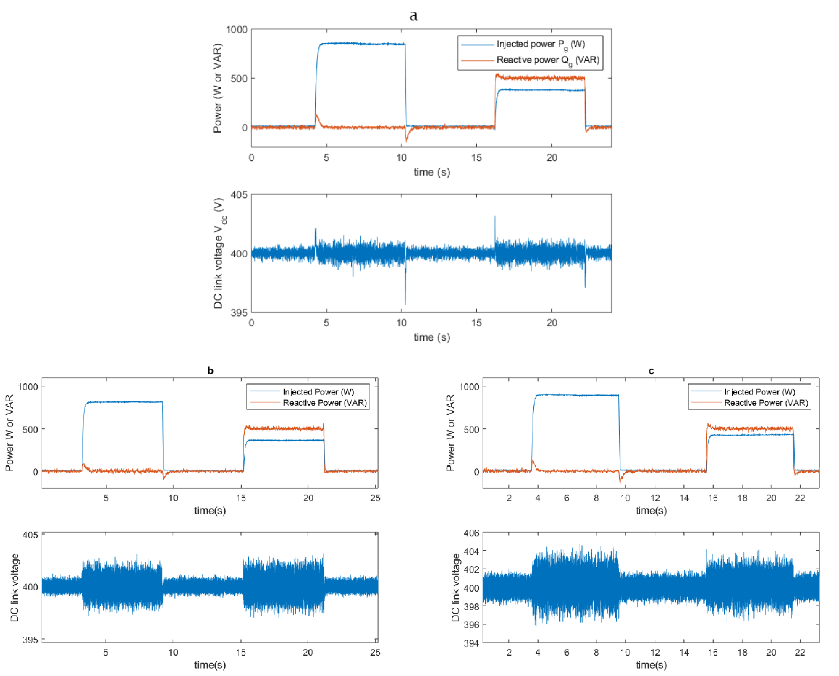
5. Experimental Results

5.1. Experimental Setup

The experimental bench was set up in accordance with the conversion chain described at the beginning of Section 4 (see Figure 8). The voltage and current probes measured the required signals at the location displayed in Figure 1. Experimental tests were conducted to validate the simulation results and the robustness of these algorithms under real operating conditions, including imperfections and measurement noise.

5.2. Results with a Step Power

As in the simulation setup, no power was injected at the beginning; then, suddenly, 900 W was injected for 6 seconds; and later, 400 W was injected and, at the same time, a reactive power of 500 VAR was required for 6 s. Figure 9 shows the experimental results for the three algorithms with a value for the DC-link capacity of $30\mathsf{\mu }$F.

Table 5. Comparison of the errors, ${ϵ}_{max}$ and ${ϵ}_{RMS}$, and the THD line current obtained by the three algorithms in the case of step power under a real experiment.

Quantity	C	Step Power
		$\mathit{P}>0$ and $\mathit{Q}=0$			$\mathit{P}>0$ and $\mathit{Q}>0$
		Linear Control	SMC1	SMC2	Linear Control	SMC1	SMC2
${ϵ}_{max}$	$6\mathsf{\mu }$F	$11.2$	$2.8$	$4.6$	$5.6$	$2.8$	$4.8$
	$12\mathsf{\mu }$F	$5.7$	$2.7$	$4.4$	$3.4$	$2.6$	$4.5$
	$30\mathsf{\mu }$F	$4.4$	$2.4$	$4.1$	$2.9$	$2.4$	$4.1$
	$60\mathsf{\mu }$F	$2.4$	$1.1$	$3.5$	$1.5$	$1.2$	$3.7$
	$120\mathsf{\mu }$F	$1.2$	$0.8$	$2.2$	$0.9$	$0.6$	$1.8$
${ϵ}_{RMS}$	$6\mathsf{\mu }$	$1.9$	$0.4$	$1.8$	$0.7$	$0.7$	1
	$12\mathsf{\mu }$	$1.2$	$0.4$	$1.4$	$0.6$	$0.5$	$0.8$
	$30\mathsf{\mu }$	$0.7$	$0.3$	$0.6$	$0.4$	$0.3$	$0.6$
	$60\mathsf{\mu }$	$0.4$	$0.2$	$0.6$	$0.2$	$0.2$	$0.3$
	$120\mathsf{\mu }$	$0.2$	$0.2$	$0.5$	$0.2$	$0.1$	$0.3$
THD (%)	$6\mathsf{\mu }$F	$7.5$	$8.7$	$9.1$	$11.7$	$11.5$	$12.5$
	$12\mathsf{\mu }$F	$7.9$	$9.2$	$9.1$	$12.2$	$12.1$	$12.6$
	$30\mathsf{\mu }$F	$8.2$	$9.5$	$8.2$	$12.5$	$12.5$	$11.9$
	$60\mathsf{\mu }$F	$8.1$	$8.5$	$8.3$	$12.2$	$11.8$	$12.2$
	$120\mathsf{\mu }$F	$8.7$	$8.5$	$8.5$	$12.6$	$12.1$	$12.6$

reports a comparison of the indicators, ${ϵ}_{max}$ and ${ϵ}_{RMS}$, and the THD line current obtained by the three algorithms in the case of step power: when only active power was injected ($P_g\approx 900$W and $Q_g=0$), and when the active power was injected and reactive power was requested ($P_g\approx 500$W and $Q_g\approx 400$W).

In the case when only active power was injected, we observed, for the linear control that ${ϵ}_{max}$ increased strongly as the capacity decreased to reach $11.2$V when $C=6\mathsf{\mu }$F. This behavior can theoretically be explained by the fact that ${\tau }_v$ sets the response time of the controller but not the overshoot. For the nonlinear control strategies, the overshoot was much less underlined as the capacity decreased; in the case of SMC1, there was almost no effect observed as the capacity decreased.

However, the conclusions are somewhat different when we analyze ${ϵ}_{RMS}$, which takes into account the fast fluctuation observed on $V_{dc}$. The evolution of ${ϵ}_{RMS}$ shows that the linear control and SMC2 behaved almost the same: in both cases, ${ϵ}_{RMS}$ increased slowly when the capacity decreased to reach around $1.9$V for the linear control and $1.8$V for SMC2 when $C=6\mathsf{\mu }$F. In the case of SMC1, ${ϵ}_{RMS}$ remained lower than 0.5 V as the capacity decreased.

The discrepancy between the simulation and experimental results resides in the quality of the power step: the power step in simulation was perfect, which consequently generated significant overshoots of the DC-link voltage; on the contrary, a rise in time appeared in the experimental power step, which considerably reduced the voltage overshoots.

In addition, we report that the THD values were relatively high regardless of the controller; however, the performance can be compared relatively between controllers. We observed that the linear controller proved to be the most efficient with a THD of around $8\%$ against $9\%$ for nonlinear controllers. To justify such a result, it is worth noting that the SVM (see Figure 2) exploits the real value of $V_{dc}$ to generate the proper voltage at the output of the two-level inverter.

Consequently, the slow variations of the voltage $V_{dc}$ observed mainly on the linear control can be compensated by the SVM. On the contrary, the quick fluctuations on the voltage $V_{dc}$ were not as well compensated by the SVM, which explains why the SMC1 and SMC2 controllers were less efficient. The THD on the grid voltage was around $3\%$ in the different experiments, while perfect sinusoidal sources were considered in the simulations.

In the case when active power was injected and reactive power was required ($P_g\approx 400$W and $Q_g\approx 500$VAR), we observed that the difference between the three controllers concerning the errors ${ϵ}_{max}$ and ${ϵ}_{RMS}$ on the DC-link voltage was reduced. In particular, the overshoot in the case of the linear controller was no more than $6$V, which was expected since the power injected was only $400$W.

The THD on the line currents was close between the different algorithms by around $12\%$—that is, 3 to $4\%$ more than in the case where only active power was injected. This result shows that the control of the reactive power, which was a priori carried out independently of the injected power had a significant impact on the quality of the line currents.

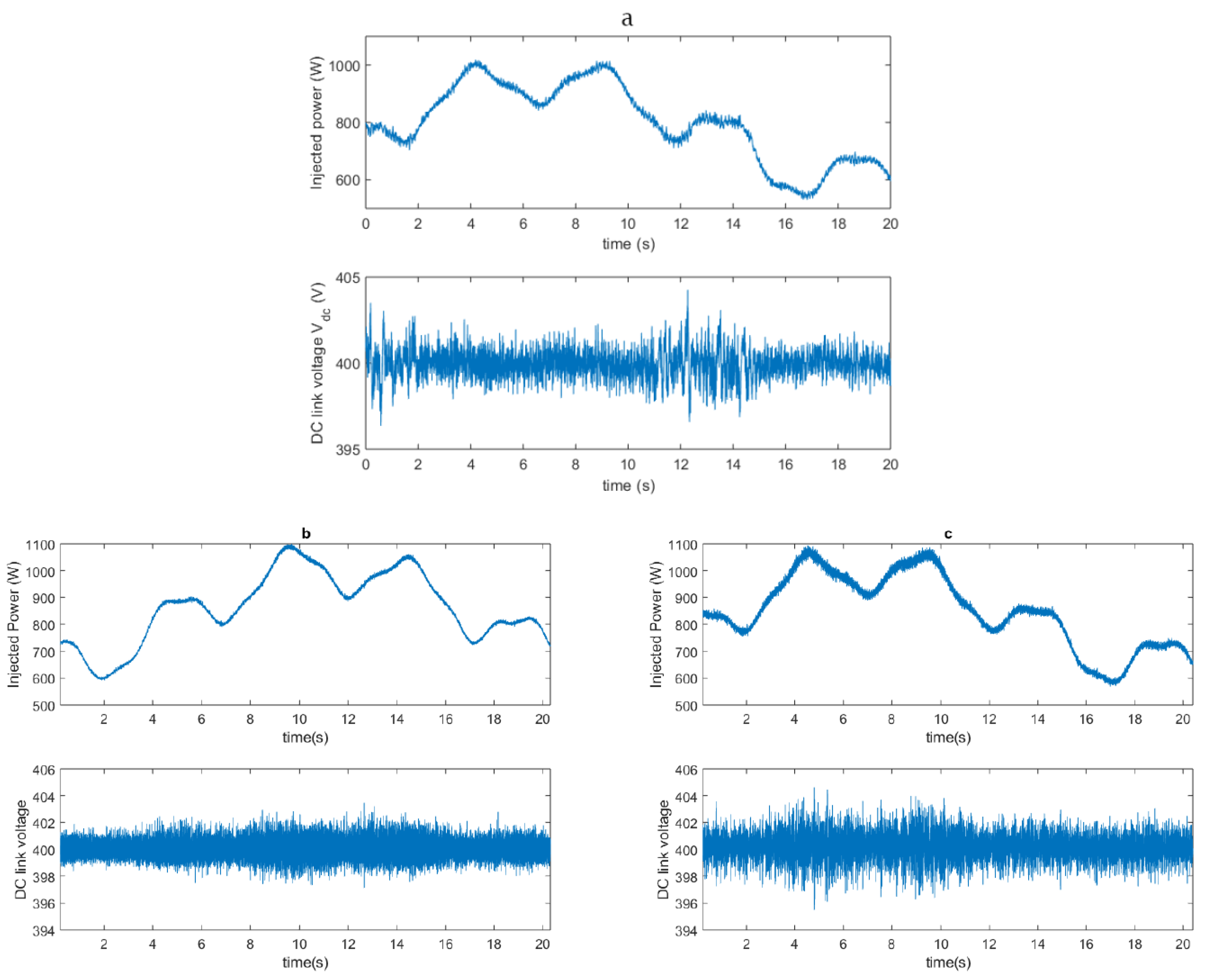
5.3. Results with Variable Power

As in the simulation, we tested the three algorithms with the sinusoidal wind model for different values of the DC-link capacity between $12\mathsf{\mu }$F and $120\mathsf{\mu }$F. Figure 10 shows the experimental results obtained by the three algorithms with a value for the DC-link capacity of $30\mathsf{\mu }$F.

The experimental value of the indicators ${ϵ}_{max}$ and ${ϵ}_{RMS}$ are reported in

Table 6. Comparison of the errors, ${ϵ}_{max}$ and ${ϵ}_{RMS}$, and the THD line current obtained by the three algorithms in a real experiment under a real regime.

Indicators	C	Variable Power
		Linear Control	SMC1	SMC2
${ϵ}_{max}$	$12\mathsf{\mu }$F	$6.9$	$2.9$	$4.5$
	$30\mathsf{\mu }$F	$4.8$	$2.7$	$4.1$
	$60\mathsf{\mu }$F	$4.1$	$1.8$	$3.9$
	$120\mathsf{\mu }$F	$3.7$	$1.3$	$3.5$
${ϵ}_{RMS}$	$12\mathsf{\mu }$F	$1.1$	$0.4$	$1.2$
	$30\mathsf{\mu }$F	$0.8$	$0.2$	$0.8$
	$60\mathsf{\mu }$F	$0.7$	$0.1$	$0.8$
	$120\mathsf{\mu }$F	$0.4$	$0.1$	$0.7$
THD (%)	$12\mathsf{\mu }$F	$7.9$	$8.9$	$10.1$
	$30\mathsf{\mu }$F	$8.1$	$9.1$	$9.2$
	$60\mathsf{\mu }$F	$8.2$	$9.4$	$9.5$
	$120\mathsf{\mu }$F	$9.5$	$10.1$	$9.4$
Efficiency $\eta$ (%)	$12\mathsf{\mu }$F	$94.1$	$93.9$	$94.1$
	$30\mathsf{\mu }$F	94	$92.8$	$94.1$
	$60\mathsf{\mu }$F	$93.78$	$93.40$	$93.81$
	$120\mathsf{\mu }$F	$92.9$	$91.8$	$92.9$

. We observed that, as in Section 4.2, the SMC1 algorithm ensured better control of the DC-link voltage: the value of ${ϵ}_{max}$ changed between $1$V and $3$V depending on the value of the capacity, while ${ϵ}_{max}$ changed between $3.7$V and $7$V for the linear control and changed between $3.5$ V and $4.5$ V for SMC2. The value of ${ϵ}_{RMS}$ measured over 20 s was also the smallest for SMC1.

Table 6 shows the performance of the different controllers on the grid-side in terms of distortion of the line currents and efficiency $\eta =P_g/P_s$ of the conversion chain from the capacity to the network. As observed in the case of a power step, the THD on the line currents was not necessarily lower when the voltage control indicators ${ϵ}_{max}$ and ${ϵ}_{RMS}$ were smaller; we observed, once again, that the linear controller had slightly better performance compared with the nonlinear controllers.

The efficiency of the grid-side converter with SMC1 was lower by around $1\%$ when compared to the linear controller and SMC2. This result can be explained by the fact that SMC1 generates a very variable command despite the introduction of the smooth function in Equation (19) to reduce the effect of chattering; the number of transistors switching in the inverter is then greater, which induces more losses.

6. Conclusions

In this article, we performed a comparative study of linear and nonlinear algorithms designed for the grid-side control of the power flow in a WECS. Both the simulation results and experimental tests were performed with the given power scenarios for different values of the DC-link capacity with the DC storage element being the key element of the grid-side converter. Only algorithms whose theory guaranteed accuracy and stability were studied.

The simulation and experimental results demonstrated that SMC1 was the most efficient algorithm for controlling the DC-link voltage with a maximum error that did not exceed $3\%$ when $C=6\mathsf{\mu }$F for both power injection scenarios, while the linear control suffered from an overshoot that increased exponentially with the decrease in capacity, reaching ${ϵ}_{max}=11.2\%$ when $C=6\mathsf{\mu }$F. However, SMC1 did not translate its efficiency into better side-grid performance: the THD was slightly degraded ($THD=8.9\%$ when $C=6\mathsf{\mu }$F) compared to linear control ($THD=7.9\%$ when $C=6\mathsf{\mu }$F), while the system efficiency was slightly lower, where $\eta$ was $93.9\%$ and $94.1\%$ for the SMC1 and linear control, respectively.

These disadvantages of SMC1 can be explained by the nature of the command that generates chattering. The linear control was designed from the internal model control theory where an active damping was added to avoid steady state error. The DC-link voltage control was less efficient than with SMC1; however, the smoother control led to better performance on the grid-side. Finally, SMC2 did not prove to be more efficient than SMC1, as ${ϵ}_{max}=4.5\%$ and $THD=10.1\%$ when $C=6\mathsf{\mu }$F.

However, an additional measurement of the current supplied by the generator-side converter is theoretically necessary to ensure the stability of SMC2. One possible explanation for the poorer results is that the modeling used here is too coarse for this type of command. Indeed, the model is based on the power conservation law where the inverter is supposed to be lossless. In the case of linear control and SMC1, these additional losses can be added in the perturbation term without incidence, while, for SMC2, the derivation of the command is theoretically no more valid.

References

1. Kabouris, J.; Kanellos, F.D. Impacts of Large-Scale Wind Penetration on Designing and Operation of Electric Power Systems. IEEE Trans. Sustain. Energy 2010, 1, 107–114. [Google Scholar] [CrossRef]
2. McKenna, R.; Leye, P.O.V.d.; Fichtner, W. Key challenges and prospects for large wind turbines. Renew. Sustain. Energy Rev. 2016, 53, 1212–1221. [Google Scholar] [CrossRef]
3. Menezes, E.J.N.; Araujo, A.M.; da Silva, N.S.B. A review on wind turbine control and its associated methods. J. Clean. Prod. 2018, 174, 945–953. [Google Scholar] [CrossRef]
4. Kumar, D.; Chatterjee, K. A review of conventional and advanced MPPT algorithms for wind energy systems. Renew. Sustain. Energy Rev. 2016, 55, 957–970. [Google Scholar] [CrossRef]
5. Tiwari, R.; Babu, N.R. Recent developments of control strategies for wind energy conversion system. Renew. Sustain. Energy Rev. 2016, 66, 268–285. [Google Scholar] [CrossRef]
6. Toledo, S.; Rivera, M.; Elizondo, J.L. Overview of wind energy conversion systems development, technologies and power electronics research trends. In Proceedings of the IEEE International Conference on Automatica, Curico, Chile, 19–21 October 2016. [Google Scholar]
7. Jain, B.; Jain, S.; Nema, R.K. Nema Control strategies of grid interfaced wind energy conversion system: An overview. Renew. Sustain. Energy Rev. 2015, 47, 983–996. [Google Scholar] [CrossRef]
8. Abouri, H.; Guezar, F.E.; Bouzahir, H. An Overview of Control Techniques for Wind Energy Conversion System. In Proceedings of the 7th International Renewable and Sustainable Energy Conference (IRSEC), Agadir, Morocco, 27–30 November 2019. [Google Scholar]
9. Baloch, M.H.; Wang, J.; Kaloi, G.S. A Review of the State of the Art Control Techniques for Wind Energy Conversion System. Int. J. Renew. Energy Res. 2016, 6, 1277–1295. [Google Scholar]
10. Errami, Y.; Ouassaid, M.; Maaroufi, M. A performance comparison of a nonlinear and a linear control for grid connected PMSG wind energy conversion system. Int. J. Electr. Power Energy Syst. 2015, 68, 180–194. [Google Scholar] [CrossRef]
11. Yaramasu, V.; Dekka, A.; Duran, M.J.; Kouro, S.; Wu, B. PMSG-based wind energy conversion systems: Survey on power converters and controls. IET Electr. Power Appl. 2017, 11, 956–968. [Google Scholar] [CrossRef]
12. Szczesniak, P.; Kaniewski, J. Power electronics converters without DC energy storage in the future electrical power network. Electr. Power Syst. Res. 2015, 129, 194–207. [Google Scholar] [CrossRef]
13. Chen, Z.; Guerrero, J.M.; Blaabjerg, F. A Review of the State of the Art of Power Electronics for Wind Turbines. IEEE Trans. Power Electron. 2009, 24, 1859–1874. [Google Scholar] [CrossRef]
14. Diaz, M.; Cardenas, R.; Espinoza, M.; Rojas, F.; Mora, A.; Clare, J.C.; Wheeler, P. Control of Wind Energy Conversion Systems Based on the Modular Multilevel Matrix Converter. IEEE Trans. Ind. Electron. 2017, 64, 8799–8810. [Google Scholar] [CrossRef]
15. Amin, M.M.; Mohammed, O.A. Development of High-Performance Grid-Connected Wind Energy Conversion System for Optimum Utilization of Variable Speed Wind Turbines. IEEE Trans. Sustain. Energy 2011, 2, 235–245. [Google Scholar] [CrossRef]
16. Beddar, A.; Bouzekri, H.; Babes, B.; Afghoul, H. Experimental enhancement of fuzzy fractional order PI+I controller of grid connected variable speed wind energy conversion system. Energy Convers. Manag. 2016, 123, 569–580. [Google Scholar] [CrossRef]
17. Soliman, M.A.; Hasanien, H.M.; Azazi, H.Z.; El-Kholy, E.E.; Mahmoud, S.A. An Adaptive Fuzzy Logic Control Strategy for Performance Enhancement of a Grid-Connected PMSG-Based Wind Turbine. IEEE Trans. Ind. Inform. 2019, 15, 3163–3173. [Google Scholar] [CrossRef]
18. Tremblay, E.; Chandra, A.; Member, S.; Lagace, P.J. Grid-Side Converter Control of DFIG Wind Turbines to Enhance Power Quality of Distribution Network. In Proceedings of the EEE Power Engineering Society General Meeting, Montreal, QC, Canada, 18–22 June 2006. [Google Scholar]
19. Wu, B.; Lang, Y.; Zarkari, N.; Kouro, S. Power Conversion and Control of Wind Energy Systems; IEEE Press: Hoboken, NJ, USA, 2011; Chapter 4; pp. 142–152. [Google Scholar]
20. Barambones, O.; Cortajarena, J.A.; Alkorta, P.; de Durana, J.M.G. A Real-Time Sliding Mode Control for a Wind Energy System Based on a Doubly Fed Induction Generator. Energies 2014, 7, 6412–6433. [Google Scholar] [CrossRef]
21. Merabet, A.; Ahmed, K.T.; Ibrahim, H.; Beguenane, R. Implementation of Sliding Mode Control System for Generator and Grid Sides Control of Wind Energy Conversion System. IEEE Trans. Sustain. Energy 2016, 7, 1327–1335. [Google Scholar] [CrossRef]
22. Zhang, J.; Cheng, M. DC link voltage control strategy of grid-connected wind power generation system. In Proceedings of the 2nd International Symposium on Power Electronics for Distributed Generation Systems, Hefei, China, 16–18 June 2010. [Google Scholar]
23. Benouareth, I.; Houabes, M.; Khelil, K. Fuzzy Logic Based P/Q Control Design for Grid- Connected Wind conversion System. In Proceedings of the International Conference on Wind Energy and Applications, Algiers, Algeria, 6–7 November 2018. [Google Scholar]
24. Douiri, M.R.; Essadki, A.; Cherkaoui, M. Neural Networks for Stable Control of Nonlinear DFIG in Wind Power Systems. Procedia Comput. Sci. 2018, 127, 454–463. [Google Scholar] [CrossRef]
25. Jday, M.; Haggège, J. Modeling and neural networks based control of power converters associated with a wind turbine. In Proceedings of the International Conference on Green Energy Conversion Systems (GECS), Hammamet, Tunisia, 23–25 March 2017. [Google Scholar]
26. Bounasla, N.; Hemsas, K.E. Second order sliding mode control of a permanent magnet synchronous motor. In Proceedings of the 14th International Conference on Sciences and Techniques of Automatic Control & Computer Engineering, Sousse, Tunisia, 20–22 December 2013; pp. 535–539. [Google Scholar] [CrossRef]
27. Corradini, M.L.; Fossi, V.; Giantomassi, A.; Ippoliti, G.; Longhi, S.; Orlando, G. Discrete time sliding mode control of robotic manipulators: Development and experimental validation. Control Eng. Pract. 2012, 20, 816–822. [Google Scholar] [CrossRef]
28. Alsmadi, Y.M.; Utkin, V.; Haj-ahmed, M.A.; Xu, L. Sliding mode control of power converters: DC/DC converters. Int. J. Control 2018, 91, 2472–2493. [Google Scholar] [CrossRef]
29. Gambhire, S.J.; Kishore, D.R.; Londhe, P.S.; Pawar, S.N. Review of sliding mode based control techniques for control system applications. Int. J. Dyn. Control 2021, 9, 363–378. [Google Scholar] [CrossRef]
30. Babaie, M.; Sharifzadeh, M.; Mehrasa, M.; Al-Haddad, K. Optimized based algorithm first order sliding mode control for grid-connected packed e-cell (PEC) inverter. In Proceedings of the 2019 IEEE Energy Conversion Congress and Exposition (ECCE), Baltimore, MD, USA, 29 September–3 October 2019; pp. 2269–2273. [Google Scholar] [CrossRef]
31. Utkin, V.; Poznyak, A.; Orlov, Y.; Polyakov, A. Conventional and high order sliding mode control. J. Frankl. Inst. 2020, 357, 10244–10261. [Google Scholar] [CrossRef]
32. Eker, I. Second-order sliding mode control with experimental application. ISA Trans. 2010, 49, 394–405. [Google Scholar] [CrossRef] [PubMed]
33. Beltran, B.; Benbouzid, M.E.H.; Ahmed-Ali, T. Second-order sliding mode control of a doubly fed induction generator driven wind turbine. IEEE Trans. Energy Convers. 2012, 27, 261–269. [Google Scholar] [CrossRef] [Green Version]
34. Zheng, E.H.; Xiong, J.J.; Luo, J.L. Second order sliding mode control for a quadrotor UAV. ISA Trans. 2014, 53, 1350–1356. [Google Scholar] [CrossRef] [PubMed]
35. Bartolini, G.; Ferrara, A.; Usai, E. Chattering avoidance by second-order sliding mode control. IEEE Trans. Automat. Contr. 1998, 43, 241–246. [Google Scholar] [CrossRef]
36. Benbouzid, M.; Beltran, B.; Mangel, H.; Mamoune, A. A high-order sliding mode observer for sensorless control of DFIG-based wind turbines. In Proceedings of the IECON—38th Annual Conference on IEEE Industrial Electronics Society, Montreal, QC, Canada, 25–28 October 2012. [Google Scholar]
37. Narayana, M.; Putrus, G.A.; Jovanovic, M.; Leung, P.S.; McDonald, S. Generic maximum power point tracking controller for small-scale wind turbines. Renew. Energy 2012, 44, 72–79. [Google Scholar] [CrossRef] [Green Version]
38. Ottersten, R. On Control of Back-to-Back Converters and Sensorless Induction Machine Drvies. Ph.D. Thesis, Chalmers University of Technology Goteborg, Goteborg, Sweden, 2003; pp. 90–93. [Google Scholar]
39. Yazdanian, M.; Mehrizi-Sani, A. Internal Model-Based Current Control of the RL Filter-Based Voltage-Sourced Converter. IEEE Trans. Energy Convers. 2014, 29, 873–881. [Google Scholar] [CrossRef]
40. Abubakar, U.; Mekhilef, S.; Mokhlis, H.; Seyedmahmoudian, M.; Horan, B.; Stojcevski, A.; Bassi, H.; Rawa, M.J.H. Transient faults in wind energy conversion systems: Analysis, modelling methodologies and remedies. Energies 2018, 11, 2249. [Google Scholar] [CrossRef] [Green Version]
41. Chung, S.-K. A Phase Tracking System for Three Phase Utility Interface Inverters. IEEE Trans. Power Electron. 2000, 15, 431–438. [Google Scholar] [CrossRef] [Green Version]
42. Perruquetti, W.; Barbot, J.-P. Sliding Mode Control in Engineering; CRC Press: Boca Raton, FL, USA, 2002. [Google Scholar]
43. Moreno, J.A.; Osorio, M. A lyapunov approach to a second-order sliding mode controllers and observers. In Proceedings of the 47th IEEE Conference on Decision and Control, Cancun, Mexico, 9–11 December 2008; pp. 2856–2861. [Google Scholar]
44. Aubree, R.; Auger, F.; Mace, M.; Loron, L. Design of an efficient small wind-energy conversion system with an adaptive sensorless MPPT strategy. Renew. Energy 2016, 86, 280–291. [Google Scholar] [CrossRef]
Figure 1. Structure of the grid-side conversion system.
Energies 14 04049 g001
Figure 2. Structure of the voltage oriented control (VOC) for the grid-side converter.
Energies 14 04049 g002
Figure 3. Regulation loop for linear control with active damping.
Energies 14 04049 g003
Figure 4. SMC1 controller block diagram.
Energies 14 04049 g004
Figure 5. SMC2 controller block diagram.
Energies 14 04049 g005
Figure 6. Response of the grid-side converter in the transient regime for C = 30 μ F. (a) PI controller, (b) SMC1 controller, and (c) SMC2 controller.
Energies 14 04049 g006
Figure 7. Response of the grid-side converter in the variable regime with C = 30 μ F. (a) PI controller; (b) SMC1 controller; and (c) SMC2 controller.
Energies 14 04049 g007
Figure 8. The experimental setup of the system.
Energies 14 04049 g008
Figure 9. Response of the grid-side converter in the transient regime with the (a) linear controller, (b) SMC1 controller; and (c) SMC2 controller for C = 30 μ F.
Energies 14 04049 g009
Figure 10. Responses of the grid-side converter in the variable regime with the (a) linear controller, (b) SMC1 controller; and (c) SMC2 controller for C = 30 μ F.
Energies 14 04049 g010