Modeling of Harmonic Current in Electrical Grids with Photovoltaic Power Integration Using a Nonlinear Autoregressive with External Input Neural Networks

Abstract

This research presents the modeling and prediction of the harmonic behavior of current in an electric power supply grid with the integration of photovoltaic power by inverters using artificial neural networks to determine if the use of the proposed neural network is capable of capturing the harmonic behavior of the photovoltaic energy integrated into the user’s electrical grids. The methodology used was based on the use of recurrent artificial neural networks of the nonlinear autoregressive with external input type. Work data were obtained from experimental sources through the use of a test bench, measurement, acquisition, and monitoring equipment. The input–output parameters for the neural network were the current values in the inverter and the supply grid, respectively. The results showed that the neural network can capture the dynamics of the analyzed system. The generated model presented flexibility in data handling, allowing to represent and predict the behavior of the harmonic phenomenon. The obtained algorithm can be transferred to physical or virtual systems for the control or reduction of harmonic distortion.

1. Introduction

Renewable energies are considered clean, abundant, and increasingly competitive energies. They differ from fossil fuels mainly in their diversity, profusion, and harnessing the potential in all regions of the planet, but above all, in that they do not generate greenhouse gases and polluting emissions [1].

Photovoltaic solar (PV) is one of the renewable energy sources, which involves the direct transformation of solar radiation into electrical energy; this transformation is achieved by leveraging the properties of semiconductor materials such as silicon, which can generate electrical power when ionized by solar radiation [2].

PV generation systems are classified into two large groups: isolated and interconnected [3]. In the former, the generation is not connected in any way to the electric supply grid, while in the latter, the energy generated is integrated into the grid by the use of electronic power inverters.

Inverters used in interconnected PV systems have the main function of converting direct waveform power (DC) parameters into sinusoidal alternating waveform (AC) parameters [4]. These devices generate various power quality problems, due to the nonlinear behavior of their components and their operational characteristics [5,6], among which are transients and voltage variations, flickering, harmonic, and interharmonics.

Among some of the harmful effects produced by harmonic distortion in currents and/or voltages are the increase in Joule effect losses in electric feeders, overheating in grounded conductors, in motors, generators, transformers and cables, reducing their service life, vibration in electrical machines, failure of capacitor and transformer banks, resonance effects, as well as operational problems in sensitive electronic devices and interference in telecommunications systems [7].

Due to the imminent growth in the use of PV systems interconnected to power grids, which have led to an increase in energy quality problems [8], specifically those caused by harmonic distortion, it is necessary to characterize and model harmonic behavior due to the integration of the PV power in order to control and/or suppress the content of harmonic distortion at the common coupling point (CCP), as well as in the power supply grid.

1.1. Related Works

Various research studies have been developed on the modeling of harmonic behavior in electrical networks with power integration coming from PV generation systems, both in medium and low voltage. An alternative model of an interactive PV system that can be used to characterize the harmonics of such systems when connected to distorted and undistorted grids, respectively, was presented in [9]. The proposed model was based on the concept of harmonic domain. The real expansion of the Fourier series and the complex Fourier series were used for this model. Flexible harmonic domain models of a three-phase PV system for stable state analysis have been developed [10], based on a selection of dominant harmonics and the reordering of the Toeplitz type matrix involved in frequency convolution. On the other hand, in [11], the authors presented harmonic modeling using a mathematical analysis of a harmonic study of different parallel PV systems connected to a low voltage distribution network to identify the potential resonance between PV inverters and system impedance, while in [12], a novel model was shown in the time domain, using average functions and a novel switching emulator. Despite the results obtained, these models are not suitable when trying to represent the behavior of nonstationary signals due to the limitations presented by mathematical tools such as the transformed and Fourier series.

On the other hand, ANNs have traditionally been used for the detection, classification, and control of energy quality problems, especially those related to harmonic voltage and current distortion, as well as in systems that aim to control and/or eliminate such phenomena. A radial basis function ANN for harmonic load identification was implemented with several of the training and testing data from the combination of 15 different load types to validate the accuracy and efficiency of the proposed algorithm [13]. For the detection and classification of energy quality disturbances [14], the processing of voltage or current signals was used using a phase estimation model, while the classification task was performed using threshold-based rules and an ANN; similar studies [15] that also aim to detect and classify energy quality problems have used the Hilbert–Huang transform and a Perceptron multilayer ANN. With regard to the use of ANN for harmonic control and disposal, the authors of [16] proposed a new ANN structure based on regression by least squares of gradient descent for the control of a PV solar system, integrated into the grid with improved power quality. Another study used a delta–bar–delta ANN-based control [17] to optimally operate by feeding active energy to loads and the remaining power to the grid based on static distribution compensator capabilities, such as harmonic mitigation, load balancing, and power factor improvement. While ANNs have proven their efficiency when used for identification and classification processes, the ANN topologies used have not been suitable for modeling and predicting time-variant systems.

When it comes to modeling and predicting the behavior of load current harmonics injected into power energy micro-networks, self-regressive nonlinear artificial neural networks with exogenous input (NARX neural network) [18] have been used, which performed well in harmonic prediction. Similarly, the authors of [19] described the results of modeling and predicting total harmonic distortion of current and voltage for a nonlinear high power load; modeling was performed using intelligent neural-network-based techniques and diffuse inference, obtaining adequate results with very few errors. Based on the performance of this type of ANN, it is estimated that the application for the analysis of the harmonic behavior of the current in electrical networks with power integration from PV generation systems can deliver results of interest applicable in the field of study of the quality of electrical energy.

1.2. Scope and Contribution

This work shows the modeling and prediction of current behavior in a power grid under critical operating conditions when the CCP integrates powers from this grid with a PV system through a solid-state inverter, jointly powering resistive loads. The methodology used is based on the use of the NARX network, and the results may serve as a future guide for the control and/or suppression of harmonic content in the CCP of such systems.

ANN are computer algorithms that simulate the biological activity of neurons and the processing of human brain information [20]. They are distinguished in fields of science in which the conception of solutions or characteristics of problems analyzed are difficult to determine with conventional programming, such as image and voice processing, pattern recognition, planning, adaptive interfaces for human–machine systems, control and optimization, signal filtering, modeling and prediction [21]. According to their topology, they are classified into monolayers, multilayers, convolutional, radial based, and recurrent.

The recurrent neural networks (RNNs) do not have a layer structure (such as single-layer, multilayer, and convolutional networks) but allow arbitrary connections between neurons, even being able to create loops, thus establishing temporality and allowing the network to have memory [22]. The data that enter at a time “t” to the entry of the network are converted and transferred in it even in the later moments of time, i.e., $t+1$, $t+2$, $t+3\dots$ The architecture of this type of neural network has become a model implemented in different domains due to its natural ability to process sequential inputs and know their dependencies in the long term [23]. Unlike the conventional ANNs (forward), RNNs are connected to each other in the same hidden layer and a training function is applied repeatedly to hidden states [24]. RNNs are archetypes of deep learning (DL), which are repeatedly fed back.

In this regard, NARX networks have performed adequately in diverse applications, especially in sequential problems, as well as in dynamic system modeling and time series prediction [25,26,27]. Consequently, this type of architecture gives the training various advantages, such as greater network input accuracy and forward orientation; thus, static reverse propagation can be used [28].

The main contribution of this research lies in determining if an RNN (specifically that of the NARX type) presents an adequate functioning in the modeling and prediction of the behavior of the current in low voltage grids when it is integrated into electrical power from photovoltaic generation systems using electronic inverters; moreover, it contributes to establishing new methodologies based on artificial neural networks (ANNs) for the analysis of the harmonic current phenomenon whose presence is increasingly continuous in the face of the imminent increase in the use of nonconventional renewable energy sources such as solar and wind. In addition, the results obtained may be used in various investigations related to the power quality, as well as in the control and reduction of problems that affect electrical systems, specifically electrical distribution grids.

2. Methodology and Development

2.1. Overview of NARX

When the signals came from time series, some other topologies of ANNs have been successful; here, we can mention the NARXs networks [29]. A regular feedforward neural network contains time series of inputs in the input layer and predicts an output from the output layer [30]. Since RNNs are very complex [31], normally, the training and learning process may take a long period.

Our case is more adapted to the NARX, which is a commonly used discrete nonlinear system and can be mathematically represented as follows:

$$y\left(k\right)=f\left\{u\left(k-1\right),u\left(k-2\right),\dots ,u\left(k-l\right),y\left(k-1\right),y\left(k-2\right),\dots ,y\left(k-m\right)\right\}$$

(1)

where u(k) ϵ ℝ and y(k) ϵ ℝ denote the inputs and the outputs of the NARX model at the discrete time step, k, respectively. l ≥ 0 and m ≥ 0 are the input memory and the output memory used in the NARX model. The unknown function f(.), which is generally nonlinear, can be approximated, for instance, by a regular multilayer feedforward network. The resulting model architecture is called a NARX network or Jordan NARX network.

The network structure of the series–parallel mode Jordan NARX network (Jordan-SP) is presented in Figure 1. v1; v2; …; vn are the neurons in the hidden layer, W(i) is the weight matrix from the input layer to the hidden layer, and W(o) is the weight vector from the hidden layer to the output layer. The structure is a regular feedforward neural network (FNN) structure, in which the output’s regressor is formed only by the actual data of the system’s output.

$$\widehat{y}\left(k\right)=f\left\{u\left(k-1\right),u\left(k-2\right),\dots ,u\left(k-l\right),d\left(k-1\right),d\left(k-2\right),\dots ,d\left(k-m\right)\right\}$$

(2)

where d(k) is the desired or actual output data, and $\widehat{y}\left(k\right)$ is the network’s estimated output at the time step, k. The state of the p-th neuron and its output (x_p(k) are defined as

$$\begin{array}{c}{x}_p\left(k\right)={{\displaystyle \sum }}_{q=1}^{l+m+1}{w}_{pq}^{\left(i\right)}{u}_q\left(k\right)\\ v\left(k\right)=f\left(x_p\left(k\right)\right)\end{array}$$

(3)

where the subscripts stand for the index of the element in a vector or a matrix, $w_{pq}^{\left(i\right)}$ is the weight connecting the q-th input and the p-th neuron in the hidden layer. Then, the output of the network is

$$y\left(k\right)={\displaystyle \sum }_{p=1}^n{w}_p^{\left(o\right)}{v}_p\left(k\right)$$

(4)

The hyperbolic tangent sigmoid function is applied to the hidden layer and the linear function is applied to the output layer.

$$f\left(x\right)=\frac{2}{1+e^{-2x}}-1$$

(5)

In order to let the neural network model track the desired outputs, the cost function mean squared error (MSE) method is utilized here, which should be minimized between the desired outputs and the network’s estimated output. Thus, the cost function (J) for N steps is

$$J=\frac{1}{N}{\displaystyle \sum }_{k=1}^N{\left(\widehat{y}\left(k\right)-d\left(k\right)\right)}^2$$

(6)

which is a function of W(i) and W(o).

In the training process, for example, by using the Levenberg–Marquardt backpropagation algorithm [32], error functions in each time step can be calculated in parallel in one epoch as a regular FNN. Normally, an accurate training result is quickly achieved based on this network. However, since this type of network is generally only a one-step-forward predictor, it cannot be utilized in pure numerical simulations or as a reference model, which involves a long-term time prediction. Manual feedback of the output signal to the regressor without additional training may accumulate errors in every single step and finally cause instability.

In the equation for the NARX model, the next value of the dependent output signal y(k) is regressed on previous values of the output signal and previous values of an independent (MSE) input signal. A diagram of the resulting network is shown below (Figure 2), where a two-layer feedforward network is used for the approximation. This implementation also allows for a vector autoregressive with exogenous terms (ARX) model, where the input and output can be multidimensional.

You can consider the output of the NARX network to be an estimate of the output of some nonlinear dynamic system that you are trying to model. The output is fed back to the input of the feedforward neural network as part of the standard NARX architecture. As the true output is available during the training of the network, you could create a series–parallel architecture [33], in which the true output is used instead of feeding back the estimated output.

In this configuration, the errors are very small. However, because of the series–parallel configuration, these are errors for only a one-step-ahead prediction. A more stringent test would be to rearrange the network into the original parallel form (closed loop) and then to perform an iterated prediction over many time steps [33].

Now, the NARX (and other) networks must be converted from the series–parallel configuration (open loop), which is useful for training, to the parallel configuration (closed loop), which is useful for multi-step-ahead prediction.

All of the training is performed in open loop (also called series–parallel architecture), including the validation and testing steps. The typical workflow is to fully create the network in open loop, and only when it has been trained (which includes validation and testing steps) is it transformed to closed loop for multistep-ahead prediction.

You can now use the closed-loop (parallel) configuration to perform an iterated prediction in N time steps. In this network, you need to load the two initial inputs and the two initial outputs as initial conditions.

It is important to remark that each time a neural network is trained, it can result in a different solution due to different initial weight and bias values and different divisions of data into training, validation, and test sets. To ensure that a neural network of good accuracy has been found, retrain several times [33,34,35].

2.2. Experimental Setup

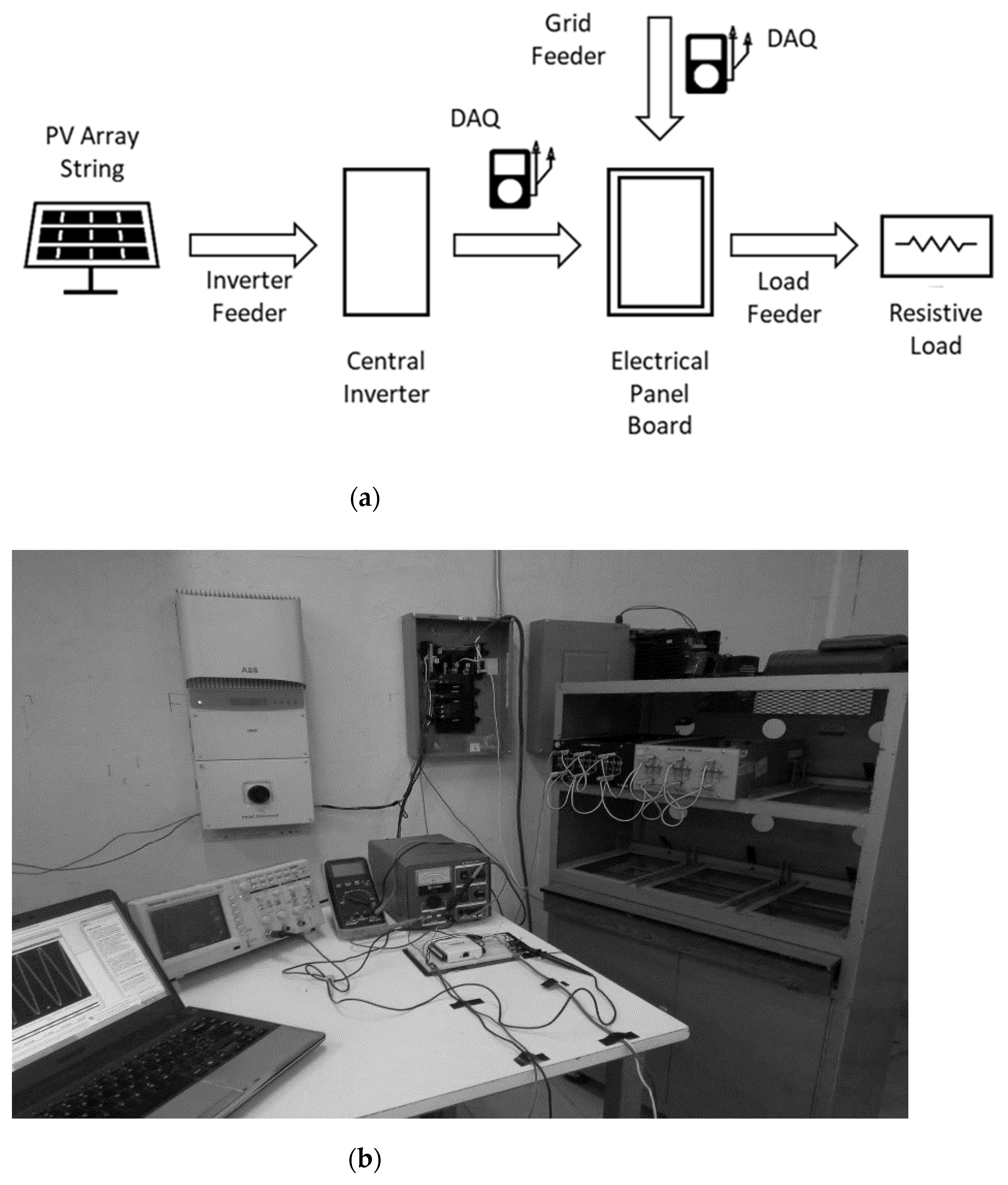
For the modeling and behavior prediction of current in the 220 V, 60 Hz power supply grid, at the CCP, where the powers of the grid and a PV system are integrated through electronic inverters, a test bench consisting of 6 monocrystalline solar panels of 250 W each was used in an arrangement of 1500 W. A central inverter interconnected to the grid, of the voltage-controlled type, with a full-bridge configuration of 3000 W capacity, 220 V_AC, 2 phases, and 3 wires was used. The CCP was located on a single-phase, 220 V, 100 A electric board, through which 530 W at 127 V resistive loads were fed (the configuration of the test bench—inverter type, load type, and generating power—was determined by applying an experimental design based on variance analysis and complete factorial designs). The harmonic current extraction stage was carried out by using Hall effect current sensors, model ACS712-20, and a USB-6008 NI data acquisition card, processing the information in SignalExpress software and finally generating the data to power the neural networks in a MATLAB environment.

Table 1. Current sensor characteristics.

	ACS712 Current Sensors
Imax	Sensitivity	Vout	Resolution
±5 A	185 mV/A	1575 V to 3425 V	26 mA
±20 A	100 mV/A	0.5 V to 4.5 V	49 mA
±30 A	66 mV/A	0.52 V to 4.48 V	74 mA

shows the ACS712 current sensor characteristics.

The experimental methodology for data acquisition and modeling of dynamic system behavior using ANN is as follows:

• Design and construction of the test bench;
• Connection and configuration of acquisition equipment;
• Data acquisition for references;
• Data acquisition for modeling;
• Determination of the ANN to be used;
• Structure of the ANN to be used;
• Application of ANN (training, validation, and testing of ANN);
• Obtaining results and conclusions.

Figure 3 shows the arrangement of the test bench elements.

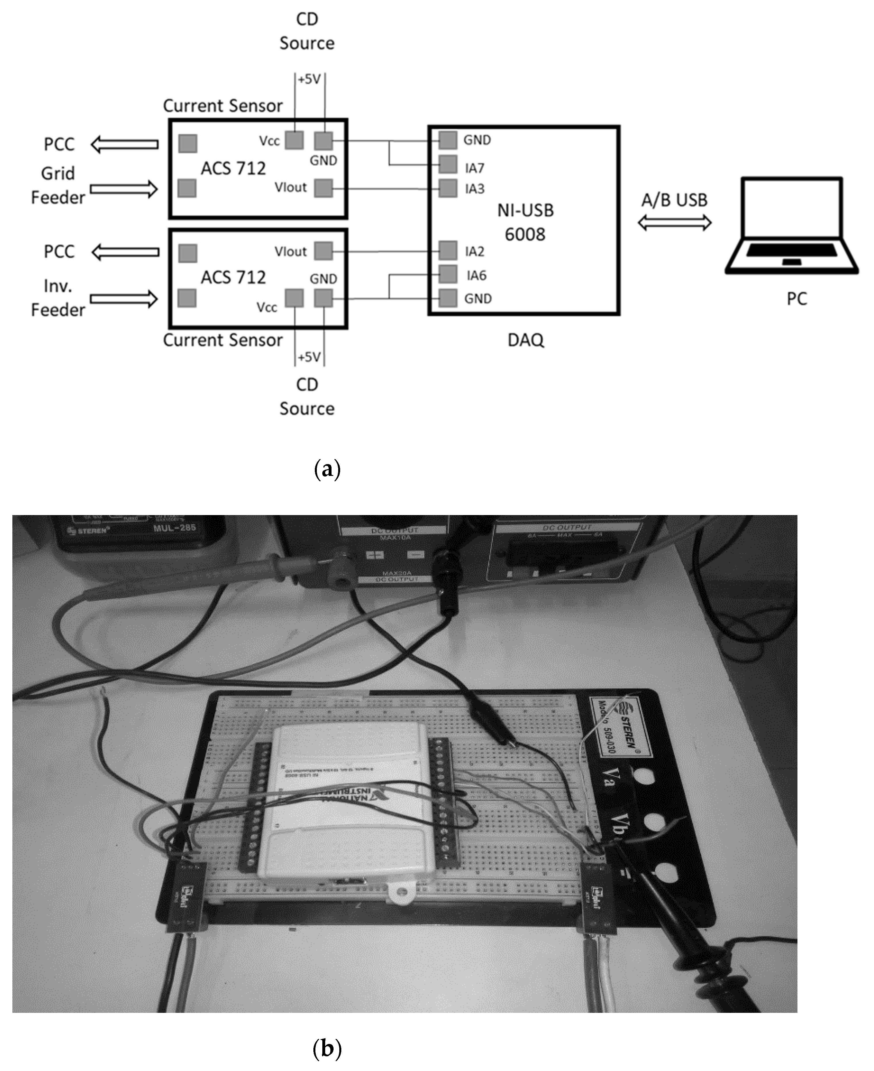
The phase conductors in each feeder (inverter and supply grid) were connected in series to the ACS712 current sensors, between their terminals: source (IP+) and load (IP−), with a polarization voltage of 5 V_DC between the Vcc and ground (GND) terminals of each sensor. Figure 4 shows the connection of data acquisition devices.

2.3. Data Acquisition

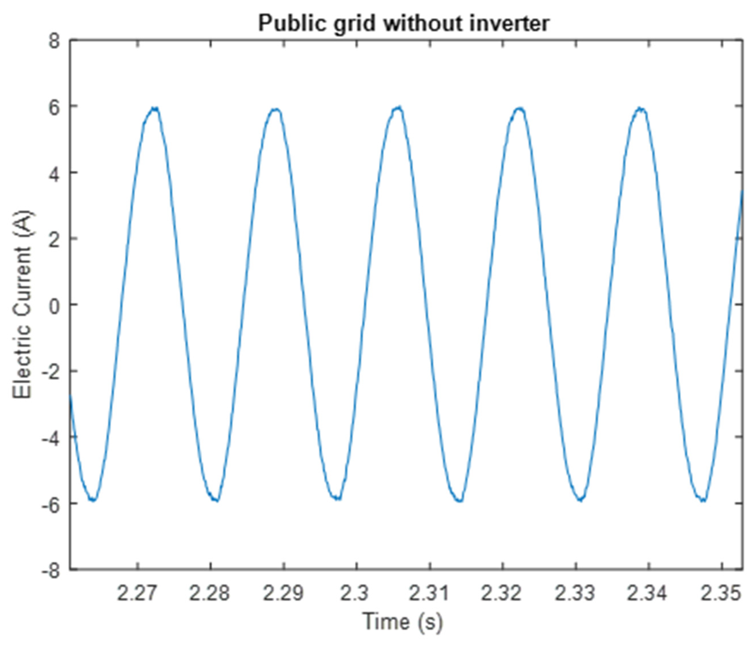
First, the data acquisition of the current parameters was performed in the grid feeder without power inputs from the PV system for 5 s, with a sample rate of 10,000 samples/second, to obtain reference information on the background harmonic distortion in the feeder, under the referred operating conditions. Second, data acquisition was carried out simultaneously of the current parameters in both feeders (supply grid and inverter), at CCP, with a sample rate of 5000 samples/second for each feeder for 5 s.

Table 2. Description and conditions for data acquisition.

Data Acquisition
No.	Description	Conditions of Acquisition
1	Supply grid feeder	No current input from the inverter and charging at CCP
2	Supply grid feeder	With input of current by the inverter and charging at CCP
3	Inverter feeder	With charging at CCP

shows the measurement points and signal acquisition conditions.

The figure above (Figure 5) shows a sinusoidal signal with a positive peak magnitude of 5.98 A, with little background harmonic distortion (THDi= 1.07%) and nondynamic (invariant in time) behavior.

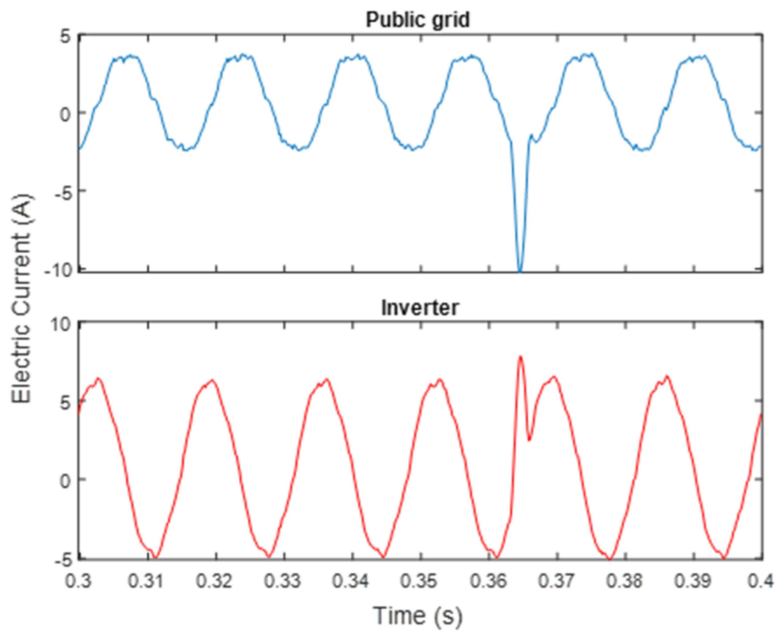
Figure 6 corresponds to the current in both feeders (supply grid and inverter), jointly feeding the resistive load. This graph shows the change in the waveform of the current signal in the supply grid in the face of the power integration of the PV system, using the electronic inverter. Both signals show distortion due to the presence of harmonics and nonlinear dynamic behavior.

2.4. NARX’s Structure

Since one of the characteristics of ANN is not having a single structure, this work used NARX networks configured with a series–parallel architecture (open loop) for the modeling network and in parallel (closed loop) for the prediction network, which was used to check the proper functioning of the resulting model [28]. Both networks are powered by input signals at the start of the network, containing two hidden layers with 10 neurons each, activated by sigmoid functions, and an output layer with a single neuron activated by a linear function. 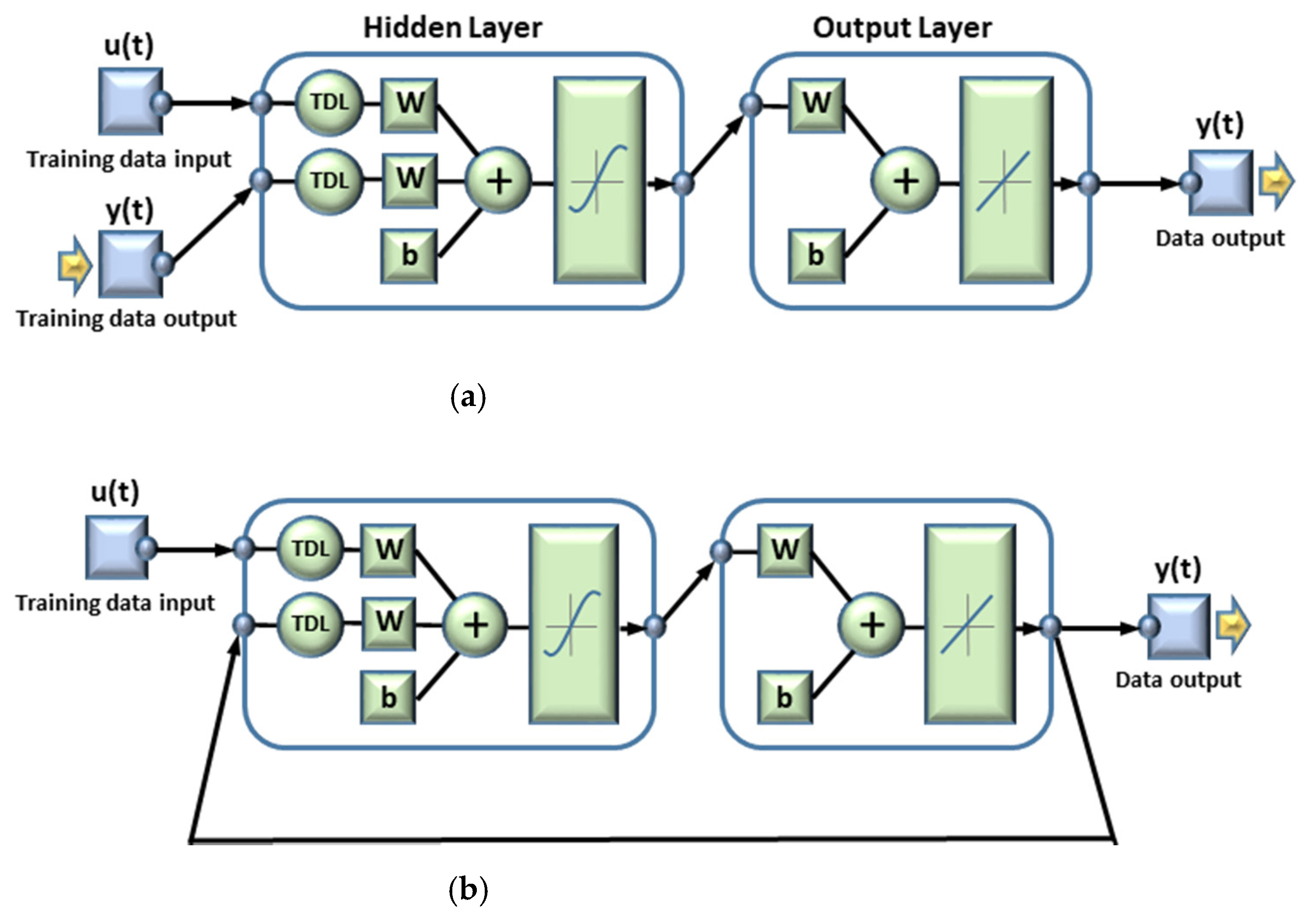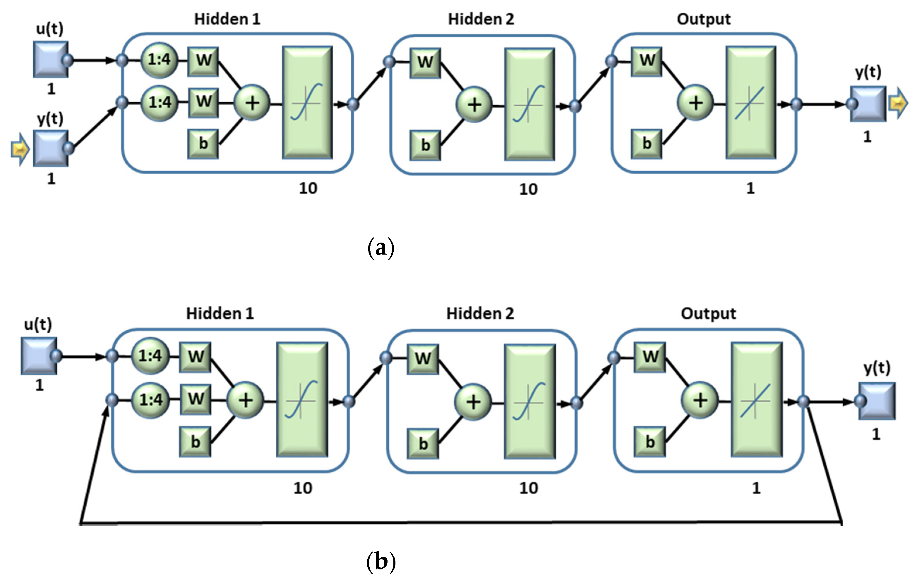Figure 7 shows the structures of the NARXs networks used. These networks have four variable offsets (shown by the 1:4 ratios in the tapped delay line (TDL)), which indicates that the input signals are made up of x(t), x(t − 1), x(t − 2), x(t − 3), and x(t − 4), and have input variables y(t − 1), y(t − 2), y(t − 3), and y(t − 4) for the series–parallel network, and z(t − 1), z(t − 2), z(t − 3), and z(t − 4) for the network in parallel, with “y” being the actual output and “z” the estimated output. The structure of the NARX network (the number of hidden layers, the number of neurons per layer, and the number of offsets) was determined by iteration of values to obtain the best performance of the network.

NARX network training is supervised, giving the network input patterns, as well as expected output (correct result). The input and output data consist of vectors line of 1 × 25,000 elements each and correspond to the magnitudes of currents in the inverter feeder (input data) and the magnitudes of currents in the electrical supply grid (expected output). The Levenberg–Marquardt algorithm was used as a training method, along with the MSE performance function, with a total of a thousand iterations (epochs, i.e., the number of times that the algorithms will be executed). The method used for calculating gradients was dynamic backpropagation.

The criteria for stopping training were mainly defined by the number of epochs (1000 iterations), gradient (less than 10⁻⁵), and 6 as the number of validation checks.

The general procedure in both networks consisted of the introduction of inputs (where the input neurons are activated); next, the information was propagated through the networks and outputs were generated, and then the outputs of the networks were compared to the desired outputs and the errors were calculated; finally, corrections were made to the weights that were based on these errors until they were minimized. During training, the dataset was randomly divided (to avoid an overfit effect), into three subsets for each network. The first subset was the training set, with this dataset network learning was carried out through weight adjustment and corresponded to 70% of the total data. The second subset (with 15% of the data) was the validation set that served to monitor the error during the training process. The last subset with the remaining 15% of the data was the test set, it was not used during training but was subsequently used to evaluate network performance [28].

3. Results and Discussion

After the parameterization of the series–parallel neural network, training was conducted using the Levenberg–Marquardt method using 269 iterations of the 1000 available epochs to obtain the lowest performance value before stopping the algorithm because six or more times, there were no changes in that performance during testing with validation data. Figure 8 exhibits a very fast drop in MSE, before 10 iterations.

The figure above shows how errors in training, validation, and test data follow the same trends during the algorithm run, finally achieving an MSE less than 10⁻²; in addition, it shows the minimum value of the network performance obtained in iteration 269, as 0.0067622; the similar behavior of the trends of the three data groups, the rapid decrease of the MSE, coupled with the fast ending of the algorithm, determine an adequate configuration and effectiveness of the NARX network.

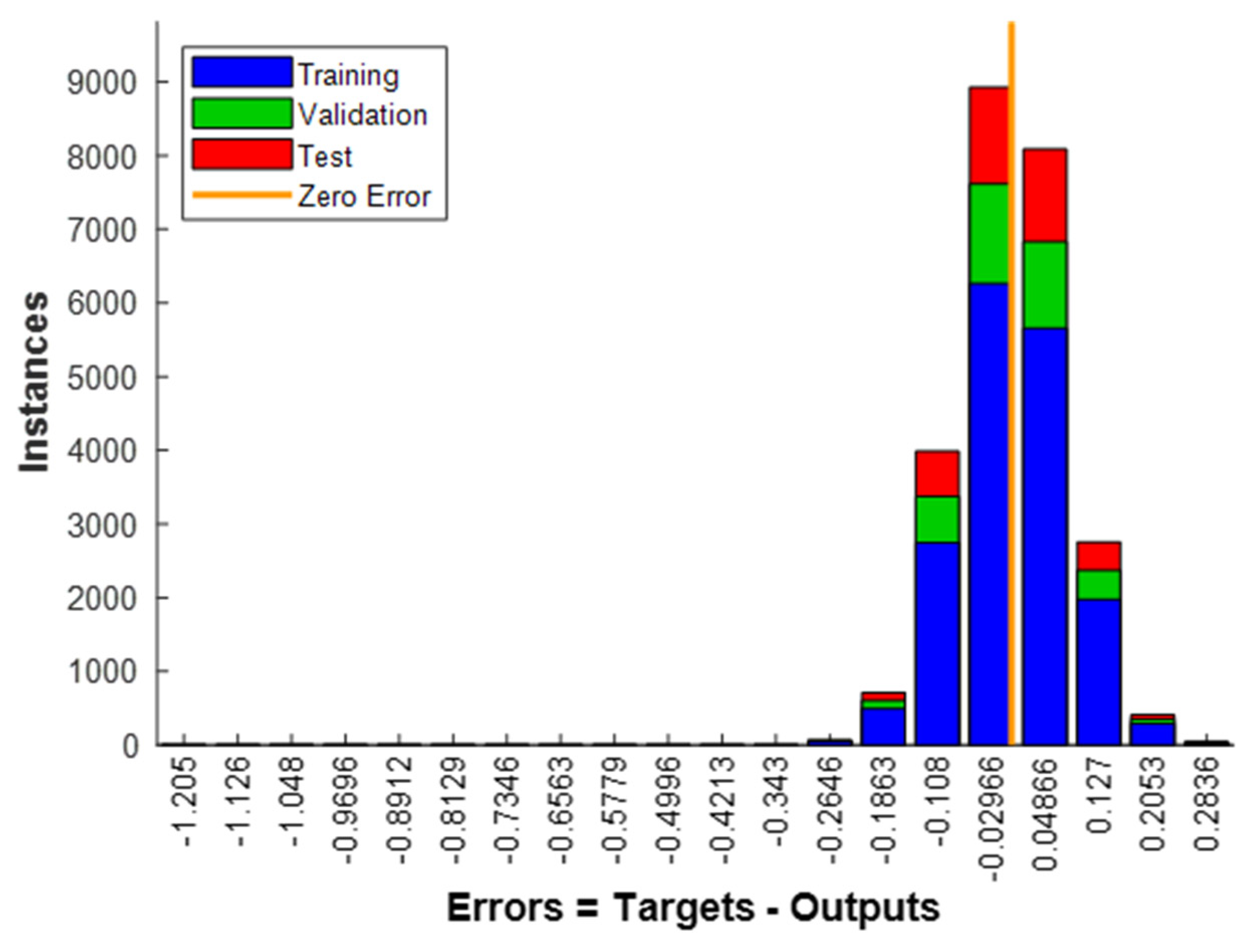
Figure 9 shows the histogram containing the errors in the three datasets; it is determined that on the centerline when the error is zero, the data ratio of the training set is higher, and this behavior is constant during the analysis of the data furthest from the null error, while always retaining the higher proportion of the training data in reference to validation and test data. This trend is also observed in the behavior of the data shown in Figure 8.

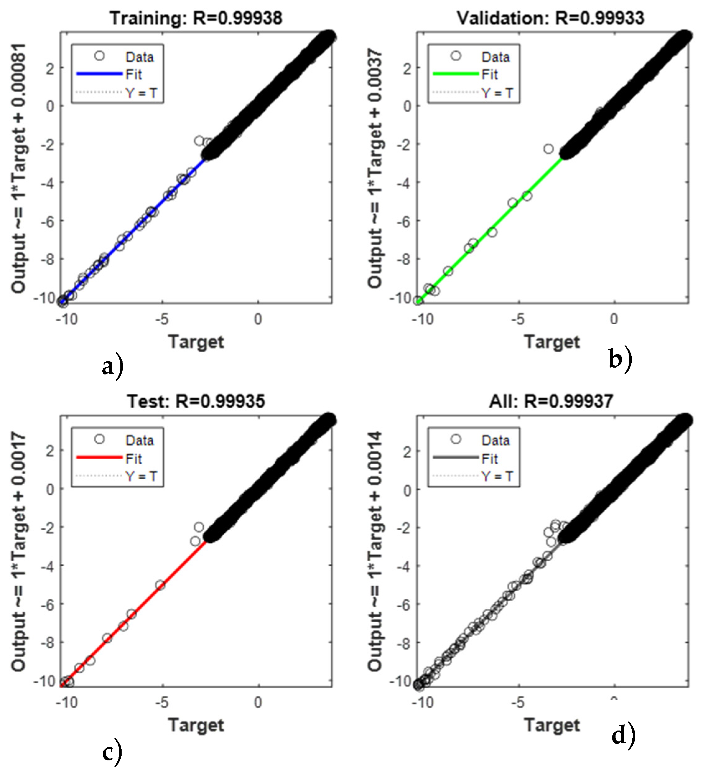
Another way to analyze the results of significant errors is using the linear regression method for each dataset (training, validation, and testing). Figure 10 shows the values between the achieved output and the required targets, which are far from the ideal linear adjustment (where the x-axis represents the target—in this case, the distorted signal measured in the network feeder—while on the y-axis represents the output value generated by the neural network); the best conditions are those of training data that have a 99.938% effectiveness in regression. This result can be attributed to a greater amount of data (70% of the total), with which the training was carried out. There is also a lot of proximity to the other data groups regarding the effectiveness of regression.

Subsequently, the temporary response obtained was evaluated by graphically relating the result of the NARX network, against the required values. Figure 11 shows the comparison between the results generated by each of the datasets against the target, in addition to the error present in each of moments of time. The response exhibits the characteristics of the difference between the current signal in the grid feeder in presence of power supplied by the PV system, and the response obtained by the NARX when the current signal enters it from the electronic inverter to the CCP. From the errors’ graph, it is observed that the differences between the target values and those resulting from the three training datasets are very close to zero, showing the biggest errors when signal behavior exhibits rapid and abrupt changes in its waveform.

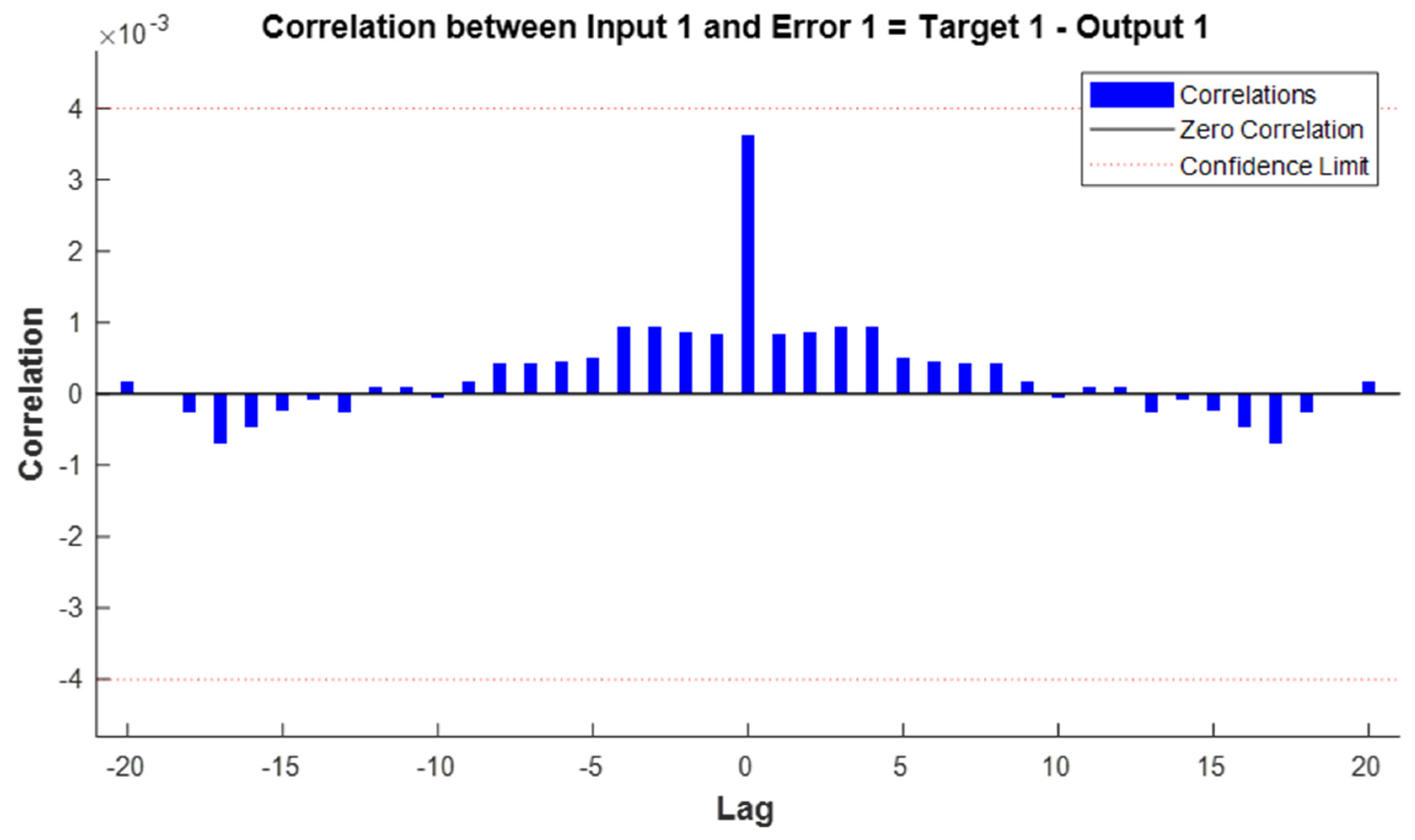
Finally, the correlation plots of errors with respect to time and inputs are displayed. Figure 12 presents error–time autocorrelation; it can be seen how the training is correct because the central correlation (MSE) with zero value is greater, while the rest are within the expected confidence limits.

Figure 13 shows the existence of a large number of correlations between inputs and error, which are within the limits, mostly concentrated in the zero value; thus, the training has optimal performance.

The configuration of the open-loop neural network is replaced with a closed-loop neural network (Figure 7b) in such a way that from the target inputs, the network uses its own predictions to check whether the model obtained through the open-loop network, has adequately defined the behavior of the current signal in the feeder of the electrical supply grid. This architecture produces results that differ from the temporal response of Figure 11 and depend on how appropriate the training has been. Now, the target values will be unknown, and the temporary response obtained will be the one shown in Figure 14.

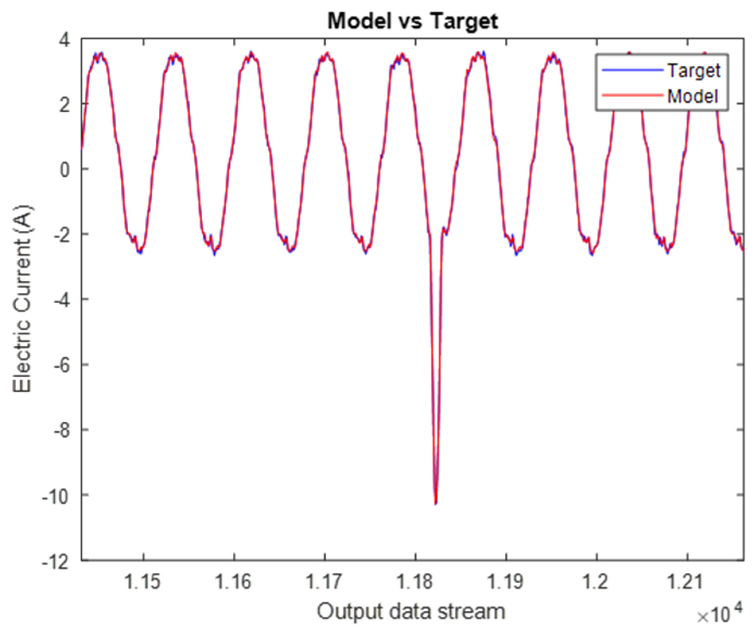
Figure 15 shows the comparison of the output of the open-loop network (model) against the target output. Similarity to Figure 14 can be seen, with little difference being observed between the temporal response of the closed-loop network and the open-loop network.

Table 3. MSE in modeling and prediction.

No.	Algorithm	MSE
1	Open loop NARX network (parallel-series)	0.0067
2	Closed loop NARX network (parallel)	0.0094

shows the MSE for each of the algorithms.

This article handled real harmonic current values from a PV generation test bench, whose power is integrated into the public power grid using a centralized electronic inverter. The configuration of the test bench was determined by applying an experimental design based on variance analysis and complete factorial designs to obtain the conditions of greatest harmonic current distortion. The factors considered were the type of inverter, the type of load, and the generating power of the photovoltaic system. The acquired data were used to train a neural network of the NARX type, aiming to model and predict the dynamic behavior of the system.

The percentage of background harmonic distortion in the supply network (without PV power integration) was determined with the aim of establishing a comparison point for harmonic current distortion at the time of PV power input (Figure 5). Figure 6 makes it clear that the integration of PV power distorts the current in the supply network.

For NARX network analysis, the current signal generated by the inverter was considered to be input to the neural network, while the current signal in the electrical network was considered to be the target to be determined. The NARX network was configured in such a way that it was able to model (using an open-loop network) and predict (with a closed-loop network) the dynamic behavior of the distorted current signal in the supply network in an efficient and accurate manner, achieving results with low computational load by using few iterations in the execution of the algorithm and obtaining minimum values of the MSE in modeling and prediction. In addition, the analysis of linear regressions (Figure 10) shows an almost ideal fit for the best case (which corresponds to the training data).

With the application of the NARX network, the disadvantages that occur when analyzing nonstationary systems with deterministic methods based on the frequency domain were overcome, as well as extending the scope of such computational algorithms commonly used in the identification and classification of electrical loads and the harmonic distortion they produce.

On the other hand, the results of the application of the NARX network for modeling and predicting distorted current behavior in the supply network of dynamic characteristics are similar to the results obtained in the research studies that have used this same type of resource in modeling and predicting the behavior of load current harmonics injected into energy micro-networks, as well as in the study of nonlinear high-power loads [18].

Among the main advantages of this modeling methodology over others are the following:

• Ability and ease to represent the nonlinear dynamics of the system;
• Convergence with a small amount of data with reduced computational time;
• Suitability to represent internal dynamics through few input variables to the network;
• Robustness for training-like conditions;
• Simplicity in the use of the neural network.

4. Conclusions and Future Works

At the end of the analysis of results are as follows:

• It was determined that the sinusoidal waveform of current in the electrical supply grid is affected when integrated into the CCP, powers coming from PV system through electronic inverters.
• Modeling the dynamic and nonlinear behavior of that signal using NARX networks resulted in the establishment of a highly efficient pattern in terms of execution times, as well as computational resources, presenting an MSE of 0.0067 with respect to the actual behavior of the signal, which indicates a high performance of the neural network.
• The validity of the model was checked by forecasting the results, obtaining an MSE of 0.0094 when using the closed-loop NARX, which shows a strong correlation between inputs and error values within the confidence limits.

In view of obtained results, the following observations can be made:

• It can be stated that a neural network with the appropriate characteristics may be considered suitable for capturing the dynamics of such systems.
• The obtained model presents great flexibility in terms of variety and amount of data that can be managed, allowing to represent and predict the behavior of the system under study in long periods of time and under various operating conditions of the system. The resulting algorithm can be used for the generation of physical or virtual systems that can be used for the control or reduction of harmonic phenomena affecting electrical grids.

Based on the results, for future work, it is proposed to apply the methodology developed in current signals from electrical grids of greater capacity in medium and high voltage, which contain power integration of larger PV systems and with different topologies in the inverters. In addition, it is intended to analyze the sensitivity and precision of NARXs networks in the study of the behavior of these distorted currents in order to find the optimal and appropriate parameters for the configuration of the neural network.