Abstract
Utility service providers are often challenged with the synchronization of thermostatically controlled loads. Load synchronization, as a result of naturally occurring and demand-response events, has the potential to damage power distribution equipment. Because thermostatically controlled loads constitute most of the power consumed by the grid at any given time, the proper control of such devices can lead to significant energy savings and improved grid stability. The contribution of this paper is the development of an optimal control algorithm for commonly used variable speed heat pumps. By means of selective peer-to-peer communication, our control architecture allows for the regulation of home temperatures while simultaneously minimizing aggregate power consumption, and aggregate load volatility. An optimal centralized controller is also explored and compared against its decentralized counterpart.
1. Introduction
The goal of a 100% renewable electric supply system presents significant challenges to the organizations responsible for maintaining the reliability and resilience of electric grids. Although grid-level battery storage is often touted as the solution to integrating high penetrations of variable generating resources [1,2] (e.g., solar PV and wind generators), there is a growing body of research pointing to the potential for flexibility and control of demand to play a significant role in grid operations going forward. In this regard, thermostatically controlled loads (TCLs) are some of the most sensible areas to explore because they make up a significant portion of demand on any given electric grid and there is a great deal of flexibility in when they actually draw power.
To realize the true potential of TCLs as a resource to aid in grid operations, it is widely understood that numerous loads must be aggregated and controlled in a coordinated fashion. Many researchers have proposed methods of centralized control of aggregated TCL’s and the problem of synchronization often arises [3]. The most common example of synchronization occurs during load-shedding demand-response events. Many utilities have programs which homeowners agree to allow the grid operators to occasionally turn off their air conditioning compressor in return for a rebate or reduction in rates. When the grid operator anticipates that they will have a difficult time meeting load requests, then many compressors can be shut off, thus shedding that load. The problem arises when the demand-response event is released. At this point, a large portion of the compressors will cycle “on” because they have no doubt risen in temperature during the demand-response event. This often results in an immediate peak that is higher than the peak they were attempting to avoid. Subsequently, a period of oscillations occurs, during which time the aggregate load experiences large oscillations.
This paper explores innovative approaches to controlling an aggregation of TCLs by applying a combination of optimum control theory and localized communication between individual TCL’s which serve to prevent inadvertent synchronization while minimizing peak demand.
The work presented in this paper builds on the body of research dedicated to smart grid systems. A smart grid system, defined by its ability to efficiently balance various energy streams, has been shown to increase both stability and efficiency of electric grids. Due to the vastness of smart grid applications, its often helpful to define a smart grid by its constitutive subcategories. These categories include, but are not limited to, demand-response events, agent-based modeling, dynamic price control, and thermostatically controlled loads (TCLs).
Much of the body of literature in demand response and TCLs stems from Malhamé and Chong’s seminal paper [4]. This paper introduced a stochastic control framework designed to aggregate a large population of homogeneous TCLs (electric space heaters) that are modeled with a pair of coupled Focker Plank equations (CFPEs). Two decades later, Callaway [5] built upon Malhamé and Chong’s work not only by deriving an exact solution to the CFPEs, but also devised a method to aggregate TCLs about the variably produced renewable energy sources.
As the field of smart grid systems matured, so too followed unique control methods designed to regulate aggregate power consumption. As it pertains to TCLs, two primary classifications exist: centralized and decentralized control. Various centralized control approaches are used to aggregate TCLs. For instance, various state-bin transition techniques are proposed in [6,7,8]. These binning techniques stochastically characterize the flow of TCLs between their respective off and on states. Through the systematic transitioning of states, an aggregate power reference signal is therefore tracked. Among [7,8], including [9,10], a model predictive control framework is used to optimally schedule a population of control actions. Machine learning techniques have also been adopted into the control of smart grid systems. In [11,12,13], a reinforcement learning control framework is used to learn the complex action space of a population of TCLs. Other notable approaches to the aggregation of TCLs are the priority-stack-based controllers presented in [1,14], and the unique geometric approach proposed in [9]. Lastly, several publications have been dedicated to the reduction aggregate power consumption via dynamic price control [15,16].
Another classifier for TCLs, under the umbrella of smart grid systems, is decentralized control. In terms of large-scale aggregation of TCLs, a centralized command structure is inherently burdened with the computation and communication complexities associated with its operation. Both scalability and cyber-security are often cited as the primary concerns of a centralized network topology when governing the actions of TCLs [17,18]. Of the literature results in decentralized control, such as that of the stochastic framework proposed in [19], methods of distributing the computational complexity to its participating patrons is explored. In both [20,21], decentralized controllers have been shown to resist various cyber-attacks and communication failures caused by network dropout.
The rest of this paper is organized as follows. In Section 2 a second-order equivalent thermal parameter model of a TCL is presented along with its state space representation. A parameter estimation method is presented thereafter using the recursive least squares algorithm. Lastly, justifications for the network architecture and demand response event is provided. In Section 3 an optimization program is provided for both the decentralized and centralized control frameworks. Simulation results are presented Section 4 followed by closing remarks made in Section 5.
2. Background
In the United States, including many other modernized countries, the majority of generated electricity is therefore consumed by thermostatically controlled loads (TCLs). These TCLs, defined by their ability to store thermal energy (and are controlled as such), loosely resemble that of a leaky battery. For instance, water-heaters, a type of TCL, heats inlet water in an insulated storage tank to within a prescribed temperature range where it awaits its use. Including water-heaters, other prominent TCLs, defined by their high energy consumption, are HVAC systems and refrigerator units. It should be noted these TCL devices, including many others, operate on a similar premise. Typically, TCLs are governed by simplistic toggle condition, like that of an on/off controller, also referred to as a Bang-Bang control. Because thermal energy is stored within a medium, there exists a level flexibility as to when such energy is consumed/replenished. Through the proper control of such devices, as will be demonstrated in this work, certain beneficial aggregate characteristics may be achieved for instance the reduction in aggregate power consumption and its associated volatility. In the following sections a mathematical model for a particular TCL, that being a variable speed heat pump (VSHP) is developed. This mathematical model provides a causal relationship between the control action of a population of VSHPs and the aggregate effects of power consumption. Although this research focuses on a particular TCL, its application may be expanded other similarly governed devices.
2.1. Dynamics
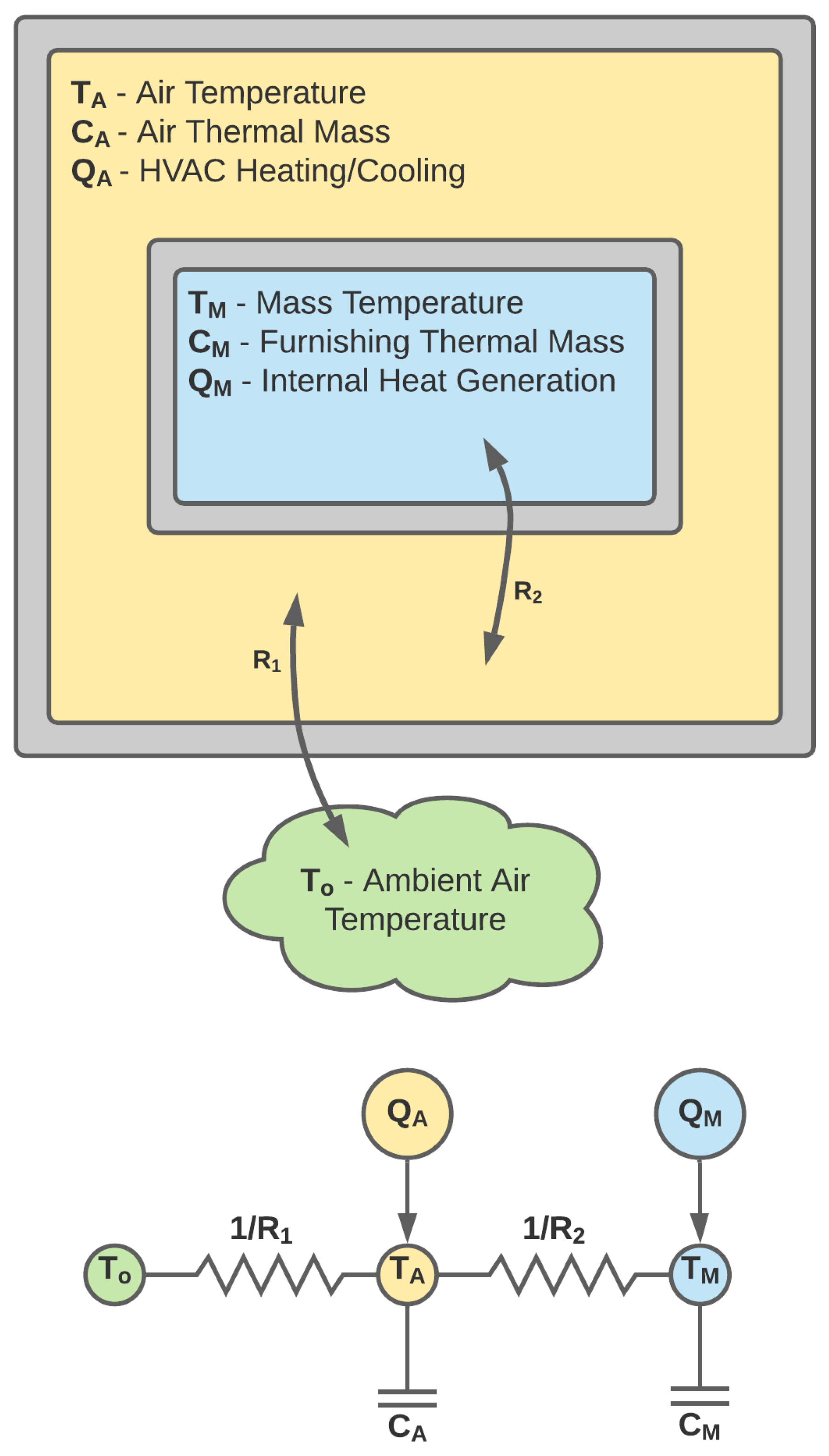
This paper uses the well-established second-order equivalent thermal parameter (EPT) model to describe the temperature dynamics of a residential home. By means of the thermal circuit shown in Figure 1, two coupled first order differential Equations are formed.
and,
where and denote the interior air and lumped mass temperatures of a residential home. Adjacent to the residential control volume is the surrounding outside air temperature . With regard to control theory, both the outside temperature and the internal heat generating elements, denoted , represent disturbances to this thermal system. Rejection of such disturbances is accomplished via the home’s HVAC system, denoted . In particular, represents heat being removed from the interior air. The elegance of this ETP model is that it is fully defined by four measurable parameters, that being the thermal capacities , and the conductive properties , . As will be further discussed in Section 2.4, a parameter estimation model will be presented, which provides systematic method to estimate these thermal parameters.
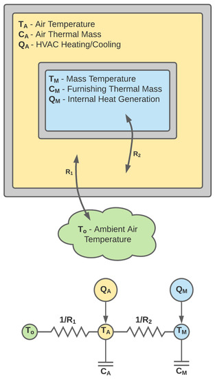
Figure 1.
Second-order equivalent thermal parameter circuit diagram.
Through the manipulation of Equations (1) and (2) a second-order differential equation is formed in terms of and its derivatives and ,
Within Equation (3), the terms and are replaced with and respectively. The negative constant term represents the heat removal capacity of the homes HVAC system and m, a controllable parameter, scales according to the governing control algorithm. , similar to that of , represents alternative heat sources/sinks. In a typical residential setting, includes, but is not limited to, heat generated by home appliances, solar radiation, and the dissipation of heat between the home’s lumped mass and ground. Based on the minimal effects of , especially with regard to , its inclusion will be neglected in this study.
Equation (3) is further abbreviated by replacing each constant term with elements of a parameter vector .
For the sake of clarity, a VSHP regulates the indoor air temperature, , by adjusting its cooling capacity, m, between being fully on or completely off. This range of values may be mathematically defined as the continuous set . A goal of this research is the development of a controller which provides certain beneficial characteristics to an electric utility service provider. These characteristics are the minimization of aggregate power consumption, defined as
and the instantaneous rate of change of aggregate power consumption, . Along with the aggregate power design constraints, this controller must also maintain indoor air temperatures at, or near, its associated set-point temperature . To satisfy the combination of these three control requirements, a novel approach is taken. Instead of directly controlling the cooling capacity of a VSHP by means of its control variable m, this study opts to additionally control its derivative . To distinguish as a controllable parameter, moving forward we redefine it as . A faithful state space representation of Equation (4), incorporating this novel control approach, is defined as follows,
where and,
Through the application of backward Euler method, Equation (6) is therefore rewritten in a discrete format as,
where and k denote the step-length and simulation time-step respectively.
2.2. Decentralized Network Communication
Much of the proposed literature in smart grid systems, particularly TCLs, are constructed using a centralized framework. In such a framework, a utility service provider determines the control action of a population of TCLs, typically by means of tracking an aggregate reference signal. This methodology, including other centralized controllers, have shown great performance benefits. However, there are several glaring drawbacks to a centralized framework. Some of the more prominent challenges include its scalability, vulnerability to cyber-attack, and inherent lack of consumer privacy. To address these challenges, a decentralized framework is introduced in this paper. A decentralized framework relies on the autonomy of participating agent/device to calculate their own control action. As will be demonstrated, the performance of a decentralized controller is further improved through the localized communication between neighboring TCLs.
To address the privacy concerns of participating end-users, communication between VSHPs is limited to what might be ascertained if one were to open their window and listen to when a neighbor’s compressor is cycled off/on. For this reason, each VSHP can only communicate with four other neighboring VSHPs. As a result of this communication, a VSHP’s control action m is partially influenced by the previous control actions of its neighbor set , where is the set of all VSHPs connected to the agent. The entire population set is similarly defined as , which is the set all homes in the given population, .
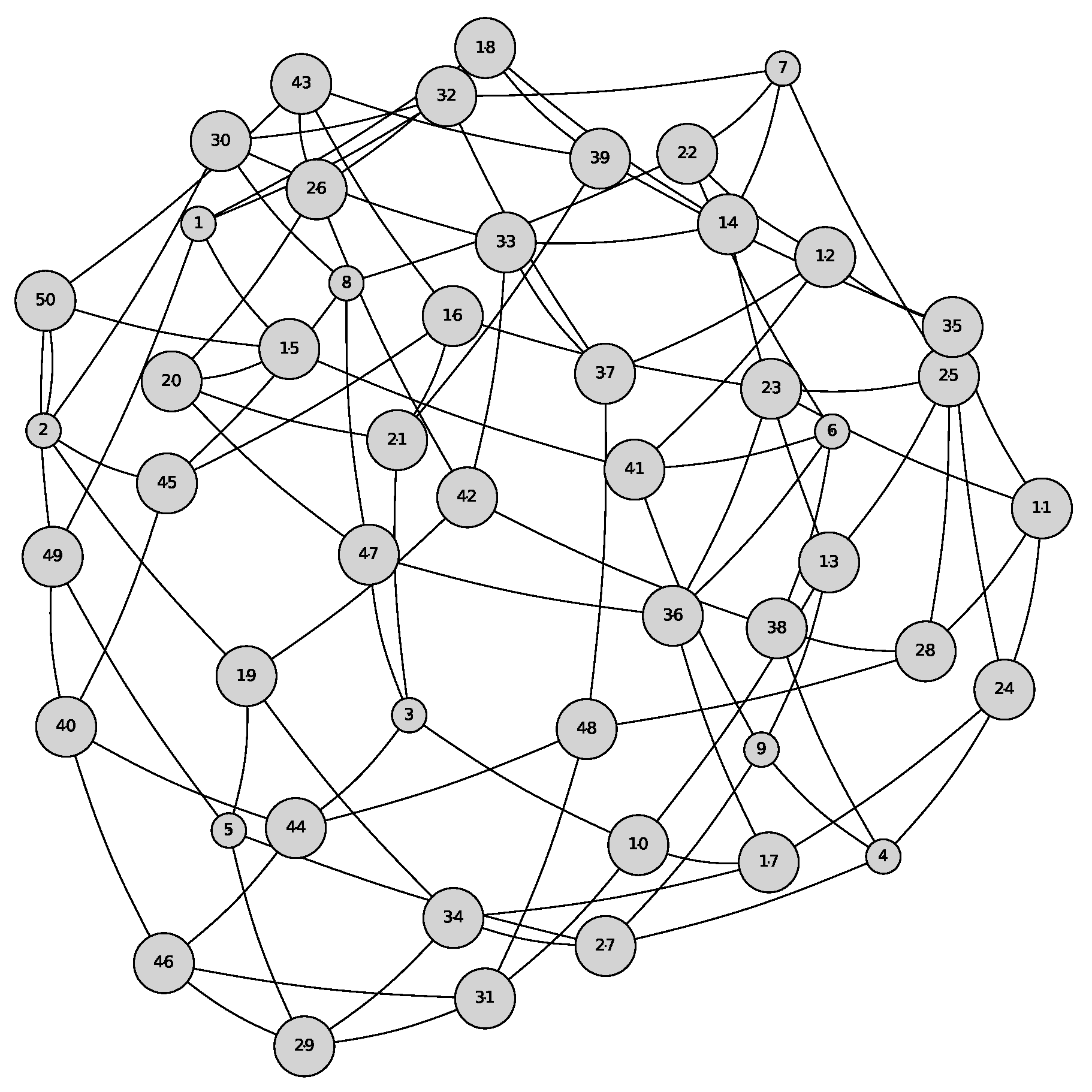
Conventionally, communication is modeled via the elements of an adjacency matrix, . The entry of is nonzero if node i can communicate with node j. Based on the communication constraints proposed above, a random regular graph with a connection degree , such as the one shown in Figure 2, is used to simulate a population of VSHPs.

Figure 2.
Unweighted random regular graph (N = 50, ).
2.3. Demand Response
In addition to the implementation of structured communication, this study also observes the effects of a demand-response event on the proposed controller(s) defined Section 3. A demand-response event, also referred to as a conservation event, is a circumstance where power consumption is systematically controlled by the electric utility to maintain both power generating equipment and the means of distribution within safe operating conditions. Many types of demand-response events exist ranging from emergency protocol to adaptive price control and other related ancillary services. Correspondingly, this study implements the following demand-response event in an effort to test the governing controller with strenuous and unpredictable conditions. Over the time-span , centered about the warmest outside temperature peak , all VSHPs are prevented from conditioning their associated home. This demand-response event, aside from long-term power outages, represents a worst-case scenario regarding aggregate power consumption. During this demand-response event indoor air temperatures will no doubt rise. Upon reinstatement of power, all VSHPs will independently begin cooling their respective homes resulting in a characteristically large spikes in aggregate power consumption.
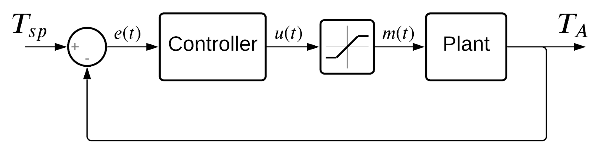
To prime the readers of the challenges associated with this demand-response event, a population of VSHP’s are simulated, whose control action, m, is governed by a typical proportional-integral-derivative (PID) controller. This PID controller represents what would likely be used to regulate a population of independently operated VSHP devices. With the system diagram of Figure 3, in conjunction with the controller defined by Equation (8), a sample population of VSHPs are simulated. The results of this simulation are graphically presented as the subplots of Figure 4. As previously mentioned, a spike in aggregate power consumption is observed. This spike in aggregate power consumption is further reduced at the expense of a larger temperature deviation from the customers set-point preference. The gains of the PID controller in Equation (8) are judicially selected to balance each home’s indoor temperature and the aggregate power of the population. This means that we performed an empirical optimization of the PID gains such that the temperature and power response of the system is the best that we could achieve. This study aims to find a more optimal solution which minimizes spikes in aggregate power consumption while simultaneously maintaining home temperatures at or near their associated temperature set-point, .
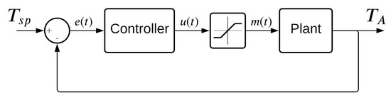
Figure 3.
Closed-loop controller for variable speed heat pump.
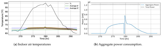
Figure 4.
Population of VSHPs simulated via the PID control framework of Figure 3 (N = 1000, , , and ).
As depicted in Figure 3, a control action , is determined based on the closed loop error signal prior to being constrained via the saturation limits of the maximum cooling capacity, .
2.4. Parameter Estimation
With regard to a physical setting, the thermal parameters , , , and , which define the ETP model, are likely to be measured with some statistical error. Given the proposed ETP model is capable of accurately predicting the dynamics of a residential home, these measurement errors will, by deduction, result in suboptimal controller performance. To account for these initial measurement errors, including other errors that might arise, a recursive least squares (RLS) algorithm is employed to systematically update the thermal parameter vector . Using similar notation presented in [22], an RLS algorithm is constructed by first redefining Equation (4) as,
where the control input, , and regressor, , terms are respectively defined as,
Whether physically measured, or in the case of this simulation, generated about a known statistical distribution, all elements within the parameter vector must be known prior to running the RLS algorithm.
Before the RLS algorithm can predict thermal parameters with sufficient accuracy, both control input and regressor terms are to be collected over the set of initial time-steps to form the following control input and regressor matrices,
The last time-step, , is chosen such that is non-singular. Given the starting value and the adequately populated control input and regressor matrices, which are used to form the inverse covariance matrix, , the RLS algorithm has the following sequence of events,
Within Algorithm 1, denotes the exponential forgetting factor. Unlike the sustained plant dynamics of this study, the thermal properties of a residential home are expected to change over time. The inclusion of this forgetting factor allows for long-term adaptation to the present dynamics. It should be noted, as the RLS algorithm with exponential forgetting becomes the vanilla RLS algorithm. Like many other feedback systems, rejection of system level noise is an important step to achieve stable and robust performance. A low-pass filter is applied, via software, to the newly estimated thermal parameters therefore damping system level noise.
| Algorithm 1. RLS with Exponential Forgetting. |
|
3. Controller
The culmination of this research is the development of a decentralized controller, and to a lesser extent, centralized controller for a population of VSHPs. In brief, two frameworks are presented in Section 3.1 and Section 3.2, which optimally schedule the control actions of a population of VSHPs by means of model predictive control (MPC). As shown in Figure 5, an MPC solves for the control action(s) such that the model dynamics are satisfied and the objective penalty is minimized. Next, the first control action is therefore sent to the VSHP device. Assuming the system’s response is observable, the measured/predicted states are returned to the controller serving as the initial conditions for the following iteration. This sequence is then repeated until a termination condition is met.
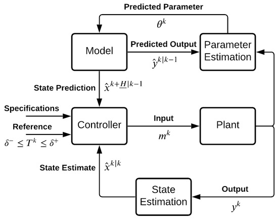
Figure 5.
MPC architecture with parameter estimation.
Two indices are used in Section 3.1 and Section 3.2 to denote time, that being k and . Of the two indices, k denotes the current time-step of the simulation, while represents the step(s) of the controllers predicted horizon which symbolically begins at the index.
3.1. Decentralized Controller (Dc)
In this section, a decentralized controller is developed, whose control action, m, is partially influenced by control actions of its neighbor set . The controller depicted in Figure 5 is mathematically defined as the following quadratic optimization program,
This optimization program minimizes the objective function, , with respect to the state, , and control, m and , decision variables. Through the manipulation of these decision variables, a horizon of control actions are calculated such that the model dynamics, initial conditions, and saturation limits are upheld. To ensure continuity between time-steps, an equality constraint is placed between the initial state values, , and the measured/predicted response of the plant, . Likewise, m is constrained between zero and one, therefore preserving its associated VSHP devices within safe operating conditions. Lastly, the model dynamics of Equation (7), is expressed as a set of linear equality constraints, where the function is defined as,
As shown in Equation (13), the objective function, , is the summation of each time-step’s cumulative objective penalty, , defined as,
Each penalty term of Equation (15) is dedicated to a certain attribute of the desired response. Based the preferences of an electric utility service provider and its end-users alike, this controller must maintain indoor air temperatures while simultaneously minimizing the aggregate power consumption signal and its associated volatility.
The first objective penalty term,
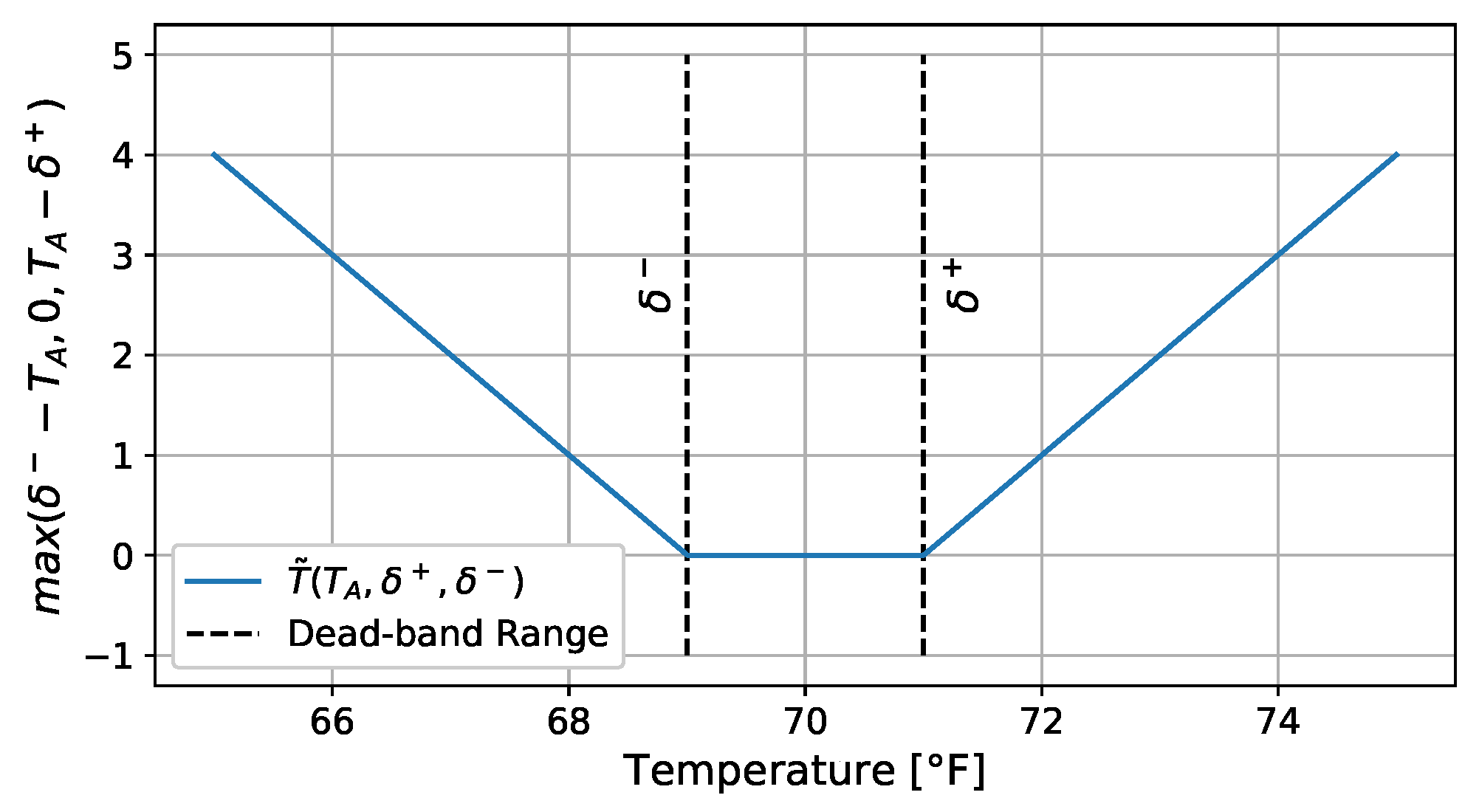
provides a means for optimizer to group aggregate effects via peer-to-peer (P2P) communication. This is done so by minimizing the difference in control action, m, between the agent and its neighbor set . In an effort to reduce aggregate power consumption, defined by Equation (5), individual power consumption is minimized with the penalty term . In addition, a home’s indoor air temperature, , is maintained at or near its set-point temperature, , via the soft constraint . As depicted in Figure 6, the double hinge function, , is mathematically expressed as,
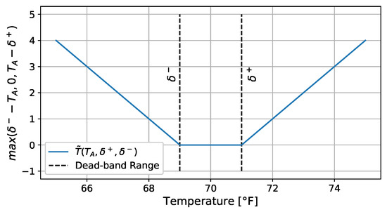
Figure 6.
Objective soft constraint calculated using double hinge function.
If the indoor air temperature, , deviates above or below , a proportional cost will be accrued. Similarly, the minimization of the penalty term, , reduces the rate at which temperature changes in the resulting simulation. Lastly, to ensure the ramp-rate of aggregate power consumption is maintained, the penalty term, , is minimized. This term results in a smoothing effect in aggregate power consumption.
Each of the five objective penalty terms are accompanied by a real numbered objective constant, that being , , , , and . Much like knobs on a dial, these objective constants scale their respective objective penalty term. The qualitative performance of the controller is determined by the relative scale of each objective parameter regarding one another. By deduction, said performance may be tuned in accordance to the attributes described above.
3.2. Centralized Controller (Cc)
Much like the decentralized controller defined above, the preceding centralized controller uses a similarly structured optimization program to determine the control actions of a population of VSHPs. However, unlike the decentralized controller, this centralized controller has omniscient knowledge of the states and control actions of its population. Furthermore, during simulation, this optimization program simultaneously solves for the control actions for an entire population set. In this formulation, the notion of network communication is less meaningful as all information is distributed to and from the electric utility service provider, much like a star graph. This quadratic optimization program has the form,
where and are defined as the collection of all state and control decision variables at the time-step. As may become apparent, the number of decision variables is now directly proportional to the size of the population being simulated. Due to this increased number of decision variables, the associated complexity of the controller so to rises.
The dynamic model is simulated with a set of equality constraints between the incremented state values and the function . Similar to of Equation (14), is now an expressed function of the home, for brevity, its redefinition is omitted. Furthermore, the objective penalty function, , which is summed over each time-step , has the form,
The last four objective penalty terms of Equation (18), are similar to that of Equation (15). However, the penalty term,
is used to minimize the difference in aggregate control effort between adjacent time-step. Observably, this penalty term smooths aggregate power consumption among VSHP devices. Because Equations (16) and (19) focus on the grouping of control actions, they both are scaled the objective constant . The other objective constants , , , and scale their associated objective penalty term.
4. Case Study
HVAC units are typically sold in half ton increments, where one ton of cooling is defined as the amount of heat required to freeze/melt 2000 pounds of water in a 24-h period. Prior to installing a VSHP, the discrete tonnage is chosen according to thermodynamic properties of the space required to condition. Similar to how a residential HVAC system is chosen, in this study a VSHP’s cooling capacity, , is determined based on the time required to cool that home’s indoor air temperature, , from the upper dead-band, , to the lower dead-band, . To assure population heterogeneity, the thermal parameters , , , and are generated about a known statistical distribution. This Gaussian distribution is defined by the mean and standard deviation values listed in Table A1. All other simulation parameters, including objective constants, are therefore listed in Table A2.
As previously stated, and its derivative represent a disturbance to the thermal system. The proposed controllers, shown in Section 3, use a receding horizon approach to determine control action, m, for a corresponding VSHP. This receding horizon controller necessarily requires that and be known prior to simulation. Based on modern metrological forecasting techniques, it is reasonable to assume this outside temperature data are known over the current finite simulation horizon . Conversely, in a simulated environment, like the one presented in this paper, outside temperature data are queued from the National Solar Radiation Database (NSRDB) in the form of a Typical Meteorological Year (TMY) [23]. This TMY dataset, among other qualitative properties, provides hourly ambient outside temperature data. As the name suggests, this dataset represents the most usual weather conditions for a given region and is well suited for the application of weather prediction.
The simulation results generated via Algorithms 2 and 3 are compared using several quantitative metrics. These performance metrics provide a key insight into the load-shedding capability of each control framework. The first two metric, denoted and , describe the peak power drawn before and after the simulated demand response event. Each term is expressed as a ratio between the peak power demand and the total consumable power within the system. For clarity, the total consumable power is the amount of power demanded, assuming all VSHPs operate at full capacity, i.e., . The next performance metric is a measurement of the total energy associated with the aggregate power consumption signals observed in Figure 7b and Figure 8b. In the context of this paper the energy consumed is defined as,
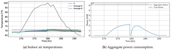
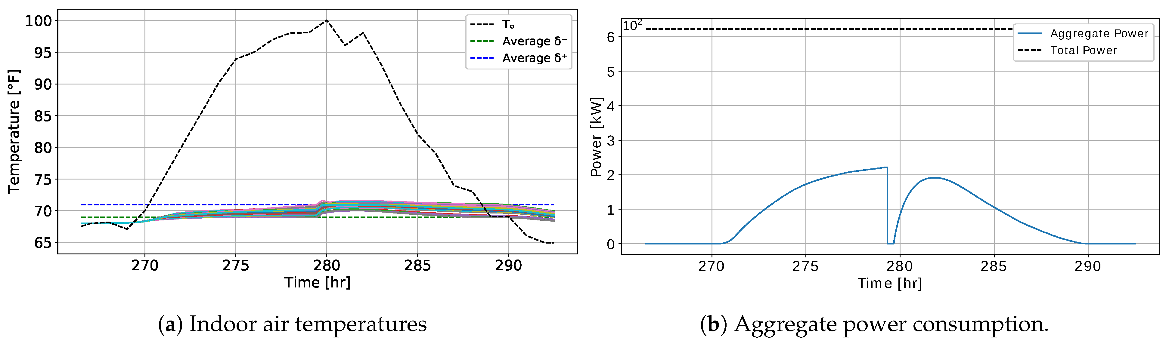
Figure 7.
Decentralized framework simulated via Algorithm 2, (N = 50).
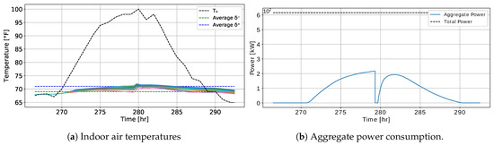
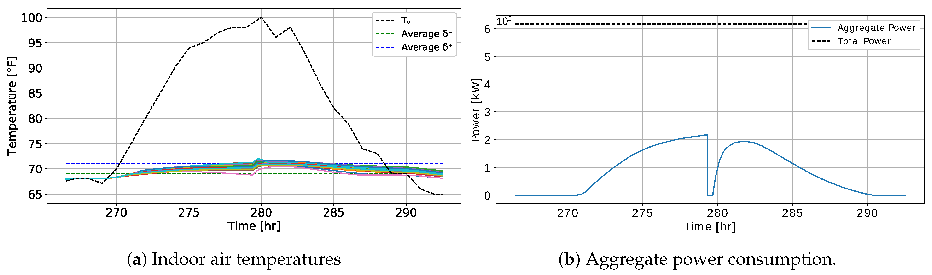
Figure 8.
Centralized framework simulated via Algorithm 3, (N = 50).
To ensure this consumed energy is intrinsically represented, it too is expressed, in Table 1, as a ratio by dividing it with the total consumable energy within the system. As a point of reference, the standard PID controller, shown in Figure 4, is also compared using the three performance metrics described above.
| Algorithm 2. Decentralized MPC Sequence. |
| Initialize |
| Generate |
| Set Initial Conditions |
| for to K do |
| for to N do |

Table 1.
Simulation results.
| Algorithm 3. Centralized MPC Sequence. |
| Initialize |
| Generate |
| Set Initial Conditions |
| for to K do |
Based on the simulation results of Figure 7 and Figure 8, in addition the quantitative metrics listed in Table 1, both control frameworks are observed to similar performance attributes. Unlike the PID controller defined in Section 2.3, both optimal control frameworks reduce the load synchronization effects caused by the demand-response event. Furthermore, Figure 7b and Figure 8b show a smooth gradual increase in aggregate power consumption. This reduction in is partially attributed to the scheduling of control actions accomplished via the minimization the objective penalty terms (16) and (19). For the other quantitative metrics, and , little change is observed between control frameworks.
A key difference between the centralized and decentralized controllers defined in Section 3, is the computational complexity associated with each framework. For the centralized controller, the number of decision variables within the optimization program of Equation (17) is directly proportional to the number of homes being simulated, N. As the number of simulated homes increases, so too increases the time required to compute the population of control actions, assuming all auxiliary features remain constant. An advantageous feature of the decentralized framework is that the computational complexity required to solve a control action for a VSHP remains constant. This assertion is exemplified by the simulation runtimes listed in Table 2. The proposed decentralized controller necessarily requires that each VSHP compute its own control action.
Table 2.
Resultant Simulation times.
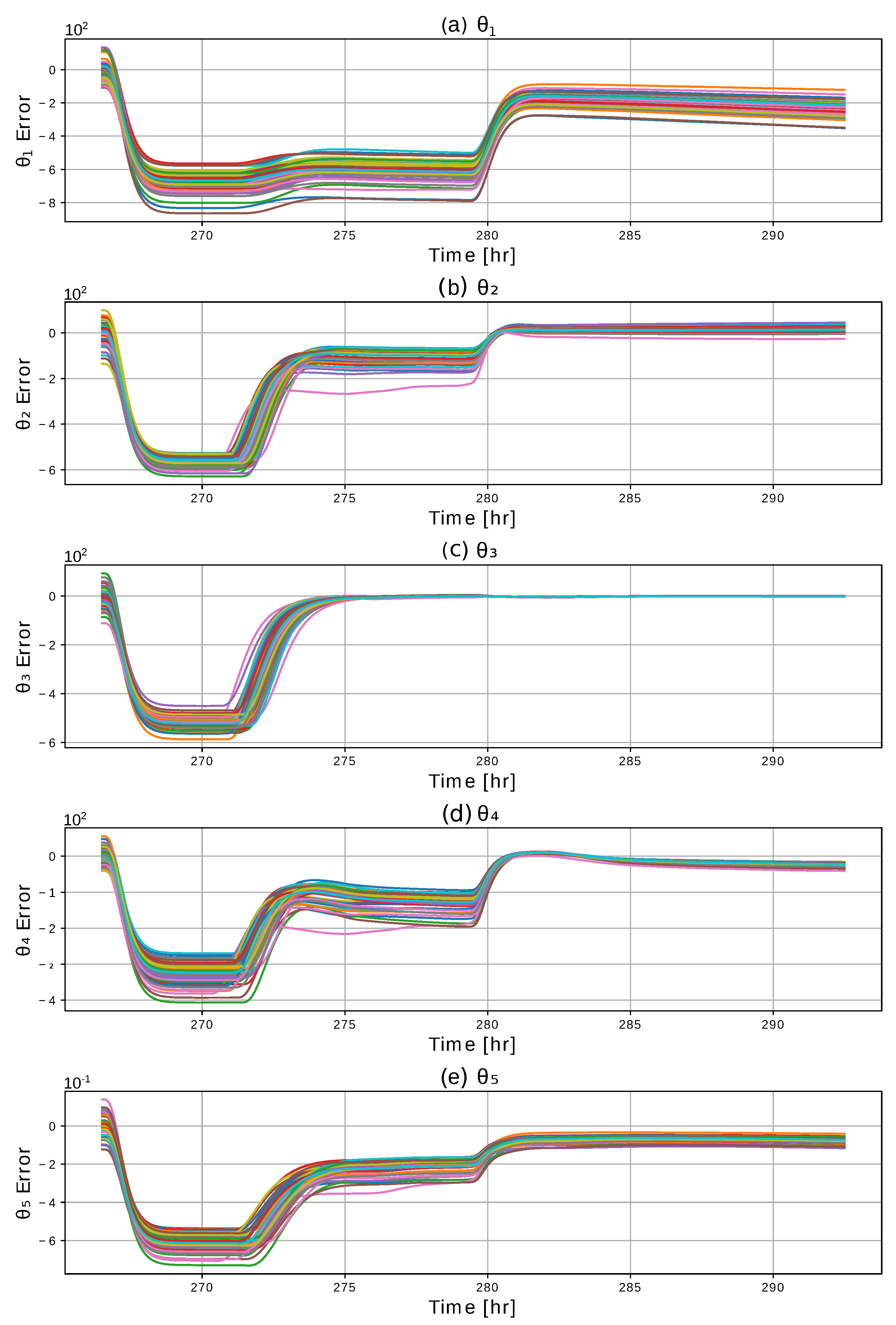
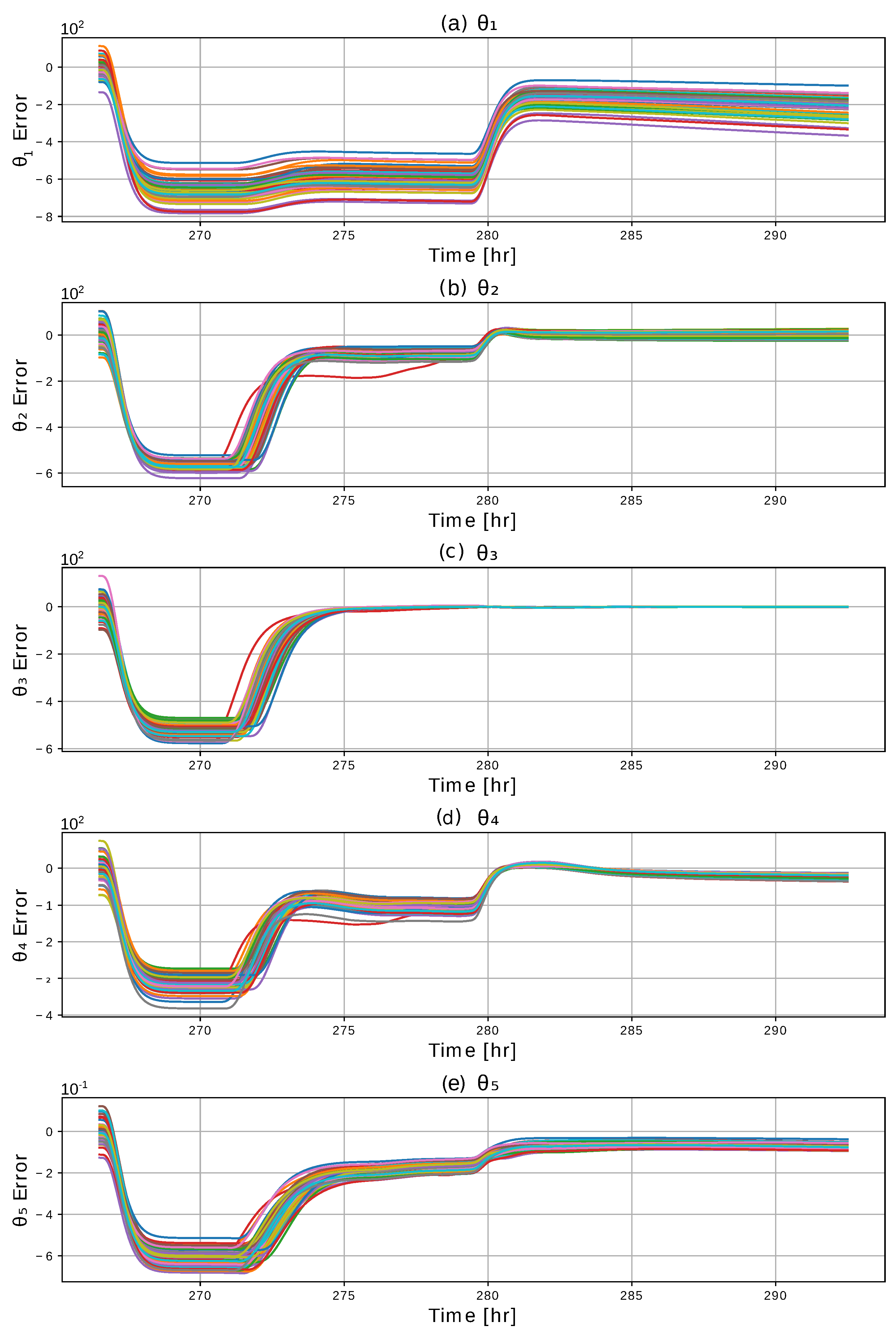
By way of Algorithm 1, elements of the thermal parameter vector, , are systematically updated to improve the accuracy and resilience of the predictive model. These incremental updates provide an ETP model the wherewithal to accurately mimic the dynamics of its respective plant. To show convergence between the model and plant dynamics an error signal is generated for each element of the thermal parameter vector. This error signal is defined as the difference between the plant and model parameter values, i.e., . Each error signal is graphically depicted by the subplots of Figure 9 and Figure 10. Due to its initialization process, these thermal parameters show a tendency to deviate from the plant values during early time-steps of the simulation. We also observe that before the demand-response event, these thermal parameters tend not to converge upon their respective plant value. This failure to converge is partially attributed to the lack of persistence of excitation. After the demand-response event, parameters then converge upon their desired plant value. In a real setting, the true thermal parameters of the proposed ETP model, which defines the plant dynamics, are likely uncharacterizable by a linear approximation. Moreover, it is reasonable to assume the thermal characteristics of a home are capable of change by way of renovation or degradation. For these reasons, two update condition are employed to help determine periods of stable prediction. The first update condition is , where is the condition number of , as defined in Algorithm 1, and is an empirically determined constant. In Figure 9 and Figure 10, it may be observed that the system parameters change rapidly during the initial stages of the system response. This may be attributed to the condition number being relatively large. The second indicator used to predict convergence is the rate at which each thermal parameter varies. Thermal parameters are therefore updated when the condition, , holds. similar to the value of , the value of is empirically determined. The combination of these two conditions attempts to predict when the thermal parameters are capable of being updated. Each thermal parameter must be initialized within an approximate region of the true parameter characteristics.
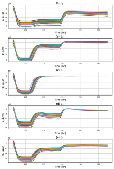
Figure 9.
Thermal parameters of the decentralized framework updated via Algorithm 1, (N = 50).
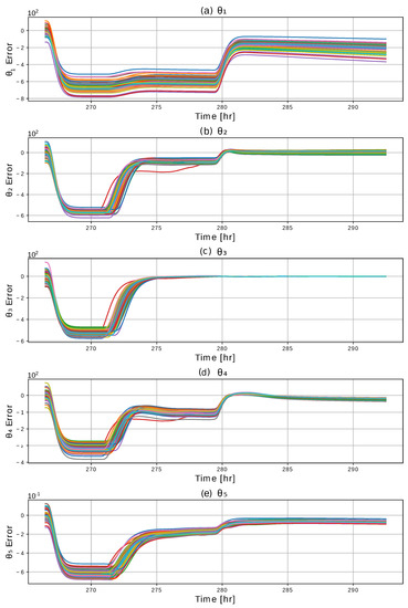
Figure 10.
Thermal parameters of the centralized framework updated via Algorithm 1, (N = 50).
Remark 1.
It is a standard result of adaptive control theory that when the inputs to a control system do not excite sufficient modes of the system, parameter estimation does not converge to their correct values. For a detailed exposure, the reader is invited to see Chapter 2.4 (page 63) of [22].
5. Conclusions
In this paper, we develop a decentralized control framework to optimally schedule the control actions of a population of VSHPs. Albeit contradictory, this control framework balances end-user temperature requirements with an electric utility service provider’s desire to supply smooth predictable power. We show through minimal network communication that our decentralized control framework performs on par with a similarly structured centralized controller with omniscient knowledge of the state and control actions of its population. Based on the quantitative metrics presented in Section 4, we also show this decentralized control framework alleviates the load aggregations experienced by more traditional PID controllers. In an effort to improve the accuracy of our controller, we implement a recursive least squares algorithm to adaptively update the parameters defining the second-order ETP model. Although failing to converge under certain simulated conditions, this RLS algorithm proved useful in the convergence of parameters when stimulated with a demand response event. Over longer simulated time periods, by means of persistence of excitation, we conclude that thermal parameters will eventually approach a desired value such that the dynamic model mimics the response of the plant. Further experimental validation is needed to show the efficacy of our simulation. Such experiments will be the focus of future research. Due to the approvals needed by local utilities, regulators, and participants alike, significant planning is required to perform the necessary experiments. This research serves as an important precursor to future experimental studies.
Author Contributions
R.S.M.: Formal analysis, Investigation, Data curation, Software, Writing—original draft; J.F.G.: Supervision, Project administration, Investigation, Writing—review & editing; A.C.S.: Supervision, Project administration, Investigation, Formal analysis, Software, Writing—review & editing. All authors have read and agreed to the published version of the manuscript.
Funding
This work was supported in part by the US Department of Energy, DOE-EE0007726 and the Center for Advanced Energy Studies at Boise State University.
Institutional Review Board Statement
Not applicable.
Informed Consent Statement
Not applicable.
Conflicts of Interest
The authors declare no conflict of interest.
Appendix A
Table A1.
Gaussian distribution of thermal parameters.
Table A1.
Gaussian distribution of thermal parameters.
| Thermal Parameter | Mean | Std. |
|---|---|---|
| 1080 | 54 | |
| 4280 | 214 | |
| 520 | 26 | |
| 7050 | 353 |
Table A2.
Simulation parameters of decentralized (DC) and centralized (CC) controllers.
Table A2.
Simulation parameters of decentralized (DC) and centralized (CC) controllers.
| (DC) | (CC) | ||
|---|---|---|---|
| Objective Constants | 200 | 300 | |
| 5000 | 8000 | ||
| 100 | 100 | ||
| 1000 | 1500 | ||
| Simulation Parameters | Homes (N) | 50 | |
| Time-step (K) | 4000 | ||
| Horizon (H) | 20 | ||
| Step-length () | 23.4 [s] | ||
| D.R. length | 20 [min] | ||
References
- Hao, H.; Sanandaji, B.M.; Poolla, K.; Vincent, T.L. A generalized battery model of a collection of thermostatically controlled loads for providing ancillary service. In Proceedings of the 2013 51st Annual Allerton Conference on Communication, Control, and Computing (Allerton), Monticello, IL, USA, 2–4 October 2013; pp. 551–558. [Google Scholar]
- Bacciotti, A. Stability and Control of Linear Systems; Springer: Berlin/Heidelberg, Germany, 2019. [Google Scholar]
- Kuwada, J.; Schwartz, R.; Gardner, J.F. Local communication in populations of thermostatically controlled loads. ASME J. Eng. Sustain. Build. Cit. 2020, 1, 030901. [Google Scholar] [CrossRef]
- Malhame, R.; Chong, C.-Y. Electric load model synthesis by diffusion approximation of a high-order hybrid-state stochastic system. IEEE Trans. Autom. Control 1985, 30, 854–860. [Google Scholar] [CrossRef]
- Callaway, D.S. Tapping the energy storage potential in electric loads to deliver load following and regulation, with application to wind energy. Energy Convers. Manag. 2009, 50, 1389–1400. [Google Scholar] [CrossRef] [Green Version]
- Zhang, W.; Lian, J.; Chang, C.-Y.; Kalsi, K. Aggregated modeling and control of air conditioning loads for demand response. IEEE Trans. Power Syst. 2013, 28, 4655–4664. [Google Scholar] [CrossRef]
- Koch, S.; Mathieu, J.L.; Callaway, D.S. Modeling and control of aggregated heterogeneous thermostatically controlled loads for ancillary services. In Proceedings of the 17th Power Systems Computation Conference, PSCC, Stockholm, Sweden, 22–26 August 2011; pp. 1–7. [Google Scholar]
- Liu, M.; Shi, Y. Model predictive control of aggregated heterogeneous second-order thermostatically controlled loads for ancillary services. IEEE Trans. Power Syst. 2015, 31, 1963–1971. [Google Scholar] [CrossRef]
- Zhou, Y.; Wang, C.; Wu, J.; Wang, J.; Cheng, M.; Li, G. Optimal scheduling of aggregated thermostatically controlled loads with renewable generation in the intraday electricity market. Appl. Energy 2017, 188, 456–465. [Google Scholar] [CrossRef]
- Chen, B.; Yao, W.; Francis, J.; Berges, M. Learning a distributed control scheme for demand flexibility in thermostatically controlled loads. arXiv 2020, arXiv:2007.00791. [Google Scholar]
- Ruelens, F.; Claessens, B.J.; Vandael, S.; Schutter, B.D.; Babuška, R.; Belmans, R. Residential demand response of thermostatically controlled loads using batch reinforcement learning. IEEE Trans. Smart Grid 2016, 8, 2149–2159. [Google Scholar] [CrossRef] [Green Version]
- Ruelens, F.; Claessens, B.J.; Vrancx, P.; Spiessens, F.; Deconinck, G. Direct load control of thermostatically controlled loads based on sparse observations using deep reinforcement learning. Csee J. Power Energy Syst. 2019, 5, 423–432. [Google Scholar]
- Kazmi, H.; Suykens, J.; Balint, A.; Driesen, J. Multi-agent reinforcement learning for modeling and control of thermostatically controlled loads. Appl. Energy 2019, 238, 1022–1035. [Google Scholar] [CrossRef]
- Hao, H.; Sanandaji, B.M.; Poolla, K.; Vincent, T.L. Aggregate flexibility of thermostatically controlled loads. IEEE Trans. Power Syst. 2014, 30, 189–198. [Google Scholar] [CrossRef]
- Chassin, D.P.; Stoustrup, J.; Agathoklis, P.; Djilali, N. A new thermostat for real-time price demand response: Cost, comfort and energy impacts of discrete-time control without deadband. Appl. Energy 2015, 155, 816–825. [Google Scholar] [CrossRef] [Green Version]
- Ruth, M.; Pratt, A.; Lunacek, M.; Mittal, S.; Wu, H.; Jones, W. Effects of Home Energy Management Systems on Distribution Utilities and Feeders under Various Market Structures; Technol Report; National Renewable Energy Lab. (NREL): Golden, CO, USA, 2015.
- Hull, J.; Khurana, H.; Markham, T.; Staggs, K. Staying in control: Cybersecurity and the modern electric grid. IEEE Power Energy Mag. 2011, 10, 41–48. [Google Scholar] [CrossRef]
- Kimani, K.; Oduol, V.; Langat, K. Cyber security challenges for iot-based smart grid networks. Int. J. Crit. Infrastruct. Prot. 2019, 25, 36–49. [Google Scholar] [CrossRef]
- Tindemans, S.H.; Trovato, V.; Strbac, G. Decentralized control of thermostatic loads for flexible demand response. IEEE Trans. Control. Syst. Technol. 2015, 23, 1685–1700. [Google Scholar] [CrossRef]
- Wan, Y.; Long, C.; Deng, R.; Wen, G.; Yu, X.; Huang, T. Distributed event-based control for thermostatically controlled loads under hybrid cyber attacks. IEEE Trans. Cybern. 2020. [Google Scholar] [CrossRef] [PubMed]
- Kuwada, J.; Mehrpouyan, H.; Gardner, J.F. Design resilience of demand response systems utilizing locally communicating thermostatically controlled loads, In ASME International Mechanical Engineering Congress and Exposition; American Society of Mechanical Engineers: New York, NY, USA, 2019; Volume 59438, p. V006T06A045. [Google Scholar]
- Aström, K.J.; Wittenmark, B. Adaptive Control; Courier Corporation: Chelmsford, MA, USA, 2013. [Google Scholar]
- Sengupta, M.; Xie, Y.; Lopez, A.; Habte, A.; Maclaurin, G.; Shelby, J. The national solar radiation data base (nsrdb). Renew. Sustain. Energy Rev. 2018, 89, 51–60. [Google Scholar] [CrossRef]


Publisher’s Note: MDPI stays neutral with regard to jurisdictional claims in published maps and institutional affiliations. |
© 2021 by the authors. Licensee MDPI, Basel, Switzerland. This article is an open access article distributed under the terms and conditions of the Creative Commons Attribution (CC BY) license (https://creativecommons.org/licenses/by/4.0/).