Abstract
In this work, the problematic identification of the main sources of noise occurring from the exploitation of railway vehicles moving at a speed of 200 km/h were analyzed. Within the conducted experimental research, the testing fields were appointed, measurement apparatus selected, and a methodology for conducting measurements was defined, including the assessment of noise on a curve and straight track for electric multiple units of the so-called Pendolino, an Alstom type ETR610 series ED25 train. The measurements were made using a microphone camera Bionic S-112 at a distance of 22 m from the track axis. As a result of the conducted experimental research, it was indicated that the noise resulting from vibrations arising at the wheel-rail contact (rolling noise) was the dominant source of sound.
1. Introduction
Due to the continuous modernization of railway lines aimed at increasing the operating speed of vehicles, as well as the systematic approach of acoustically protected buildings to railway areas, the noise threat is increasing. Noise has for many years become the main source of pollution from rail transport; therefore, its effects are experienced by an increasing number of people. There are many ways of limiting and reducing noise in rail transport, including constructional solutions used in railway vehicles as well as methods used on railway lines to preserve acoustically protected areas. In order to effectively select and apply solutions and methods to reduce the negative impact of noise on the environment, it is necessary to properly and thoroughly identify the acoustic emission of railway vehicles, including among others. the main sources of noise emissions [1,2,3,4,5].
It is worth mentioning that the occurrence of noise, or acoustic emission, can also bring many benefits. Acoustic emission analysis is used in many sectors of transport and industry, among others, to detect and monitor damages, leaks, fatigue, or structural analysis of various materials (e.g., concrete, plastics, wood, ceramics) [6,7,8,9,10,11,12].
The aim of this paper is to present the results and conclusions of an experimental study using an acoustic camera. The research was conducted in order to identify the main sources of noise coming from vehicles with an operating speed of 200 km/h.
Currently, on the railway lines in Poland, Alstom company vehicles type ETR610 series ED250 (the so-called Pendolino) can move at such a speed. There is a great need to analyze the dominant sources of noise from high-speed railway vehicles and to determine unambiguously whether, at speeds of about 200 km/h, the main contributors are rolling noise or aerodynamic noise [13,14,15]. Identifying the dominant sources of noise from Alstom’s ETR610 series ED250 vehicles will enable a more effective selection of noise mitigation solutions. A block diagram of the tests carried with the use of an acoustic camera is shown in Figure 1.
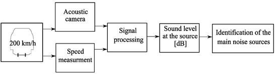
Figure 1.
A block diagram of the tests carried with the use of an acoustic camera.
The topic of identification of the main sources of noise from railway vehicles has been addressed by many authors [15,16,17,18,19,20]; however, studies included measurements of vehicles moving at speeds above 200 km/h. The analysis of the available literature did not reveal detailed measurements carried out on Alstom ETR610 series ED250 vehicles traveling at speeds of 200 km/h.
Conducted measurements with the use of an acoustic camera were one of the three stages of the conducted tests. In the course of the research, the following actions were also performed:
- Measuring of the sound level in the measurement cross-section with the use of the 2 × 4 microphone array (four measurement points at the distance of 5 m, 10 m, 20 m, 40 m from the track axis, and two microphones each at the height of the railhead and 4 m from the railhead);
- Measurements of track and sub-track vibrations.
The experimental tests were to enable obtaining the acoustic signature of the examined vehicle by:
- Identification of the main sources of noise;
- Obtaining time history, recorded for each train passage separately, with a step of 1 s, containing the average sound level LAeq 1s, as well as obtaining the frequency spectrum of noise ranging from 20 Hz to 20 kHz, with bands divided into thirds;
- Obtaining the vibration propagation pattern in the nearest surroundings of the railway line (track and sub-track);
- Obtaining the vibrations propagation scheme in the nearest surrounding of the railway line (track and substructure).
The methodology of the conducted experimental research is shown in the following block diagram (Figure 2).
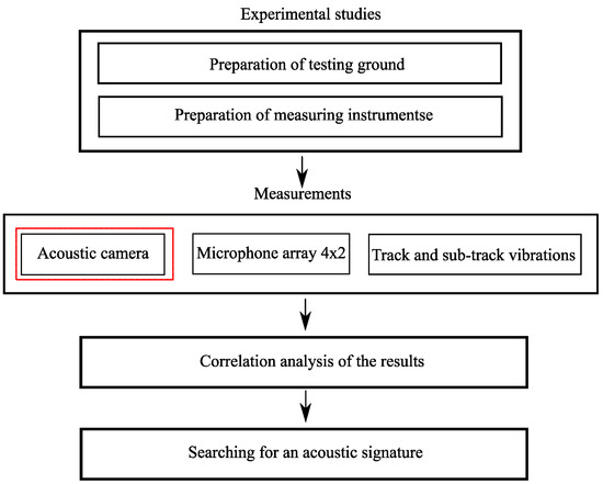
Figure 2.
The Block diagram of the methodology of the conducted experimental research.
2. Materials and Methods
2.1. Technical Specification of the Alstom Composite Trainsets, Type ETR610—ED250 Series—Pendolino
The object of experimental research was an Alstom composite traction unit type ETR610—series ED250—Pendolino (Figure 3). These vehicles are managed by the biggest carrier in Poland—PKP Intercity S.A. Pendolino vehicles are bi-directional electric multiple units consisting of seven units, including four engine units (two outboard on both sides) and three outboard (middle) units [20].
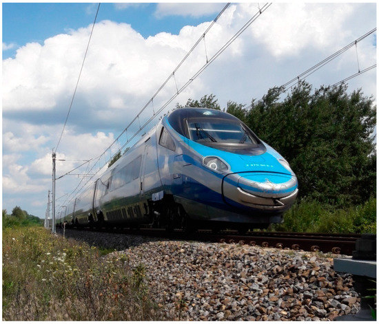
Figure 3.
Research object: Alstom vehicle ETR610—ED250 series—Pendolino.
Standard gauge vehicles (adapted for 1435 mm gauge track) are equipped with 8 traction motors, asynchronous, three-phase with a power of 708 kW each. The train is suitable for passenger service at stations with a platform height of 760 mm and 550 mm above the railhead, as well as at lower platforms up to a height of 250 mm with the use of a special step. The basic technical parameters of the test object are shown in Table 1.

Table 1.
Basic technical parameters of the ETR610 vehicle—ED250 series—Pendolino [20,21,22].
In Pendolino vehicles, the drive and engine are located entirely under the car bodies. All the power is transmitted to the wheelset by means of a Cardan articulated shaft and an axial bevel gear. Appropriate dynamic characteristics of the vehicle on curves at speeds of 250 km/h are ensured by two-axle bogies equipped with steering dampers. The bogies have one drive axle and one rolling axle with very low weight. The bogie frame is a steel construction, while the train bodies are made of aluminum profiles [20,21].
The vehicle was equipped with two braking systems: pneumatic (steel discs and sintered pads) and an electromagnetic rail brake. The average acceleration of the vehicle on a horizontal straight section is equal to 0.36 m/s2 [20].
2.2. Railway Track Tested
For experimental research, we chose two sections (a straight section and a curve) of the railway line No. 4 Grodzisk Mazowiecki–Zawiercie, on the section Grodzisk Mazowiecki–Idzikowice. Detailed information on the location of measurement cross-sections is presented in Section 2.3. Below, basic construction parameters of the railway line, on which acoustic measurements were conducted, and the area around measurement cross-sections were characterized. In Figure 4, the experimental research area on the curved railway line at km 18 + 600 is presented.
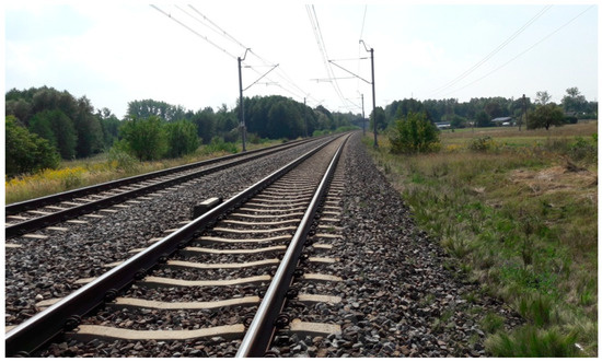
Figure 4.
Railway track at km 18 + 600—experimental research area (curve).
According to the manual [23,24], the railway line in question is a main line, electrified, and mostly double track. It is built with UIC60 contactless rails, on pre-stressed concrete sleepers with the SB fastening system, laid on a ballast bed. The general technical condition of the railway track on which the measurements were conducted was defined as good.
In the case of the measurement cross-section located at km 18 + 600 (the curve), the area around the measurement site is mainly agricultural with single-family houses (the nearest buildings are situated behind the measurement cross-section at the distance of approximately 15–20 m). The area around the research site located at km 21 + 300 (straight section) is agricultural.
2.3. Location of the Testing Ground
The measurements of acoustic signals were conducted on No. 4 railway Line Grodzisk Mazowiecki–Zawiercie, section Grodzisk Mazowiecki–Idzikowice, at two locations:
- Curve—approximately km 18 + 600 (Świnice, Dluga street);
- Straight section—approximately km 21 + 300 (Szeligi, Dojazdowa street).
2.4. Selection of Measuring Equipment
Measurements of the sound level from high-speed railway vehicles were made using measurement equipment consisting of the following devices:
- Noise Inspector Bionic M-112 acoustic camera;
- Speedmeter;
- Davis Instruments Vantage Pro2 weather station.
2.5. Weather Conditions
The experimental tests were performed on days with favorable meteorological conditions, i.e., no precipitation (rain, snow, and hail) and conditions not exceeding the parameters specified in Annex No. 7 of the regulation [25].
Measurement of atmospheric conditions: wind speed and direction, atmospheric pressure, air temperature, and humidity, was performed using a Davis Instruments Vantage Pro2 weather station located outside the range of the gust from a passing train at the height of about 3.5 m.
2.6. Methodology of Site Measurements
Experimental tests were carried out in 8–9 August 2019 (straight section) and 28–29 August (curve) on railway line No. 4 Grodzisk Mazowiecki–Zawiercie. The measurements were performed on working days (2 days, in each of the measurement cross-sections) during the operating hours of increased speed vehicles, i.e., between 08:00 and 20:00.
Experimental tests were carried out during the passage of Alstom railway vehicles type ETR610—ED250 series—Pendlino on the selected measurement route without stops at a speed of about 200 km/h on a straight section and curve. At a distance of about 22 m from the track axis, the measurement was carried out using a microphone camera Noise Inspector Bionic M-112, with a sampling frequency of 12 Hz. The acoustic camera used during the measurements is shown in Figure 5, whereas in Figure 6, a schematic of the measuring section is presented.

Figure 5.
Microphone camera Noise Inspector Bionic M-112.

Figure 6.
Instrumented cross-section Turing experimental tests.
The extracted, measured values were processed using in-camera software to obtain the noise levels at the object under study (source). In order to determine the sound levels at the source, the following relation was used [25,26]:
where L is the estimated noise level at source; Lzm is the value measured at the receiver (acoustic camera); l is the distance from the noise source (m).
L = Lzm + 20log(l) [dB]
The measurements made it possible to determine the dominant sources of noise generated by high-speed railway vehicles.
The acoustic array used for experimental research, equipped with an optical camera and 112 directional microphones, uses for measurements the method of acoustic holography (from 40 Hz) and beamforming (above 400 Hz), which enables us to obtain results within the range of frequencies up to 24 kHz [27]. For localization of dominant noise sources, the second method was used, which was dedicated to measurements above 1 m from the source. This method processes the spatial-temporal signal recorded by an acoustic camera. Each microphone has an assigned time delay relative to the center of the acoustic matrix, allowing the signal beam to be focused in the direction of acoustic wave propagation [28,29,30,31,32,33]. A simplified diagram of signal analysis by an acoustic camera is shown in Figure 7.

Figure 7.
Simplified diagram of acoustic camera signal analysis.
Time delays assigned to each microphone of the acoustic matrix enable focusing the signal beam in the direction of propagation of an acoustic wave. The signal received by the microphones, delayed by an appropriate time, is summed at the output of the matrix and thus amplified compared to measurements with only one microphone [31,32,33,34,35,36,37,38]. This calculation in the time domain was performed using the following formula [28,35,37]:
where ωn is the weight multiplied on the output signal of the nth microphone; τn is the time delay for each microphone of the matrix; pn is the coordinate of the nth microphone.
In the case of transformation of the above formula in the frequency domain using Fourier’s transform, the resultant signal can be expressed by the formula [31,37]:
where ωT is the output signal of the nth microphone; k is the unit wave vector; Fn is the Fourier‘s transform of the signal of the nth microphone.
Thanks to the use of time delay for individual microphones, the measured signal was the same for the whole microphone matrix. The size of time delays depends on the type of acoustic wave (flat and spherical), which travel differently in respect to the nth microphone and the reference microphone [32,36,37,38]. The acoustic beamforming for a plane wave is shown in Figure 8.
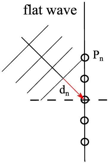
Figure 8.
The acoustic beamforming for a plane wave [28].
Time delay (τn) for a flat wave is determined accordingly to the below formula [31,37,39,40]:
where dn is the difference in distance covered by the wave; pn is the defined position of the nth microphone; a is the unit vector of the incident wave; c is the speed of sound wave propagation.
For a spherical wave occurring in the case of a point source, the magnitude of the time delays is determined by Equation (5) [31,39]:
where r is the distances between the acoustic matrix middle and the point source and l is the distance between the nth microphone source and the point source.
According to the criterion for assessing the harmfulness of noise for the environment, the equivalent sound level should be taken into account. For the steady noise, the average sound level with the correction filter A (LAm) or the equivalent sound level (LAeq) for the observation time is to be determined [41]. It is taken as the eight most unfavorable hours of the day (in the range 6:00 a.m.–10:00 p.m.) or thirty analogous minutes during the night time (in the range of 10:00 p.m.–6:00 a.m.). In the case of transient noise, the A-weighted sound level (LAeq) for the above-mentioned time and the maximum A-sound level (LAmax), taking into account the slow time characteristics. The equivalent sound level, taking into account sound events from a given time interval, can be determined using Equation (6) [42,43]:
where Te is the exposition time; p is the measured value of the sound pressure in Pa; p0 is the reference pressure, set at 20 μPa.
2.7. Intensity and Energy of Sound Waves
The instantaneous value of the acoustic energy density is the sum of the kinetic energy density and the potential energy (Hall, 1987). Energy In the near field, for a short distance from the sound source, the kinetic energy density is much greater than the one of the potential energy, but the condition for energy transfer in space is the conversion of kinetic energy into potential and vice versa. For the far-field, the average values of the kinetic and potential energy densities are equal [44]. The intensity of the acoustic wave is equal to the sound power transmitted by the wave. It can be defined as the average value of the energy flux flowing during 1 s through a unit area of 1 m2, perpendicular to the direction of wave propagation. They can be presented using the following formula in the case of a spherical wave [44,45]:
Since the intensity of an acoustic wave is the product of the average density of its total energy and the speed of sound in air, the total energy in the far-field can be calculated using the following formula [44,45]:
According to the theory, doubling the distance from a sound source means a four-fold decrease in the intensity or energy of the sound, which is important because the area occupancy in the case of railway lines is significant. In the next section, the analyzes of the intensity ranges of the emitted sound waves are presented.
3. Reference to the Normative Values in Force
An important document, in reference to the noise generated by high-speed railway vehicles, is the technical specifications of TSI Noise [46,47], which defines, among others, limit values for the sound levels for stationary noise, starting noise, and pass-by noise. The limit values for electric multiple traction units are shown in Table 2. When determining the average value of the equivalent sound level, for 20 passes, at a distance of 7.5 m from the track, according to the TSI requirements, the values shown in Table 2 were obtained.
Table 2.
Acceptable values of sound levels for the stationary noise, starting noise, and pass-by noise of electric traction units.
For stationary noise, the acceptable values under standard conditions are defined for:
- -
- The equivalent continuous sound level A of the unit (LpAeq,T(unit));
- -
- The equivalent continuous sound level A at the nearest measuring position “i”, including the main air compressor (LipAeq,T).
The starting noise acceptable values for high-speed vehicles for the maximum equivalent continuous sound level with A correction and the FAST time constant (LpAF,max) are set at 80 dB.
For pass-by noise, the maximum acceptable values for the equivalent continuous sound level A for high-speed vehicles at 80 km/h is equal to 80 dB. According to the TSI Noise guidelines, the obtained measurement results were normalized to the reference speed (80 km/h) using Equation (9):
where Vtest is the speed measured during tests.
LpAeq,Tp(80km/h) = LpAeq,Tp(Vtest) − 30 ∗ log (Vtest/80 km/h)
In Poland, the normative values of noise in the environment, which originate from rail transport, are indicated in the Regulation of the Minister of Environment, 14 June 2007, on permissible levels of noise in the environment [47]. The regulation [47] introduces a division of acoustically protected areas, depending on their function and type of development, for which different permissible noise levels have been defined for the daytime (16 h), i.e., during the period of the day from 6:00 to 22:00, and at nighttime (8 h), covering the period from 22:00 to 6:00.
In the first group of acoustically protected areas, there are areas of health-resort protection and areas of hospitals located outside the city. The second group includes single-family housing, housing with a permanent or temporary occupation by children and youth, or seniors care facilities and hospitals in cities. The third group of areas includes multi-family housing and collective residence, homestead development, recreational and leisure areas, and housing and services.
The last group of areas allows the creation of a downtown zone in cities with a population over 100,000, i.e., areas of intensive development in the city-center area as specified in the local spatial development plan with a concentration of service, commercial and administrative facilities.
An excerpt from the annex to the regulation indicating permissible noise levels for individual groups of areas is presented in Table 3.
Table 3.
Classification of protected areas and acceptable values for environmental noise levels expressed as LAeqD and LAeqN indicators for railway lines.
Based on the above guidelines, in this paper, the cumulative impact on the surroundings was analyzed, taking into account the n analyzed frequency bands (i). For this purpose, the total equivalent sound level has been determined using Equation (10):
Taking into consideration a simplified model of noise propagation, instantaneous equivalent sound levels LAeq(r) were determined as a function of distance from the source according to Equation (11), for the distance at which the train is treated as a linear source and in the second case as a point source:
where r0 is the distance of the referential measurement from the noise source and is the equivalent sound level at the reference point.
The following band defining the levels for 20 trains passing by was obtained (Figure 9).

Figure 9.
Sound level distribution according to distance from the source.
4. Results and Discussion
The sound level values achieved during the measurements were transformed according to the relation (1) to obtain the results occurring at the source, i.e., high-speed railway vehicles. This paper presents selected results that were recorded for a straight section and a curve for frequencies from 500 Hz to 3000 Hz (grouped into ranges: 500–1000 Hz, 1000–2000 Hz, and 2000–3000 Hz). In the above frequency ranges, the highest values of sound levels were obtained. The noise source distribution for a high-speed vehicle traveling at 201 km/h is shown below in Figure 10, Figure 11, Figure 12, Figure 13, Figure 14 and Figure 15.
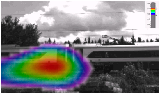
Figure 10.
Sound level distribution within a frequency range of 500–1000 Hz—straight section.
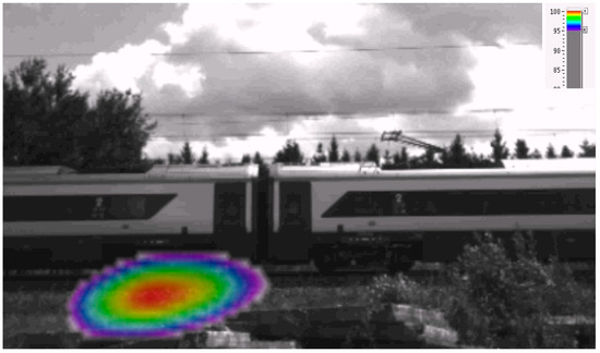
Figure 11.
Sound level distribution within a frequency range of 1000–2000 Hz—straight section.
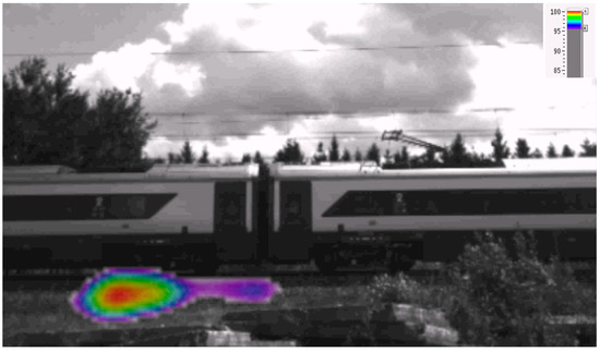
Figure 12.
Sound level distribution within a frequency range of 2000–3000 Hz—straight section.
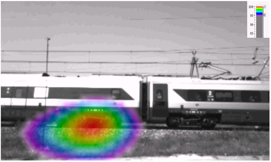
Figure 13.
Sound level distribution within a frequency range of 500–1000 Hz—curve.

Figure 14.
Sound level distribution within a frequency range of 1000–2000 Hz—curve.
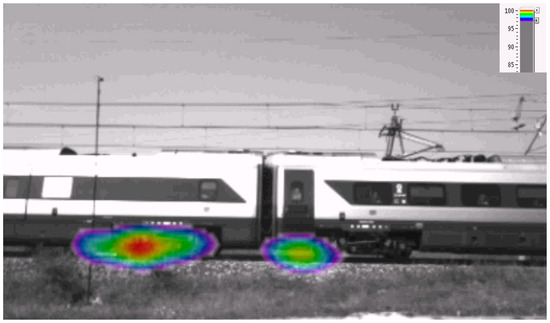
Figure 15.
Sound level distribution within a frequency range of 2000–3000 Hz—curve.
The conducted research showed that the dominant source of noise arising during the passage of high-speed railway vehicles is rolling noise originating from rail-wheel vibrations. Additionally, acoustic camera measurements of railway vehicles moving at a speed of about 200 km/h (+/−2 km/h) showed that within the studied frequency range, there were no acoustic events indicating the appearance of aerodynamic noise.
Additionally, in the case of the passage of high-speed vehicles along a curve with a radius of approximately R = 4000 m, higher sound levels in relation to the straight section could not be unambiguously stated (Table 4). In most cases, the higher energy composition (of approximately 70%), within the frequency range of 500–2000 Hz was characteristic for the curved crossings (from 2dB to 11dB); nevertheless, in approximately 30% of cases, the range of exceedances of the crossings on the straight section was higher (from 2 dB to 8 dB). In the case of sound levels, with frequencies within the range of 2000–3000 Hz, higher exceedances (55%) were recorded for passages on the straight section (difference between 1 dB and 4 dB). The obtained results of the measurements indicate that in the case of a curve with a radius of approximately R = 4000 m, it could not be unambiguously stated that the rolling noise was characterized by a higher energy composition than the straight section.
Table 4.
Comparison of the maximum sound levels in separate frequency ranges for the passage of high-speed railway vehicles on a straight section and on a curve (dB).
The comparison of average values of total acoustic wave energy density for a straight and curved track at a speed of 200 km/h is shown in Figure 16 and Figure 17.
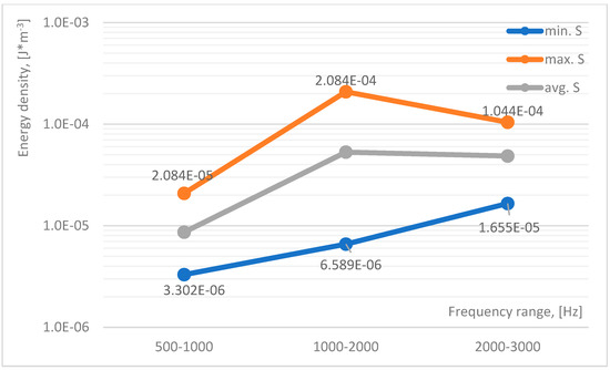
Figure 16.
The average value of the total acoustic wave energy density for a straight track, at a speed of 200 km/h.
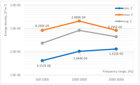
Figure 17.
The average value of the total acoustic wave energy density for the curved track at a speed of 200 km/h.
The conducted tests showed an increase in the density of acoustic energy in the frequency range 500–2000 Hz in the case of driving on a curved track and an increase in the density of acoustic energy in the frequency range of 2000–3000 Hz in the case of driving on a straight track.
Experimental research made it possible to determine which type of noise (rolling or aerodynamic) constituted the main source. The research confirmed that in the case of electric multiple traction units traveling at a speed of 200 km/h, the rolling noise, resulting from vibrations generated from wheel-rail contact, was the dominant source of noise. In the case of high-speed railway vehicles traveling along a curve with a radius of about R = 4000 m, the noise resulting from wheel-rail vibrations did not have a clear impact on increasing the maximum sound levels compared with a straight section.
Experimental tests carried out under the described conditions showed the dominance of high-frequency levels, i.e., 1.0–3.0 kHz for the straight path, and an increase in sound pressure levels, at frequencies of 0.5–1.0 kHz, for the path following the curve. In addition, the identification of dominant sound sources was successful. For the straight track, at frequencies below 1.0 kHz, the drive unit dominated. This was probably related to the operation of the gearbox or the motor itself. At frequencies above 1.0 kHz, the contact phenomena in the wheel-rail system dominated, together with the dynamic response of the infrastructure (high-frequency vibrations of the rails). For the curved track, in each case, the effects due to contact phenomena in the wheel-rail system predominated.
5. Conclusions
This paper presents research that identifies sound sources in the noise of Alstom’s high-speed train type ETR610, series ED250. The research was conducted during the passage of vehicles at a speed of 200 km/h (+/−2/3 km/h). The measuring point was located at a distance of 22 m from the track axis. Measurements were made both for the straight section and the curve, in the number of 20 measurements for each type. The identification of noise sources was carried out with the use of a 112 m acoustic camera, which made it possible to obtain results in the frequency range of 400 Hz to 24 kHz. In order to improve the properties and possibilities of locating the noise sources of high-speed trains, a beamforming method was used
The carried out measurements allowed to obtain the answer to the acoustic characteristics of the tested Alstom vehicle type ETR610, series Ed250, including the identification of the dominant noise sources. Identification of the main sources of noise from high-speed vehicles is the subject of consideration of many authors. However, an analysis of the available literature (both in Poland and internationally) has not revealed detailed measurements carried out on this type of vehicle operating at a speed of 200 km/h.
The research subject of the available work was high-speed vehicles traveling at speeds above 200 km/h, for which the main noise source was aerodynamic noise, coming mainly from the vicinity of the pantograph, windscreen, and bogies [15,16,17,18,19,20]. During the passage of a train traveling at a speed of 200 km/h, the highest sound levels are located in the bogie area, indicating that the dominant noise source is the rolling noise resulting from vibrations at the rail/wheel joint. The measured sound levels were mainly dominated by low frequencies between 500 Hz and 3000 Hz. Comparison of the results for high-speed vehicles operations on a straight section and on a curve (R = 4000 m) showed that in the frequency range between 500–2000 Hz, the curve passages had a higher sound level (70% of the crossings), while in the frequency range between 2000–3000 Hz about 55% of the straight section passages had the higher sound level.
The contribution of aerodynamic noise sources during the passage of electric multiple units traveling at about 200 km/h was not recorded. Due to some limitations of the measurements carried out, the following issues need to be considered in further work:
1. When measuring a passing vehicle, the available averaging time is very short, which may result in some uncertainty in the obtained source distribution. The introduction of additional averaging of the source distribution will enable to obtain more accurate results;
2. As the result of the identification of the main noise sources consisted mainly in taking into account the vehicle, in future the contribution of the track surface, i.e., rails, sleepers, should be taken into account.
The carried out measurements showed that the test object meets the requirements for pass-by noise specified in the TSI Noise (80 dB for vehicles traveling at 80 km/h). According to the TSI Noise guidelines, the obtained results for high-speed vehicles traveling at 200 km/h were normalized to the reference speed (80 km/h) by means of Equation (9). Based on the calculations performed, the tested high-speed vehicles obtained values of 76 dB for the straight section and 77 dB for the curve. In addition, at the distance of about 60 m from the source, the minimum requirements for protected areas in Poland were met (68 dB for the daytime in the downtown zone of cities with a population over 100,000). The research was conducted in an area where there were no acoustically protected (rural area). It should be stated that in case of occurrence of acoustically protected areas in a distance shorter than 60 m, the protection should be designed in the form of acoustic screens.
The data obtained from the experimental tests, including the results of the acoustic camera presented in the article, will allow determining the acoustic signature of Alstom vehicle type ETR610, series Ed250. Detailed identification will enable a more effective selection of measures and solutions to minimize acoustic impacts generated by such vehicles. Conducted experimental research and the database of extortions built on this basis will allow creating a universal model of dynamic excitation for the purpose of modeling impacts in the zones of influence of high-speed railway for acoustically protected areas.
Author Contributions
Conceptualization, K.P. and J.K.; methodology, J.K.; validation, J.K. and K.P.; formal analysis, J.K. and K.P.; investigation, K.P.; resources, K.P.; data curation, K.P.; writing—original draft preparation, K.P.; writing—review and editing, J.K.; visualization, K.P.; supervision, J.K.; project administration, K.P. Both authors have read and agreed to the published version of the manuscript.
Funding
Publication of this article was possible thanks to funds from the grant in the Scientific Discipline of Civil Engineering and Transport at the Warsaw University of Technology, Warsaw, Poland, 2021.
Conflicts of Interest
The authors declare no conflict of interest.
References
- Bell, J.R.; Burton, D.; Thompson, M.C.; Herbst, A.H.; Sheridan, J. Dynamics of trailing vortices in the wake of a generic high-speed train. J. Fluids Struct. 2016, 65, 238–256. [Google Scholar] [CrossRef]
- Gągorowski, A.; Korzeb, J. Road traffic noise assessment in the light of the European union and national legislation. Logistyka 2011, 6, 150–158. [Google Scholar]
- Němec, M.; Danihelová, A.; Gergeľ, T.; Gejdoš, M.; Ondrejka, V.; Danihelová, Z. Measurement and Prediction of Railway Noise Case Study from Slovakia. Int. J. Environ. Res. Public Health 2020, 17, 3616. [Google Scholar] [CrossRef]
- Wu, X.; Zhu, Y.; Xian, L.; Huang, Y. Fatigue Life Prediction for Semi-Closed Noise Barrier of High-Speed Railway under Wind Load. Sustainability 2021, 13, 2096. [Google Scholar] [CrossRef]
- Polak, K. High-Speed Rail versus environmental protection. In High-Speed Rail in Poland: Advances and Perspectives; Żurkowski, A., Ed.; CRC Press: Warsaw, Poland, 2018; pp. 421–439. [Google Scholar] [CrossRef]
- AlShorman, O.; Alkahatni, F.; Masadeh, M.; Irfan, M.; Glowacz, A.; Althobiani, F.; Kozik, J.; Glowacz, W. Sounds and acoustic emission-based early fault diagnosis of induction motor: A review study. Adv. Mech. Eng. 2021, 13, 2. [Google Scholar] [CrossRef]
- Zhao, H.; Li, Z.; Zhu, S.; Yu, Y. Valve Internal Leakage Rate Quantification Based on Factor Analysis and Wavelet-BP Neural Network Using Acoustic Emission. Appl. Sci. 2020, 10, 5544. [Google Scholar] [CrossRef]
- Ye, G.-Y.; Xu, K.-J.; Wu, W.-K. Standard deviation based acoustic emission signal analysis for detecting valve internal leakage. Sens. Actuators A Phys. 2018, 283, 340–347. [Google Scholar] [CrossRef]
- Duong, B.P.; Kim, J.; Jeong, I.; Kim, C.H.; Kim, J.-M. Acoustic Emission Burst Extraction for Multi-Level Leakage Detection in a Pipeline. Appl. Sci. 2020, 10, 1933. [Google Scholar] [CrossRef] [Green Version]
- Ahn, B.; Kim, J.; Choi, B. Artificial intelligence-based machine learning considering flow and temperature of the pipeline for leak early detection using acoustic emission. Eng. Fract. Mech. 2019, 210, 381–392. [Google Scholar] [CrossRef]
- Xargay, H.; Folino, P.; Nuñez, N.; Gómez, M.; Caggiano, A.; Martinelli, E. Acoustic emission behavior of thermally damaged self-compacting high strength fiber reinforced concrete. Constr. Build. Mater. 2018, 187, 519–530. [Google Scholar] [CrossRef]
- Xu, J.; Fu, Z.; Han, Q.; Giuseppe, L.; Alberto, C. Micro-cracking monitoring and fracture evaluation for crumb rubber concrete based on acoustic emission techniques. Struct. Health Monit. 2018, 17, 946–958. [Google Scholar] [CrossRef]
- Kitagawa, T.; Thompson, D.J. Comparison of wheel/rail noise radiation on Japanese railways using the TWINS model and microphone array measurements. J. Sound Vib. 2006, 293, 496–509. [Google Scholar] [CrossRef]
- Polak, K.; Korzeb, J. Measurements of noise from high-speed rail vehicles, Railway Problems. Pomiary hałasu pochodzącego od pojazdów kolejowych zwiększonych prędkości. Probl. Kolejnictwa 2019, 184, 33–38. (In Polish) [Google Scholar]
- Zhang, J.; Xiao, X.; Wang, D.; Yang, Y.; Fan, J. Source Contribution Analysis for Exterior Noise of a High-Speed Train: Experiments and Simulations. Shock Vib. 2018. [Google Scholar] [CrossRef] [Green Version]
- Li, M.; Zhong, S.; Deng, T.; Zhu, Z.; Sheng, X. Analysis of source contribution to pass-by noise for a moving high-speed train based on microphone array measurement Measurement. J. Int. Meas. Confed. 2021, 174, 109058. [Google Scholar] [CrossRef]
- Noh, H.M. Noise-source identification of a high-speed train by noise source level analysis. Proc. Inst. Mech. Eng. Part F J. Rail Rapid Transit. 2017, 231, 717–728. [Google Scholar] [CrossRef]
- Sheng, X.; Cheng, G.; Thompson, D.J. Modelling wheel/rail rolling noise for a highspeed train running along an infinitel long periodic slab track. J. Acoust. Soc. Am. 2020, 148, 174–190. [Google Scholar] [CrossRef]
- Zhang, J.; Xiao, X.; Sheng, X.; Li, Z. Sound Source Localisation for a High-Speed Train and Its Transfer Path to Interior Noise. Chin. J. Mech. Eng. 2019, 32, 59. [Google Scholar] [CrossRef] [Green Version]
- Wawrzyniak, A. ETR610 electric multiple units of the ED250 series for PKP Intercity, S.A. Elektrycznepociągizespołowe ETR610 serii ED250 dla PKP Intercity S.A. Tech. Transp. Szyn. 2013, 9, 20–24. (In Polish) [Google Scholar]
- Czarnecki, M.; Witold, G.; Massel, A.; Walczak, S. Introduction of High-Speed Rolling Stock into Operation on the Polish Railway Network. In High-Speed Rail in Poland: Advances and Perspectives; Żurkowski, A., Ed.; CRC Press: Warsaw, Poland, 2018; pp. 203–228. [Google Scholar] [CrossRef]
- Raczyński, J. The ED250 (Pendolino) Experiences in Poland–First Years of Exploitation. Technika Transportu Szynowego. 2018, pp. 30–32. Available online: http://yadda.icm.edu.pl/yadda/element/bwmeta1.element.baztech-9b7e36f1-647f-4ee4-aaf5-b0e7d9495dcd/c/Raczynski1TTS4en.pdf (accessed on 20 June 2021).
- Id-12 (D-29). The List of Lines, Introduced by Order No. 1/2009 of the Management Board of PKP PolskieLinieKolejowe, S.A. of 9 February 2009, as AMENDED., PKP Polskie Linie Kolejowe, 2009, In Id-12 (D-29). Wykaz linii, wprowadzony Zarządzeniem Nr 1/2009 Zarządu PKP Polskie Linie Kolejowe, S.A. z Dnia 09lutego 2009 r., z Późn.zm. (In Polish), PKP Polskie Linie Kolejowe, 2009. Available online: https://www.plk-sa.pl/files/public/user_upload/pdf/Akty_prawne_i_przepisy/Instrukcje/Wydruk/Id-12_Wykaz_linii_06.2021.pdf (accessed on 20 June 2021).
- Ordinance of the Minister of the Environment of 30 October 2014 on the Requirements for Measuring Emissions and Measuring the Smount of Water Consumed. Annex 7-Reference Methodology for Periodic Measurements of Environmental Noise from Installations or Devices, Except for Impulse Noise, Minister of the Environment 2014, In Rozporządzenie Ministra Środowiska z Dnia 30 Października 2014 r. w Sprawie Wymagań w Zakresie Prowadzenia Pomiarów Wielkości Emisji Oraz Pomiarów Ilości Pobieranej Wody. Załącznik nr 7 Metodyka Referencyjna Wykonywania Okresowych Pomiarów Hałasu w Środowisku Pochodzącego z Instalacji lub Urządzeń z Wyjątkiem Hałasu Impulsowego, Minister Środowiska, 2014. (In Polish). Available online: http://isap.sejm.gov.pl/isap.nsf/DocDetails.xsp?id=WDU20190002286 (accessed on 20 June 2021).
- Kołaski, W.; Arnold, A. Decrease in noise level as a function of distance from source. Spadek poziomu hałasu w funkcji odległości od źródła, OchronaŚrodowiska. J. Pol. Sanit. Eng. Assoc. 1982, 3, 26–28. Available online: http://www.os.not.pl/docs/czasopismo/1982/Kolaski_3-1982.pdf (accessed on 20 June 2021). (In Polish).
- Puzyna, C. Noise reduction in industry. General principles. In Zwalczaniehałasu w Przemyśle; Zasadyogólne WNT: Warszawa, Poland, 1974. (In Polish) [Google Scholar]
- Technical Specification of an Acoustic Camera Bionic M-112. Available online: http://www.wibroakustyka.com.pl/dokumenty/datasheet_acoustic_camera_bionic_m_112.pdf (accessed on 14 May 2021).
- Cigada, A.; Lurati, M.; Ripamonti, F.; Vanali, M. Moving microphone arrays to reduce spatial aliasing in the beamforming technique: Theoretical background and numerical investigation. J. Acoust. Soc. Am. 2008, 124, 3648–3658. [Google Scholar] [CrossRef] [PubMed]
- Dwyer-Joyce, R.S.; Yao, C.; Lewis, R.A. Comparison of three methods for the measurement of wheel rail contact. In Proceedings of the STLE/ASME International Joint Tribology Conference, Miami, FL, USA, 20–22 October 2008; pp. 541–543. [Google Scholar] [CrossRef]
- Graf, H.R.; Czolbe, C. Pass-by noise source identification for railroad cars using array measurements. In Proceedings of the International Congress on Acoustics, Aachen, Germany, 9–13 September 2019; pp. 1574–1581. [Google Scholar]
- Motylewski, J.; Pawłowski, P.; Rak, M.; Zieliński, T.G. Identification of sources of vibroacoustic activity in machines by beam shaping (beamforming). In Identyfikacja Źróde Łaktywności Wibroakustycznej Maszyn Metodą Kształtowania Wiązki Sygnału (Beamforming), XXXVII Polish SYMPOSIUM on Machine Diagnostics; PWN: Warszawa, Poland, 2010; pp. 1–8. (In Polish) [Google Scholar]
- Zhang, J.; Squicciarini, G.; Thompson, D.J. Implications of the directivity of railway noise sources for their quantification using conventional beamforming. J. Sound Vib. 2019, 459, 114841. [Google Scholar] [CrossRef]
- Noh, H.-M.; Choi, S.; Kim, S.-W.; Koh, H.-I. Aerodynamic noise characteristics of a specific position of a passing high-speed train by the beam power spectrum. In Proceedings of the 41st International Congress and Exposition on Noise Control Engineering, New York, NY, USA, 19–22 August 2012; Volume 8, pp. 6309–6316. [Google Scholar]
- Polak, F.; Sikorski, W.; Siodła, K. Prototype measurement system for locating sources of acoustic emission-microphone matrix (in Polish Prototypowy układ pomiarowy do lokalizacji źródeł emisji akustycznej–matryca mikrofonów), Poznan University of Technology Academic Journals. Electr. Eng. 2015, 84, 207–214. [Google Scholar]
- Gade, S.; Ginn, B.; Gomes, J.; Hald, J. Recent advances in rail vehicle moving source beamforming, Sound & Vibration. In Proceedings of the INTER-NOISE and NOISE-CON Congress and Conference Proceedings, Innsbrug, Austria, 15–18 September 2013; pp. 8–14. [Google Scholar]
- Le Courtois, F.; Thomas, J.-H.; Poisson, F.; Pascal, J.-C. Genetic optimisation of a plane array geometry for beamforming. Application to source localisation in a high speed train. J. Sound Vib. 2016, 371, 78–93. [Google Scholar] [CrossRef]
- Meng, F.; Wefers, F.; Vorlaender, M. Acquisition of exterior multiple sound sources for train auralization based on beamforming. In Proceedings of the Euronoise 2015, 10th European Conference on Noise Control, Maastricht, The Netherlands, 31 May–3 June 2015; pp. 1703–1708. [Google Scholar]
- Chiariotti, P.; Martarell, M.; Castellini, P. Acoustic Beamforming for Noise Source Localization—Reviews, Methodology and Applications. Mech. Syst. Signal Process 2019, 120, 422–448. [Google Scholar] [CrossRef]
- He, B.; Xiao, X.-B.; Zhou, Q.; Li, Z.-H.; Jin, X.-S. Investigation into external noise of a high-speed train at different speeds. J. Zhejiang Univ. Sci. A 2014, 15, 1019–1033. [Google Scholar] [CrossRef] [Green Version]
- Qi, L.; Zeng, Z.; Zhang, Y.; Sun, L.; Rui, X.; Li, X.; Wang, L.; Liu, T.; Yue, G. Research on Leakage Location of Spacecraft in Orbit Based on Frequency Weighting Matrix Beamforming Algorithm by Lamb Waves. Appl. Sci. 2020, 10, 1201. [Google Scholar] [CrossRef] [Green Version]
- Korzeb, J. Prediction of selected dynamic impacts in the transport infrastructure influence zone. In Redykcja Wybranych Oddziaływań Dynamicznych w Strefie Wpływu Infrastruktury Transportowej; OWPW: Warszawa, Poland, 2013; p. 202. ISBN 978-83-7814-111-2. (In Polish) [Google Scholar]
- Nader, M. Vibrations and noise in transport: Selected issues. In Drgania i Hałas w Transporcie: Wybrane Zagadnienia; Oficyna Wydawnicza Politechniki Warszawskiej: Warszawa, Poland, 2016. (In Polish) [Google Scholar]
- Rosssing, T. (Ed.) Springer Handbook of Acoustics; Springer: New York, NY, USA, 2014. [Google Scholar] [CrossRef]
- Ozimek, E. Sound and its perception. Physical and psychoacoustic aspects. In Dźwięk i jego percepcja. Aspekty fizyczne i Psychoakustyczne; PWN: Warszawa, Poland, 2018. (In Polish) [Google Scholar]
- Beranek, L.; Mellow, T. Acoustics: Sound Fields, Transducers and Vibration; Academic Press: Cambridge, MA, USA, 2019. [Google Scholar]
- Commission Regulation (EU). No 1304/2014 of 26 November 2014 on the Technical Specification for Interoperability Relating to the Subsystem ‘Rolling Stock—Noise’ Amending. Decision 2008/232/EC and Repealing Decision 2011/229/EU. 2011. Available online: https://eur-lex.europa.eu/legal-content/EN/TXT/?uri=CELEX:32014R1304 (accessed on 20 June 2021).
- Regulation of the Minister of Environment of 14 June 2007 on Permissible Noise Levels in the Environment; Minister of Environment 2007. In Rozporządzenie Ministra Środowiska z dnia 14 Czerwca 2007 r. w Sprawie Dopuszczalnych Poziomów Hałasu w Środowiska (Tekst Jednolity Dz.U. 2014 poz. 112); Minister Środowiska: Warsaw, Poland, 2007. Available online: http://isap.sejm.gov.pl/isap.nsf/DocDetails.xsp?id=WDU20140000112 (accessed on 20 June 2021). (In Polish)
Publisher’s Note: MDPI stays neutral with regard to jurisdictional claims in published maps and institutional affiliations. |
© 2021 by the authors. Licensee MDPI, Basel, Switzerland. This article is an open access article distributed under the terms and conditions of the Creative Commons Attribution (CC BY) license (https://creativecommons.org/licenses/by/4.0/).