Field-Ready Implementation of Linear Economic Model Predictive Control for Microgrid Dispatch in Small and Medium Enterprises

Abstract

The increasing share of distributed renewable energy resources (DER) in the grid entails a paradigm shift in energy system operation demanding more flexibility on the prosumer side. In this work we show an implementation of linear economic model predictive control (MPC) for flexible microgrid dispatch based on time-variable electricity prices. We focus on small and medium enterprises (SME) where information and communications technology (ICT) is available on an industrial level. Our implementation uses field devices and is evaluated in a hardware-in-the-loop (HiL) test bench to achieve high technological maturity. We use available forecasting techniques for power demand and renewable energy generation and evaluate their influence on energy system operation compared to optimal operation under perfect knowledge of the future and compared to a status-quo operation strategy without control. The evaluation scenarios are based on an extensive electricity price analysis to increase representativeness of the simulation results and are based on the use of historic real-world measurements in an existing production facility. Due to real-world restrictions (imperfect forecast knowledge, implementation on field hardware, power fluctuations), between 72.2% and 85.5% of the economic optimum (rather than 100%) is reached. Together with reduced operation cost, the economic MPC implementation on field-typical industrial ICT leads to an increased share of renewable energy demand.

1. Introduction

With the shift from predominantly fossil-fuel-based electricity generation towards an energy system primarily based on renewable energy sources, new operational challenges for the electrical grid arise. A high penetration of renewable energy sources in the grid entails a paradigm shift in the utility grid operation, because electricity demand needs to be adapted to a certain degree for renewable energy generation. One of various methods for renewable energy supply and electricity demand to meet is demand side management (DSM) [1]. Flexibilization on the demand side should be incentivized by energy scarcity and excess pricing signals, and should be automated through information and communications technology [2,3]. European electricity providers with more than 200,000 customers are required to offer dynamic price contracts by the directive of the European parliament and of the council of 5 June 2019 on common rules for the internal market for electricity [4]. Rather small electricity retailers already offer time-variable energy tariffs on the German market [5,6,7].

To date, the energy system operation strategy of households and small and medium enterprises (SMEs) usually is to maximize the own consumption of on-site distributed renewable energy (DER). This is due to privileged own-consumption tariffs and static energy supply tariffs and does not comply with the goal of flexibilization. Literature abounds with energy management strategies in the residential sector, whereas we focus particularly on SMEs since they have high DSM potential. This potential results from incorporating plannable electric vehicle (EV) fleets, large roof-mounted photovoltaic (PV) energy systems on production facilities, dual-use of battery storage for energy management and uninterruptible power supply, and existing ICT for the automated implementation of DSM measures. ICT in SMEs often contains programmable logic controllers (PLCs) of IEC 61131 standard with application-specific IOs and fieldbuses [8], which we will use in our work.

A promising approach for the incorporation of DSM in microgrids is economic model predictive control (MPC). This optimization-based technique has been shown to be beneficial for microgrid operation involving battery storage, EVs, and renewable generation [9,10,11,12,13]. It allows to take the predictability of the controlled system into account and enables economically driven operation strategies depending on time-variable prices. However, the implementations described in the literature are often simulation-only and are implemented on desktop or workstation hard- and software [13,14,15]. Moreover, the forecast data used to predict renewable energy sources often implies perfect knowledge of the future. Other work focuses on peak shaving and disregards time-variable electricity tariffs [16]. Hardware implementations of MPC were shown for energy systems but often use Matlab or similar desktop/workstation software for tertiary control (optimization, MPC) and underlying interfacing with Labview or SCADA devices for primary/secondary control of energy system components [16,17,18,19]. The authors of [20] report on a field-hardware-only implementation of a tracking MPC for a distillation column. To this end, they ported MPC algorithms to the IEC 61131 programming language on a PLC. More recently, in [21] an MPC was implemented in IEC 61131 code by code generation from MATLAB, which results in code that can be hard to maintain or modify.

The use of MPC in embedded systems is still limited by implementability and dependability issues (dependability is used as a collective term for the time-related quality characteristics of a system and includes concepts such as availability, reliability, recoverability, maintainability, maintenance support performance, durability, safety, and security) [22,23]. Requirements, that we fulfil in our field-ready implementation of economic MPC for energy systems, are the incorporation of typical SME energy system components, implementation on field-suitable hardware only, prediction but imperfect knowledge of future PV power and aggregated power consumption, problem formulation such that commissioning is limited to parametrization (complexity reduction), and increase of operation reliability, safety, and security by hardware-in-the-loop (HiL) testing. The article addresses the research gap from simulation papers (mostly in the residential sector or single specific plants) and hardware implementation based on workstations towards on-site and stand-alone implementations on field-hardware (industrial ICT) with a reasonable trade-off between commissioning effort and optimisation results, keeping the rather low economic savings potential with today’s typical price structure in mind.

This paper extends the preliminary study presented in [24] to include electric mobility, simulation of more representative scenarios with longer duration, and comparison of MPC results under uncertainty of forecasts with the theoretical optimal solution under perfect forecasting knowledge.

2. Materials and Methods

This section describes our linear model of a microgrid, the MPC formulation, and implementation on field-typical hardware. The underlying predictions of pricing, PV and load power are outlined, too. Furthermore, an experimental performance evaluation of the field-ready implementation by HiL testing is described. The conditions and scenarios of these experiments are also described in this chapter.

2.1. System Modelling and Implementation Specifics

The basic idea of economic MPC is to repeatedly solve a constrained optimization problem with receding horizon and an objective function that represents an economic objective [25]. Therefore, it is necessary to establish a mathematical model of the controlled system, or plant. This section describes the system model, the objective function, and implementation specifics.

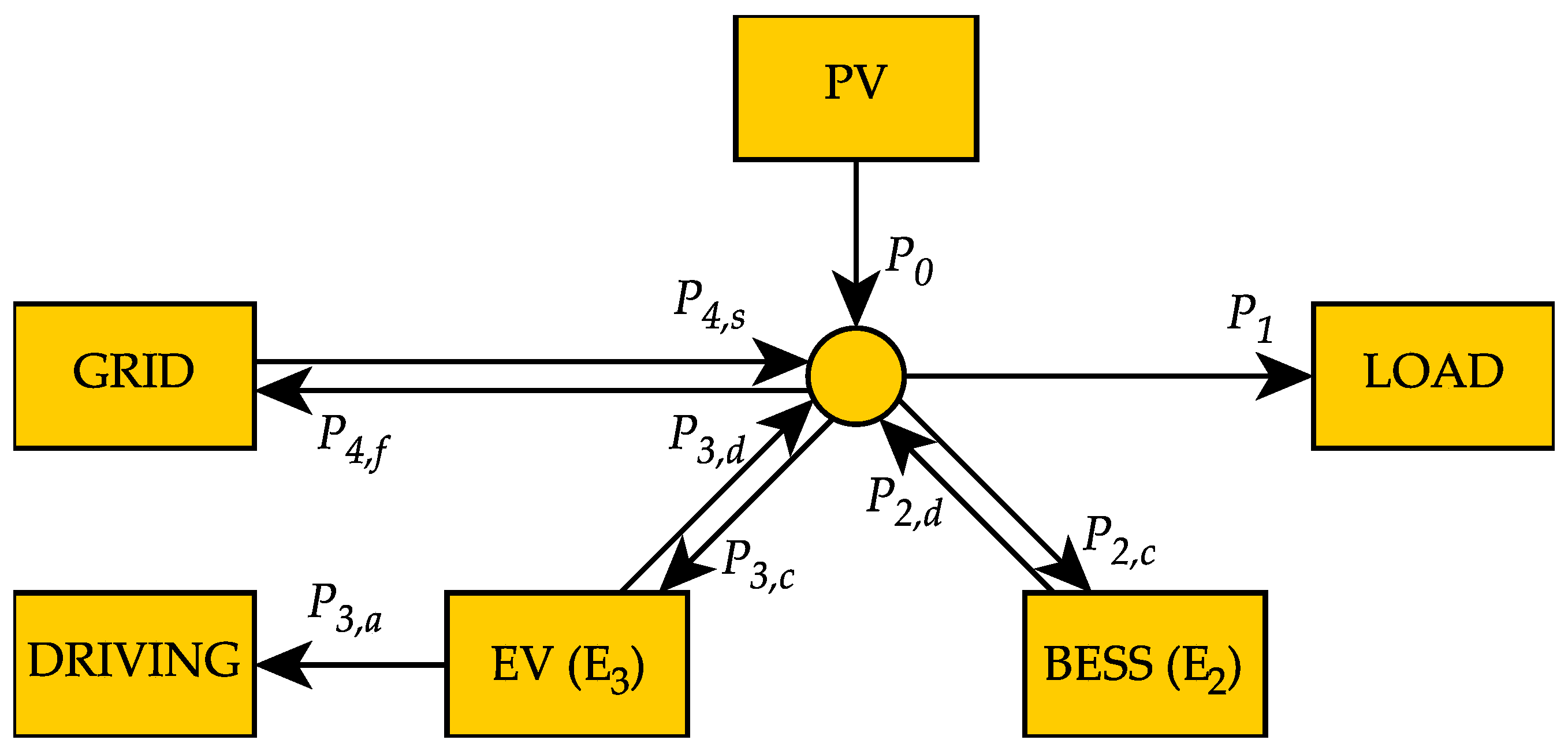
2.1.1. System Modelling

The system model that is used in an MPC controller must provide information about the future state as a function of the current state and of current and future inputs. This model can be formulated in various forms such as differential equations, state-space representation, transfer function representation, or discrete difference equations but also artifical neural network (ANN) models [26]. In this work, we use an explicit discrete state space representation. The goal is to develop this MPC implementation for use in SME microgrids. Therefore, the system architecture and the constraints were chosen with an existing production facility in mind, used as a representative example.

The components of the energy system model and their associated active powers are depicted in Figure 1. The system consists of a PV power plant (power output $P_0$), a single immutable load ($P_1$) which represents the aggregated power demand of the production facility and must be met at all time, a battery storage (charging power $P_{2,c}$, discharging power $P_{2,d}$, energy content $E_2$) for dual use (uninterruptible power supply and DSM), an EV (charging power $P_{3,c}$, discharging power $P_{3,d}$, energy content $E_3$), and a connection to the central power grid. The grid can serve as source ($P_{4,s}$) or as a sink for for feed-in of surplus renewable energy ($P_{4,f}$). The absent discharging of the vehicle battery by driving is modelled with a discharge power $P_{3,a}$. Transmission losses due to cabling etc., are neglected as they could not be determined with reasonable effort in practical commissioning situations.

The energy conservation in the local microgrid and in the two storage components and the power prediction for the PV plant and the load leads to the discrete linear model equations

$$P_0^k+P_{2,d}^k+P_{3,d}^k+P_{4,s}^k-(P_1^k+P_{2,c}^k+P_{3,c}^k+P_{4,f}^k)=0,$$

(1)

$$E_2^{k+1}-E_2^k=\Delta t\times ({\eta }_{2,c}\times P_{2,c}^k-1/{\eta }_{2,d}\times P_{2,d}^k),$$

(2)

$$E_3^{k+1}-E_3^k=\Delta t\times ({\eta }_{3,c}\times P_{3,c}^k-1/{\eta }_{3,d}\times P_{3,d}^k-P_{3,a}^k),$$

(3)

$$P_0^k=P_{\mathrm{pv},\mathrm{f}}^k,\mathrm{and}$$

(4)

$$P_1^k=P_{\mathrm{load},\mathrm{f}}^k.$$

(5)

Here,

$$P_i^k=P_i(t=t_k)\mathrm{with}{t}_k=k\Delta t$$

(6)

denotes the active power exchanges of component i at timestep k, and

$$E_i^k=E_i(t=t_k)$$

(7)

are the energy contents of the battery storage $(i=2)$ and the electric vehicle battery $(i=3)$ at timestep k. The time interval $\Delta t$ is the time difference between discretization steps (the sampling interval). ${\eta }_{i,c}$ and ${\eta }_{i,d}$ are the charging and discharging round-trip efficiencies of battery storage and electric vehicle, which are assumed to be constant. While in reality the efficiency depends on C-rate, aging, $SOC$, etc. [27], the assumption of constant efficiencies does not contribute larger errors than the many unknown disturbances and uncertainties associated with systems the parameters of which cannot be identified completely for economic reasons. The fact that the assumption preserves the linearity of the problem, justifies its use in these circumstances. $P_{\mathrm{pv},\mathrm{f}}^k$ and $P_{\mathrm{load},\mathrm{f}}^k$ are the respective PV and load power forecasts at timestep k (see Section 2.2).

German grid regulations allow the feed-in from battery electric storage systems (BESS) or EV to the utility grid if these components can only be charged by on-site renewable generation, but not from the grid. Because we want to exploit time-variable energy prices by storing cheaper energy in the BESS, this means that the feed-in from BESS or EV to the local microgrid must be less than the total power consumption to avoid feed-in into the utility grid:

$$P_{2,d}^k+P_{3,d}^k-P_1^k-P_{2,c}^k-P_{3,c}^k\le 0.$$

(8)

Additional constraints hold because of limitations in the rated power of components and cabling,

$$0\le P_i^k\le P_{i,\max },$$

(9)

as well as limitations in the energy content of the BESS and EV,

$$SO{C}_{i,\min }\times C_i\le E_i^k\le SO{C}_{i,\max }\times C_i$$

(10)

for all k, with minimum and maximum permitted state of charge (SOC) and the component capacities $C_i$. An SOC operating window which is a subset of 0% to 100% is advisable to increase the lifespan of the batteries, or to guarantee uninterruptible power supply for a certain amount of time in case of grid faults. It may also be useful to limit or stop the vehicle’s feed into the local grid to increase its battery life:

$$P_{3,d}^k\le P_{3,d,\max }^k.$$

(11)

The end user may want to guarantee certain minimum SOCs for their EVs at selected points in time, depending on their fleet planning. A target SOC for the EV at timestep k can be formulated as

$$SO{C}_{\min }\times C_3\le E_3^k.$$

(12)

We minimize the economic cost function

$$J=\sum _{k=0}^{N-1}l(c_i^k,P_i^k)=\Delta t\times \sum _{k=0}^{N-1}(-c_{\mathrm{feed}-\mathrm{in}}\times P_{4,f}^k+c_{\mathrm{supply}}^k\times P_{4,s}^k)$$

(13)

over a finite time horizon subject to the equality constraints (1)–(5), inequality con-straint (8) and lower and upper bounds (9)–(12). The economic costs are calculated with a fixed feed-in tariff $c_{\mathrm{feed}-\mathrm{in}}$ and time-dependent electricity supply prices $c_{\mathrm{supply}}^k$, the step size $\Delta t$ over the number of time steps N resulting in a prediction horizon of $t_{\mathrm{p}}=N\times \Delta t$. To ensure reasonably foresighted fleet planning, a prediction horizon of $t_{\mathrm{p}}=$48 h was chosen. The discretization time step $\Delta t$ is 15 min, which is a common billing period in energy economics. This results in $N=192$ timesteps.

In this formulation, the charging and discharging powers of the storage units are independent. In theory, this allows the simultaneous charging and discharging of storage units, which is physically unreasonable. However, this condition could only occur, if the power exchange between microgrid and utility grid were constrained and PV generation were larger than the power demand, such that excess energy would have to be consumed. Otherwise, simultaneous charge and discharge leads to energy losses and therefore costs, that are avoided in the optimization by feeding surplus PV energy into the grid. Power exchange between the microgrid and the utility grid is not constrained, as the grid connection in the modelled production facility sustains simultaneous maximum power demand of EV, BESS, and load. Subsequently, simultaneous charging and discharging does not occur.

A similar problem exists for the power exchange of the microgrid with the main grid. Simultaneous demand and feed-in are physically not reasonable, but possible in our formulation if the price for electricity supply were less than the feed-in tariff. For the tariff we evaluated, this is not the case. Nonetheless, lower retail prices might occur in the future, even though feed-in tariffs for DERs are expected to further decrease as well. If this case only occurs rarely, a simple mitigation is to treat such prices as equal to the feed-in tariff. This of course discards optimality and no longer reflects actual economic costs, but avoids a mixed integer formulation. With increasing frequency of lower retail prices, this would have to be reconsidered. Simultaneous charging and discharging can be avoided by hiding nonlinearity with mixed logical dynamical system modeling [9,28]. However, this results in a MILP, which we avoid.

With the state vector

$$x:=(E_0,E_1,P_0,\dots ,P_5),$$

(14)

where

$$P_i:=(P_i^0,\dots ,P_i^{N-1})\mathrm{and}$$

(15)

$$E_i:=(E_i^0,\dots ,E_i^N),$$

(16)

the equations, which have to be solved at every iteration, can be written in general form of a linear programming (LP) problem, also called linear optimization problem, with linear constraints and linear cost function:

$$\begin{array}{cc}\hfill \underset{x}{\min }& \phantom{=}{c}^{T}x\hfill \end{array}$$

(17)

$$\begin{array}{cc}\hfill \mathrm{s}.\mathrm{t}.& \phantom{=}{A}_{eq}x=b_{eq},\hfill \end{array}$$

(18)

$$\begin{array}{cc}\hfill & \phantom{=}{A}_{ub}x\le b_{ub},\mathrm{and}\hfill \end{array}$$

(19)

$$\begin{array}{cc}\hfill & \phantom{=}l\le x\le u\hfill \end{array}$$

(20)

with a specific cost vector c containing the cost of energy supply and revenue from feed-in, lower and upper bounds l and u, equality and upper bound inequality constraint matrices $A_{eq}$ and $A_{ub}$, and equality and inequality constraint vectors $b_{eq}$ and $b_{ub}$. These quantities have the dimensions

$$\begin{array}{cc}\hfill P_i& \in {\mathbb{R}}^N,\hfill \end{array}$$

(21)

$$\begin{array}{cc}\hfill E_i& \in {\mathbb{R}}^{N+1},\hfill \end{array}$$

(22)

$$\begin{array}{cc}\hfill c,x,l,u& \in {\mathbb{R}}^{11N+2},\hfill \end{array}$$

(23)

$$\begin{array}{cc}\hfill b_{eq}& \in {\mathbb{R}}^{5N+2},\hfill \end{array}$$

(24)

$$\begin{array}{cc}\hfill A_{eq}& \in {\mathbb{R}}^{(5N+2)\times (11N+2)},\hfill \end{array}$$

(25)

$$\begin{array}{cc}\hfill b_{ub}& \in {\mathbb{R}}^{N+2},\mathrm{and}\hfill \end{array}$$

(26)

$$\begin{array}{cc}\hfill A_{ub}& \in {\mathbb{R}}^{(N+2)\times (11N+2)}.\hfill \end{array}$$

(27)

In the context of MPC, the constrained optimization problem (17)–(20) is solved repeatedly, proceeding as follows:

• Sample system state: SOC measurements, prediction of PV power and aggregated power demand
• Solve constrained optimization problem using the recently sampled state and the predictions from step 1 for the prediction horizon $t_p$;
• Apply first elements of the optimal control sequence of the decision variables $P_{2,c}$, $P_{2,d}$, $P_{3_c}$, and $P_{3,d}$ to the energy system for a specific control horizon $t_c$;
• Repeat after defined interval with a receding prediction horizon

The control horizon $t_c$ is chosen to be equal to the step size $\Delta t$, i.e., only the first element of the optimal control sequence is applied. The forecast of PV power and power demand is assumed to be more representative for the following 15 min than the recently measured value, which is why the prediced PV and load powers are used as system state variables.

The decision to use an LP formulation as described above is also motivated by the requirement of independence from high performance but expensive commercial solvers and by the requirement of embedded (low-performance) hardware. Furthermore, questions about reachability of global optimality, computational complexity, determination of runtime, and lower bounds for the objective function can be answered deterministically for linear formulation. This ultimately benefits reliability.

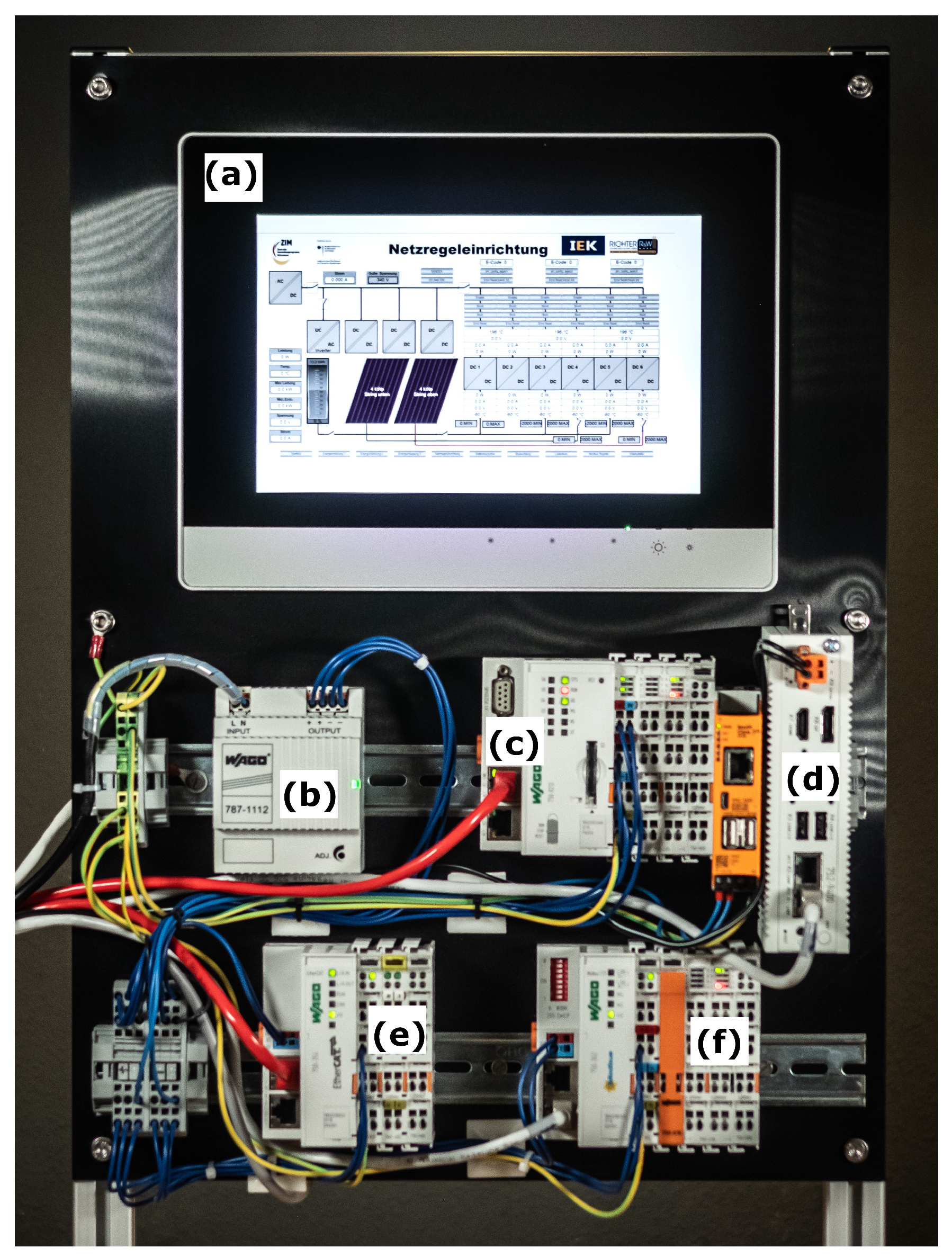
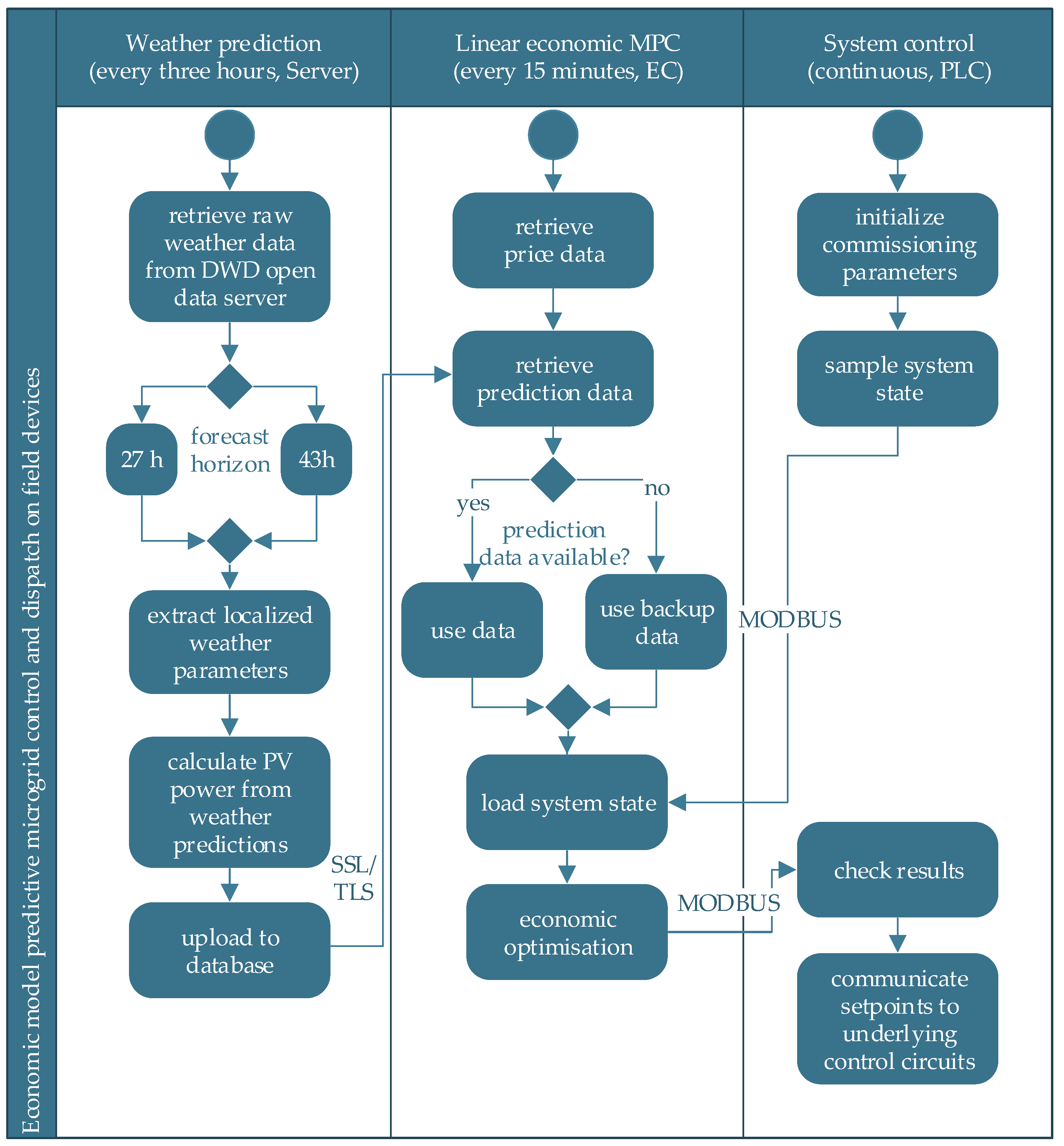
2.1.2. Hardware and Software Implementation

Our MPC has been implemented on industrial hardware mounted on DIN rails, which is typically used enclosure systems (see Figure 2). The hardware, on which the optimization runs, is a field device of the type “Wago Edge Computer, 752-940x” based on an Intel Atom E3845 quad-core processor with $1.91$ GHz running Linux. A PLC of the type “Wago PFC 200, 750-8212” is used for measurements in the energy system (system sampling) and the communication of set-points to underlying controllers like the battery controller or the communication with the EV.

In this way, measurement and component control on the one side and operational planning on the other side are clearly separated. This separation is important for

• commissioning: The parametrization of the MPC system parameters (storage capacities, bounds, efficiencies, ...) is done on the PLC and is available to the edge computer (EC) via Modbus, such that the commissioning engineer only requires IEC 61131 knowledge;
• reliability: Independent devices for supervisory control and underlying component control, such that fallback mechanisms in case of MPC failure can be implemented in the PLC;
• maintainability: separation of devices and modularization simplifies maintenance and further development;
• IT security: Independent devices provide different rights management, different interfacing (local and web), and media discontinuity.

The implementation on field-devices led to specific software requirements. Optimization is computationally expensive, such that the limited computing power of typical ICT components was taken into account. Moreover, desktop/workstation software like MATLAB was avoided and independent (stand-alone) solver implementations were used. Additionally, specific requirements for licensing were considered. Open-source solvers, licensed with strong copyleft, may not be usable if commercialization of the MPC solution is intended. On the other hand, the price of commercial solvers might exceed potential savings. We decided to use the linprog solver, distributed with Python’s Scipy package, which is licensed under a permissive BSD license. This solver is a Python implementation of the interior point method. The optimization is triggered every 15 min by the operation system’s scheduler resulting in high triggering precision of less than 7 $\mathsf{\mu }$s. Figure 3 shows an activity diagram of the software implementation.

While simulation studies allow the user to examine exceptional cases such as failing solver convergence, unusually many iterations, or other particularities in more detail, there is no such easy way of monitoring in real-time field implementations. This requires the field implementation to be much more reliable. This is why the PLC carries out a feasibility check. Optimization results are not applied to the energy system unchecked. Only if the optimization algorithm exits successfully, results are applied to the system by the PLC. Success of optimization is communicated to the PLC via Modbus. Otherwise, the system is set to a fail-safe mode (e.g., deactivation of the storage or EV charging on maximum power regardless of pricing). Fail-safe operation can be defined by the commissioning engineer in IEC 61131 code. Furthermore, the PLC is responsible for redundancy in constraint satisfaction. Optimization results are compared again with the bounds, set by the commissioning engineer. In case of bounds violation (e.g., due to MPC implementation faults), the PLC uses fail-safe operation mode. In addition, the PLC is responsible for the inequality constraint satisfaction of (8). Direct application of the optimization results with a 15-min resolution could lead to constraint violation (e.g., battery feed-in to the grid when power demand is lower than predicted). The PLC avoids this by continuously monitoring the inequality constraint and restricting the setpoints in case of violation. Moreover, the commissioner can implement special behaviour for scenarios outside of planned operation (e.g., power outages of the grid). Further reliability measures can be found in [22], where fault handling is categorized in fault prevention, fault tolerance, fault detection, fault removal and fault prediction. Fault removal and prediction are not covered in our work.

Unsuspecting end users might configure lower EV SOC bounds that are infeasible due to insufficient charging time or power. For this reason, the feasibility of SOC bounds is checked before optimization and infeasible bounds are changed to the maximum feasible lower bound. In this way, the vehicle is charged to the highest SOC that can be achieved in the remaining time. For a linear problem under investigation, which is convex, choosing the constraints in a reasonable and pre-checked way avoids infeasibility, which is why slack variables as proposed in [22] are not applied, because this would increase the problem size.

2.2. Predictions of Electricity Prices, Power Demand and PV Power

A crucial advantage of MPC over error tracking methods like PID controllers is its ability to take knowledge about the future into account. This applies both to system dynamics and to external disturbances. PV power and aggregated consumer power as well as electricity prices can be considered external disturbances. These variables can be predicted to a certain degree. Prediction methods and accuracy measures are described in the following subsections, the evaluation of predictor accuracy is shown in Section 3.

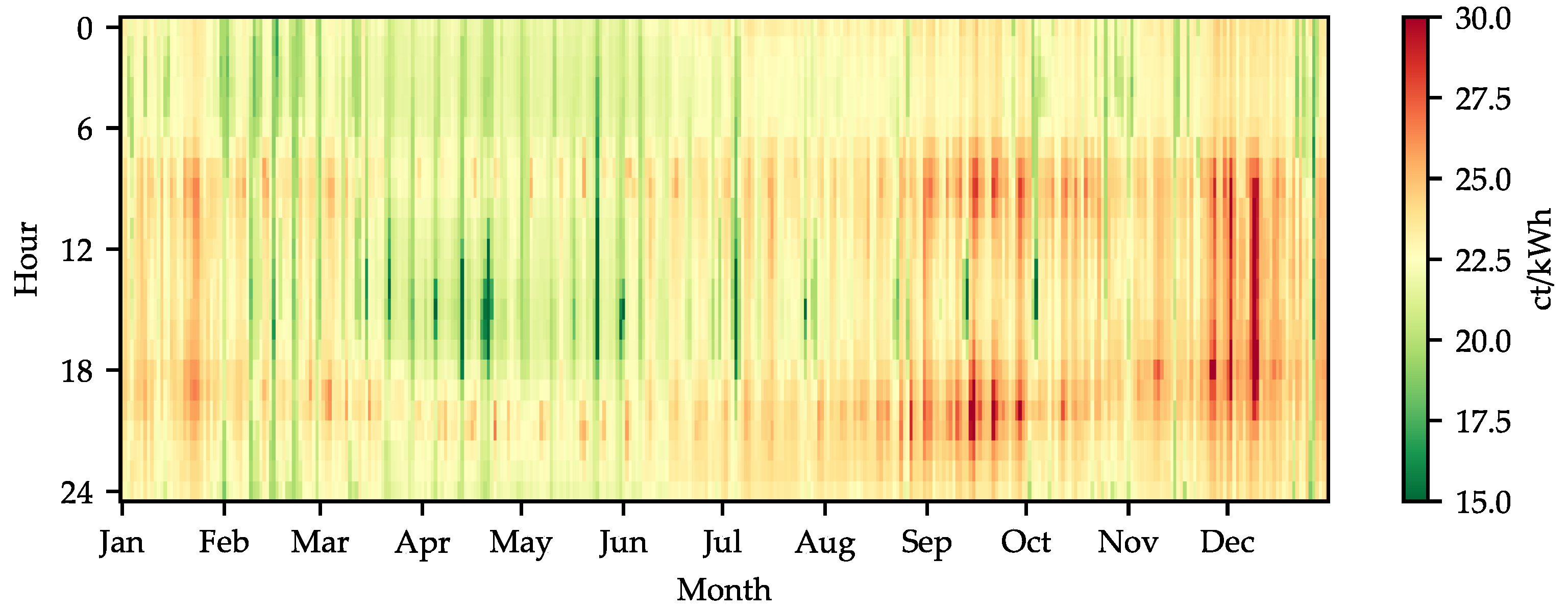
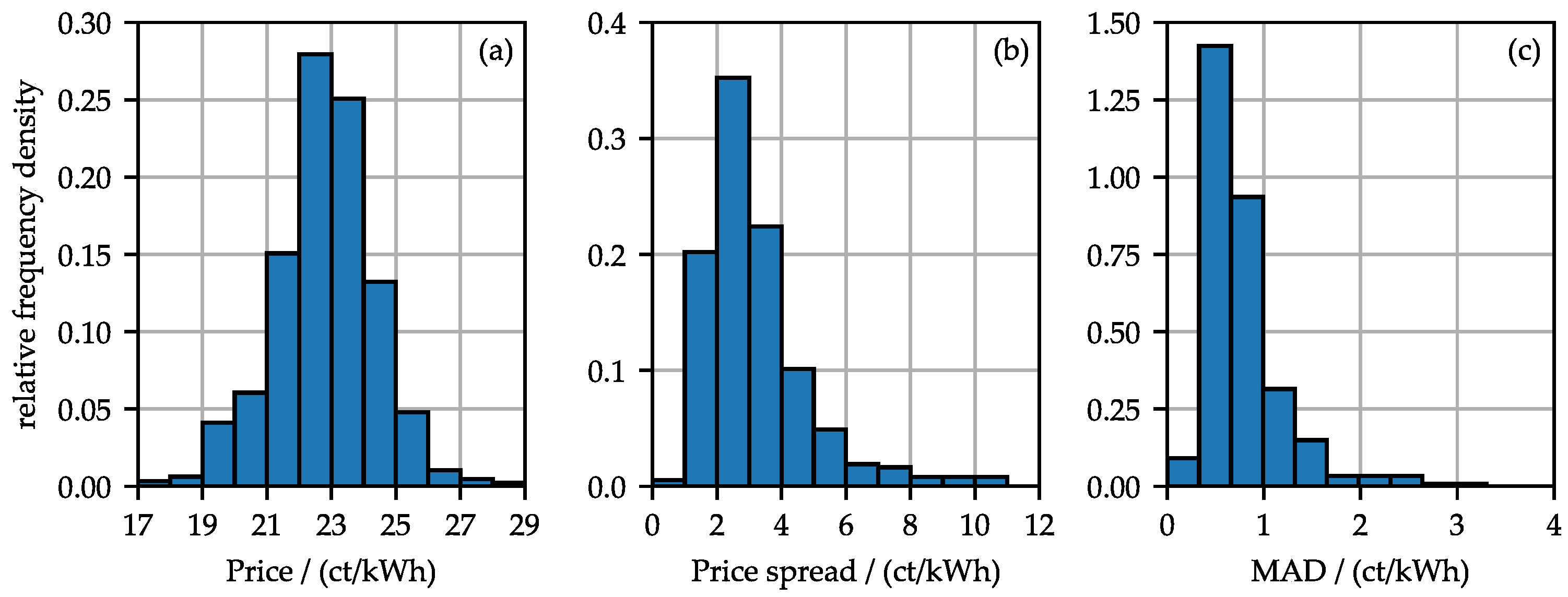
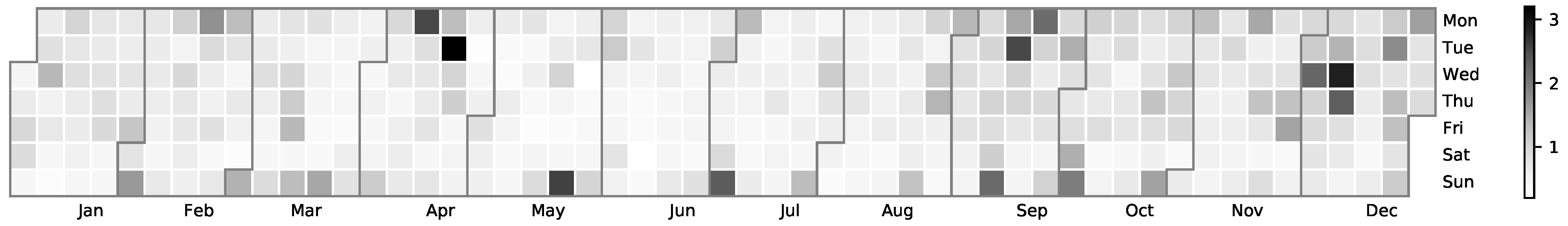
2.2.1. Price Forecasts and Price Analysis

The EU directive on common rules for the internal market for electricity [4] stipulates that beginning in 2021 electricity suppliers with more than 200,000 customers must offer electricity tariffs representing real-time pricing signals based on spot market prices. Some rather small electricity providers are already offering such time-variable tariffs on the German retail market [5,6,7]. In this implementation, the price API of [5] is used, which is representative for dynamic tariffs that pass on electricity exchange prices. This electricity tariff is composed of a fixed basic charge per kWh and hourly variable charges, which depend on the day-ahead market clearing prices at the European power exchange. Retail prices for the following day are made available by the supplier daily at 2 p.m., which is when market clearing at the European power exchange takes place. This means that secure price information is available for a forecast horizon between $10.25$ h (at 1.45 p.m. until midnight of the same day) and 34 h (at 2 p.m. until midnight of the next day). Since the optimization horizon is 48 h, price information for the remaining hours is necessary. For these remaining hours, mean prices from historic price data of 52 weeks $\mathcal{W}=\{w\in \mathbb{N}|1\le d\le 52\}$ in 2020 were used. These were calculated for every type of day $\mathcal{D}=\{d\in \mathbb{N}|1\le d\le 7\}$ and hour $\mathcal{H}=\{h\in \mathbb{N}|1\le d\le 24\}$ resulting in 168 hourly prices

$$c_{\mathrm{supply},\mathrm{mean}}(h,d)=\frac{1}{52}\sum _{w=1}^{52}{c}_{\mathrm{supply}}(h,d,w).$$

(28)

Moreover, the daily price spread and mean absolute deviation from daily mean prices in 2020 were calculated. This analysis gives further insight into electricity pricing and provides information on the suitability of pricing in terms of economic DSM potential. In the literature, simulation scenarios often are referred to as typical days, but their informative value is limited due to the non-transparent selection of these days. The price analysis supported the selection of scenarios serving to evaluate the MPC implementation. The intraday price spread

$$c_{\mathrm{spread}}(d,w)=\underset{h\in \mathcal{H}}{max}\left(c_{\mathrm{supply}}(h,d,w)\right)-\underset{h\in \mathcal{H}}{min}\left(c_{\mathrm{supply}}(h,d,w)\right))$$

(29)

is the difference between daily maximum price and daily minimum price for electricity. The daily price spread alone is not a good indicator for DSM potential of the respective day, because the duration of price fluctuations is just as important for the exploitation of dynamic pricing as the spread. Hence, the mean absolute deviation (MAD)

$$MAD(d,w)=\frac{1}{24}\times \sum _{h=1}^{24}|c_{\mathrm{supply}}(h,d,w)-\overline{c}(d,w)|$$

(30)

of hourly prices from the daily mean price

$${\overline{c}}_{\mathrm{supply}}(d,w)=\frac{1}{24}\times \sum _{h=1}^{24}\left(c_{\mathrm{supply}}(h,d,w)\right)$$

(31)

is a better measure of DSM potential because it takes the duration of price fluctuations into account. The evaluation of relative frequency density of prices, MAD, and intraday price spreads is shown in Section 3. The feed-in tariff for PV power feed-in is not time-variable and defined in German feed-in legislation EEG. In this work, the tariff for plants commissioned in August 2020 is used, which amounts to $8.9$ ct/kWh.

2.2.2. Photovoltaic Power Predictions

The PV power generation at the production facility is predicted by an online implementation using external numerical weather prediction (NWP) data from the German weather service (DWD) and physical PV models as described in previous work [29]. In the first step, prediction data of relevant weather parameters (irradiance, temperature, wind speed, etc.) from the COSMO-D2 NWP model of the DWD is downloaded from the open data server of the DWD [30] to a local server. These weather predictions are provided with a 15-min to 1-h resolution, depending on the parameter, and for the whole model area of Germany in GRIB2 format. These raw data are then processed using the software package ecCode [31] of the European Centre for Medium-Range Weather Forecasts (ECMWF) to extract localized parameters for the location of the PV power plant. The extracted localized weather parameters are then used for PV power calculations using the pvlib-python library, which provides Python implementations of physical PV modelling [32]. The PVWatts physical model of National Renewable Energy Laboratory (NREL) was used for our predictions [33]. The DC power of PV module arrays is calculated from plane-of-array irradiance $E_{\mathrm{poa}}$, the nameplate power $P_{\mathrm{dc}0}$ at standard test conditions, the temperature coefficient ${\gamma }_{\mathrm{pdc}}$, and the cell and reference temperatures $T_{\mathrm{cell}}$ and $T_{\mathrm{ref}}$ by

$$P_{dc}=\frac{E_{\mathrm{poa}}}{1000}{P}_{\mathrm{dc}0}(1+{\gamma }_{\mathrm{pdc}}(T_{\mathrm{cell}}-T_{\mathrm{ref}})).$$

(32)

Furthermore, inverter and cabling losses are considered. The DWD runs the COSMO-D2 model every three hours starting at 12 a.m. coordinated universal time (UTC) with a forecast horizon of 27 h each, except for the model run at 3 a.m. UTC, which has a forecast horizon of 45 h. The PV power forecast implementation is automated to recalculate the PV output power with each weather prediction release by the DWD.

The PV power predictions depend on the provisioning of data from the DWD and on internet access. For reasons of reliability, the penultimate and third-last forecasts are always used in addition to the most recent forecast. This bridges up to nine hours of data provisioning downtime. Furthermore, the 3 a.m. forecast is always used due to its longer prediction horizon. Priority is always given to the most recent prediction data. As the power prediction forecast of 27 to 45 h does not cover the 48-h optimization horizon, the power output beyond NWP predictions is modelled as half-sine wave during daytime at time of day $t_{\mathrm{tod}}$

$$p_{\mathrm{pv}}\left(t_{\mathrm{tod}}\right)=p_{\mathrm{pv},\max }\times sin\left(\frac{\pi (t_{\mathrm{tod}}-t_{\mathrm{sr}})}{t_{\mathrm{dl}}}\right).$$

(33)

Here, $p_{\mathrm{pv},\max }$ denotes the maximum intra-day power, $t_{\mathrm{sr}}$—the time of sunrise, $t_{\mathrm{dl}}$ —the daytime duration, and $p_{\mathrm{pv},\max }$—a peak power depending on the season (winter, summer, transition) and based on historic PV plant measurement data. This prediction method is used as fallback method in case of failing data provisioning and on the far end of the prediction horizon beyond NWP data. The influence of imperfect predictions on the far end of the forecast horizon is low, as shown in [24], such that this method is suitable as addition to the NWP based prediction.

Data-driven models were not considered here for practical reasons. For widespread application in SMEs it is necessary to obtain solid prediction data from day one without the need of model training and protracted data acquisition. This can be achieved by physical modeling. Moreover, the authors of [34] have found that data-driven models (trained on five years worth of data) show similar performance as their physical model using COSMO-D2 data of DWD.

2.2.3. Power Demand Predictions

The aggregated power demand of the production facility is modelled as a single and immutable power consumer. From the analysis of historic electricity-demand data, it became clear that the electricity demand of the investigated production facility quite stably follows a pattern that mainly depends on the working hours of the company. The aggregated demand was therefore modelled by averaging of one year of historic data, similar to the price forecasts. The prediction distinguishes between weekdays (Monday to Thursday), Friday, Saturday, and Sunday, and uses a 15-min resolution such that each demand profile consists of 96 values. While this is a simple approach, it is sufficient for this field implementation. It could possibly be improved by more sophisticated methods, however, the influence on the control performance depends on the load variability of the SME and a reasonable trade-off between simplicity of commissioning and control performance gains is required.

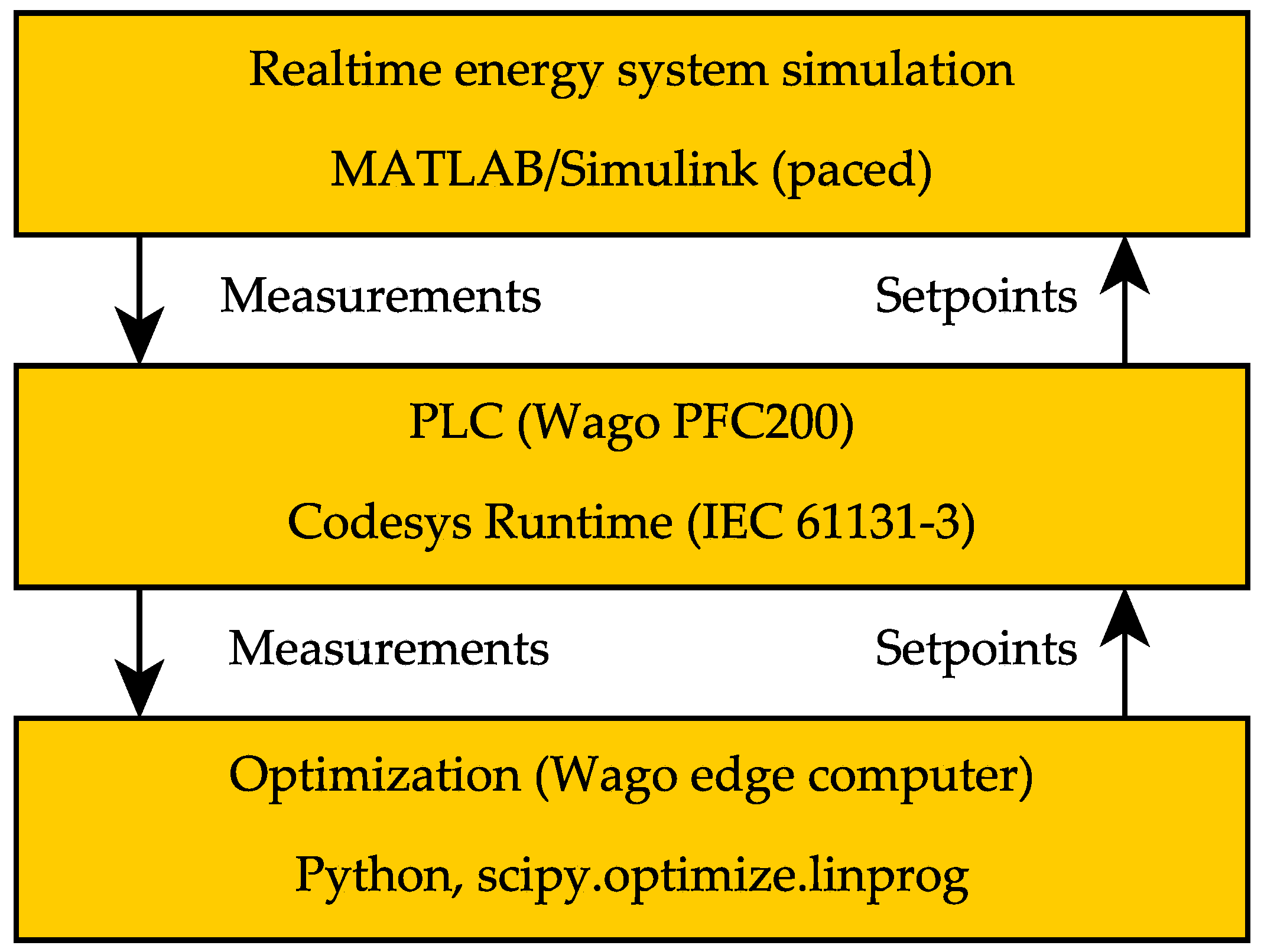
2.3. HiL Simulations

The field-ready MPC implementation described in Section 2.1 was tested in a HiL testbench, based on previous work described in [35]. The following subsections provide details about the system architecture of the testbench, the simulation conditions, and evaluated scenarios.

2.3.1. HiL System Architecture

For safety and security reasons, the controller implementation described in Section 2.1 cannot simply be characterized and tested in the real-world production environment of the facility (the “field”). However, testing of the implementation should cover as many aspects as possible that occur in the field. For this reason, the energy system of the production facility was modelled as a digital twin in MATLAB/Simulink with real-time execution on a workstation computer. The simulation model matches the controller model, except for the battery model, for which a generic model from the Matlab/Simulink Simscape library was used. The library model is more comprehensive than the integrator in the controller model. This results in a model mismatch that will also exist when controlling the energy system in the production facilty. The MPC hardware implementation and the simulation model communicate via the same field interfaces that are used in the production facility, viz., MODBUS/TCP and CAN. Interfaces and protocols are realized as in the field components in the production facility, such that the controller implementation under test in this virtual environment is an identical twin of the field controller in the production. This makes for a high technology readiness level prior to the actual field implementation. The system structure is shown in Figure 4.

2.3.2. Simulation Acceleration and Synchronization

In order to be representative for the real operating behaviour of the field-ready hardware implementation, the simulation in the HiL experiment must run in real-time. To evaluate the MPC implementation over a long period of time (e.g., days or weeks), the HiL experiment would require an equally long simulation duration. If one wants to treat different scenarios, as we did, one has to accelerate the simulation times. This is limited by the computing power of the HiL simulation computer and the field hardware (PLC, EC). The HiL simulation computer and the PLC allow acceleration without influencing the simulation results as long as the CPU of both components is below full load and as long as their processes are worked off in specified cycle times. Another factor limiting the acceleration is the invariant computation power of the EC, which solves the constrained optimization. In non-accelerated mode, optimizing a 48-h interval with 15-min resolution requires about 6 s of CPU time, i.e., the optimization solution is applied to the energy system 6 s after the start of each quarter hour. Due to the acceleration of the surrounding HiL simulation, this time interval scales linearly with the acceleration factor. An acceleration factor of 2 for the HiL-simulation means that the optimizer’s solution is applied to the energy system virtually 12 s after the start of each quarter hour. We limited the acceleration factor to 5, which results in a delay of 24 virtual seconds, in order to limit the distorting influence of the delayed arrival of the optimization results at the energy system. Yet, this allowed us to investigate significantly more scenarios per time.

Another issue we considered is synchronization and time drift. The devices should of course be synchronized such that the HiL simulation and the optimization device operate on the same simulation time. Nevertheless, the optimization device should remain close to the real field behaviour. External triggering of the MPC is therefore unwanted. Initial synchronization was achieved by setting the date and time of the EC from Matlab via SSH at the start of simulation. Both computers show usual clock drift, resulting from their internal clock mechanism, as the EC cannot be synchronized to NTP servers when historic scenarios are simulated. Therefore the clock drift of the EC compared to the simulation computer was determined in advance and added proportionally to the simulation acceleration factor. Subsequently, simulation and optimization devices showed clock drifts of less than one second for a simulation scenario of two weeks and an initial synchronization offset of zero seconds.

2.3.3. Scenarios for HiL Simulation

The HiL experiments were conducted with two representative scenarios. These scenarios were constructed from historic measurements of PV power and power demand at the production facility, which was then operated without any control strategy or BESS. The scenarios were selected based on the results of the price analysis. In addition, only prediction data of the corresponding days that were available at that time were used for the simulations (no ex-post knowledge). The scenarios and the reason for their selection are presented below. The HiL scenario simulation data has a resolution of 10 s. This is necessary to cover fluctuations in the PV and load powers.

In both scenarios, the BESS has a capacity of $C_2=13.8 \mathrm{kWh}$, SOC limits of $SO{C}_{2,\min }=10\%$ and $SO{C}_{2,\max }=90\%$, a maximum charge power of $P_{2,\mathrm{c}}\le 5 \mathrm{kW}$, a maximum discharge power of $P_{2,\mathrm{d}}\le 3 \mathrm{kW}$, and a charging/discharging efficiency of ${\eta }_2=96\%$. The EV has a capacity of $C_3=77 \mathrm{kWh}$, a charging efficiency of ${\eta }_3=96\%$, a charging-power limit of $P_{3,\mathrm{c}}\le 11$ kW, and no vehicle-to-grid function ($P_{3,\mathrm{d}}=0$). The PV power plant has a nominal power of $8.44$ kW. The EV is a commuting vehicle the presence pattern of which was taken from historic usage data. It is planned to arrive at 6 a.m. local time with an SOC of 10% and to leave at 5 p.m. with an SOC of 90% for seven days a week. There is no mismatch between planned and actual EV behavior.

Scenario 1

The first scenario is based on the two-week interval from 3–16 August 2020. During these two weeks, the MAD from daily average prices was exceptionally low (see Figure 8). The minimum MAD was $0.35$ ct on 15 August, the maximum MAD was $0.75$ ct on 6 August. As a result, the economic leverage from flexible prices is comparatively low in this scenario. With mostly sunny weather, PV energy generation was high, which then resulted in surplus feed-in of 85 kWh without control intervention. The economic leverage from avoiding surplus feed-in is comparatively high in this scenario, since a feed-in tariff of $8.9$ ct/kWh is applied and the mean electricity price over the two weeks is $23.17$ ct/kWh. The difference can be exploited by avoiding feed-in via load shifting, thus increasing self-consumption when PV generation is high.

Scenario 2

The second scenario is based on the two-week interval from 14–27 September 2020. At the beginning of both weeks, the MAD from daily mean prices was exceptionally high ( $2.53$ ct on 15 September, $2.15$ ct on 21 September, $1.53$ ct on 14 September, see also Figure 8). Nine of fourteen days have a higher price MAD, than the maximum price MAD in Scenario 1 ( $0.75$ ct). The cost leverage from flexible prices is comparably high. Moreover, PV power generation is quite high resulting in surplus feed-in of 92 kWh without control intervention. The mean electricity supply price for the two weeks was $24.32$ ct/kWh.

2.3.4. Scenario Evaluation

The HiL simulation results with field-ready MPC operation strategy are compared to two other operation strategies, acting as benchmark strategies:

(a)

Status-quo operation strategy

(b)

Ex-post optimal operation

With (a) there is no dedicated control strategy, i.e., surplus feed-in occurs when PV excess energy is generated, no BESS is used, and the EV is charged on arrival until a threshold SOC of 90% is reached. This benchmark is used to determine improvements compared to the status-quo. With (b) the scenario is optimized ex-post under perfect predictor knowledge (knowledge of 15-min mean values of power demand and PV generation). This benchmark is used to determined the upper bound of achievable improvements. The scenario is actually optimized for 16 days and evaluated at the end of day 14 to avoid emptying of the BESS towards the end of the horizon, which occurs due to the economic optimization. The determined optimal EV and BESS charging curves are used to determine the residual load at the grid connection point, where total cost of feed-in and supply for operation strategy (b) is calculated.

A comparison with other implementations described in the literature is only of very limited value, since scenarios, components and system dynamics and are generally rather specific and results are not directly transferable. Therefore, a comparison with ex-post optimal operation is preferable and is chosen in this work. Moreover, to the best of the author’s knowledge, there are no peer-reviewed publications on real-time, on-site implementations on field typical hardware (industrial ICT) without cloud dependendy in the non-residential sector as of today.

In addition, the energy supplied by the grid is analyzed with regard to the hourly share of renewable or conventional energy on the basis of market data from the German Federal Network Agency [36]. In this way, the amount of renewable and conventional energy supplied from the utility grid was determined in each scenario and operation strategy.

3. Results

In this section, we present results in four categories: (1) Price analysis of the chosen tariff [5], which is representative for German energy exchange prices; (2) evaluation of the load and PV forecasts; (3) verification of the controller model; and (4) evaluation of the performace of our implementation by a comparison with the two benchmark operation strategies (a) and (b).

3.1. Electricity Price Analysis

A heatmap representation of hourly electricity prices reveals an accumulation of high prices in the morning and evening hours, and lower prices during night-time and early afternoon (Figure 5). This is plausible as grid power demand peaks in the morning and evening hours. Moreover, the share of PV power is highest around noon. This suggests that demand flexibilization (which intends to exploit flexible price) has a typical daily pattern. This synergizes with daily EV usage patterns and the relatively small storage capacities of EVs and BESSs. Seasonal price fluctuations are not exploitable with the small capacity storage of (small) stationary BESSs and of EVs.

Table 1. Yearly average of: Intraday mean price depending, intraday price spread, and intraday MAD depending on the type of day, calculated from historic price data of the year 2020 in ct/kWh.

	Mon	Tue	Wed	Thu	Fri	Sat	Sun
Mean price	23.94	23.10	23.25	23.23	23.07	22.29	21.54
Mean price spread	3.14	2.70	2.26	2.39	1.96	1.53	2.69
MAD	0.71	0.60	0.58	0.56	0.49	0.32	0.61

shows the yearly average of daily mean price, intraday price spread, and intraday MAD from daily mean price depending on the type of day in 2020. The price spread but also MAD can be observed to peak on Mondays and decrease throughout the week rising again on Sunday. The daily mean price is highest on Monday, relatively stable during the week, and lowest on the weekend.

In Figure 6 the relative frequency distribution of hourly electricity prices $c_{\mathrm{supply}}(h,d,w)$, intraday price spreads $c_{\mathrm{spread}}(h,d,w)$, and mean absolute deviations $MAD(d,w)$ from corresponding daily mean prices $\overline{c}(d,w)$ are shown for the year 2020. The hourly prices appear to be normally distributed throughout the year. The intraday price spread shows positive skewness. This means that high price spreads occur rather rarely and the mass of intraday price spreads occur in the lower range. The same applies for the MAD from daily mean prices. This keeps the potential of economic return from DSM through load shifting rather low. Or, to put it differently, higher intraday spreads and MADs are desirable in Germany in the future if one wants to effectively influence consumer behaviour by time-variable electricity pricing.

Figure 7 shows all hourly electricity prices in the year 2020 and the corresponding share of renewable energy in the German utility grid at each hour. The market data of renewable energy share is available at the SMARD data platform of the German Federal Network Agency [36]. The correlation coefficient is $r=-0.73$. This high negative correlation between prices and renewable share is explained by the fact that stock-market electricity prices are determined by the merit-order principle. Renewable energy displaces fossil energy on the market due to the difference in their marginal costs. A high share of renewable energy shifts the merit-order supply curve meeting demand at lower marginal prices. Conversely, a flexibilization on the demand side based on economic optimization would effectively reduce the ${\mathrm{CO}}_2$ footprint of electricity demand by shifting the demand towards hours with higher renewable energy share.

Figure 8 shows a yearly heatmap of the mean absolute deviation of electricity prices from the corresponding daily mean price for electricity. This information was used to find time periods that represent typical situations in the electricity market for the evaluation of our MPC solution. Economic leverage lies in load shifting towards times when electricity prices are more favorable as well as load shifting towards times when PV power generation exceeds power demand. The price spread and MAD of electricity prices is significantly lower than the price spread between grid supply and feed-in tariff, which makes the second lever economically more influential. All prices in this evaluation are net prices.

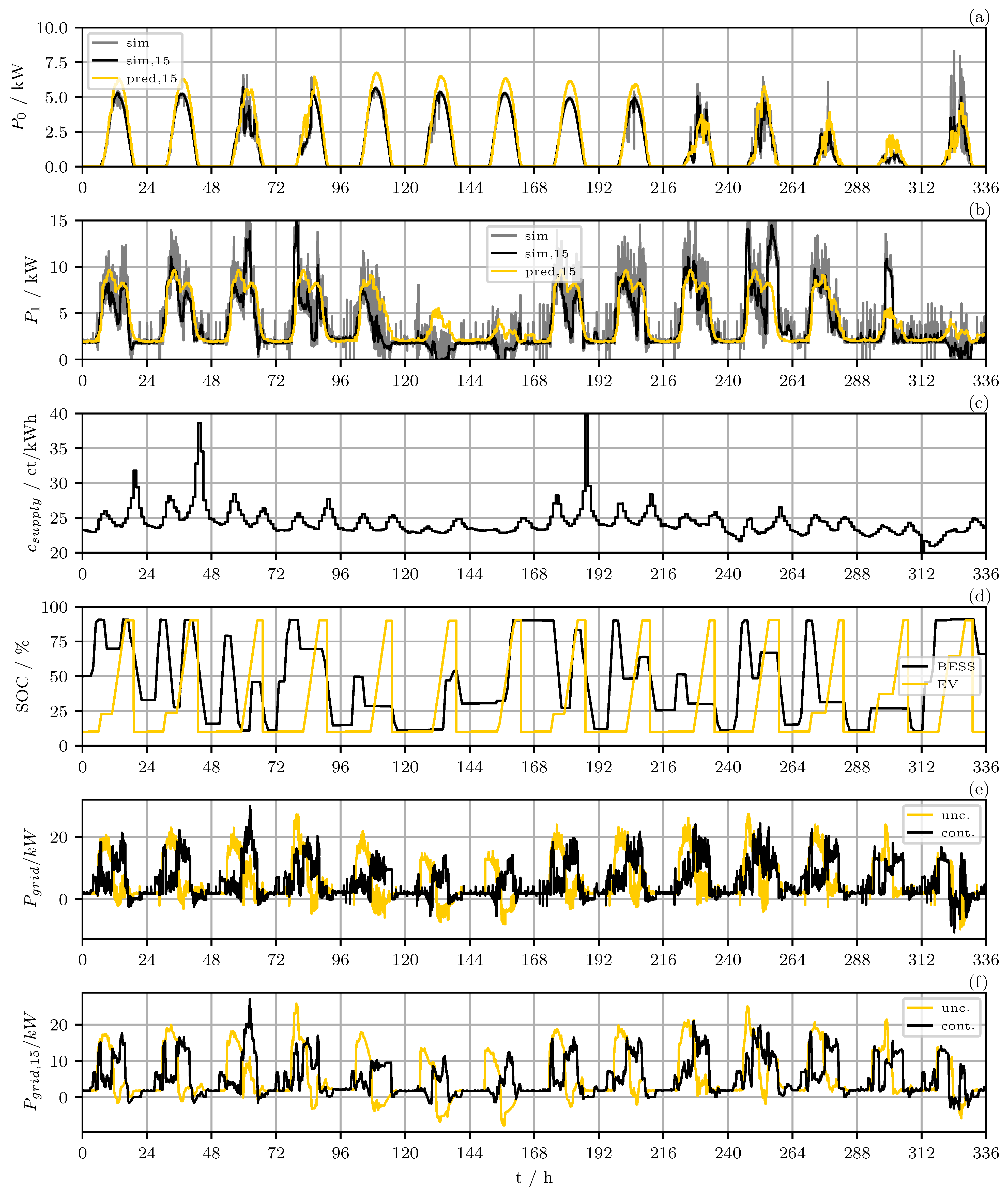
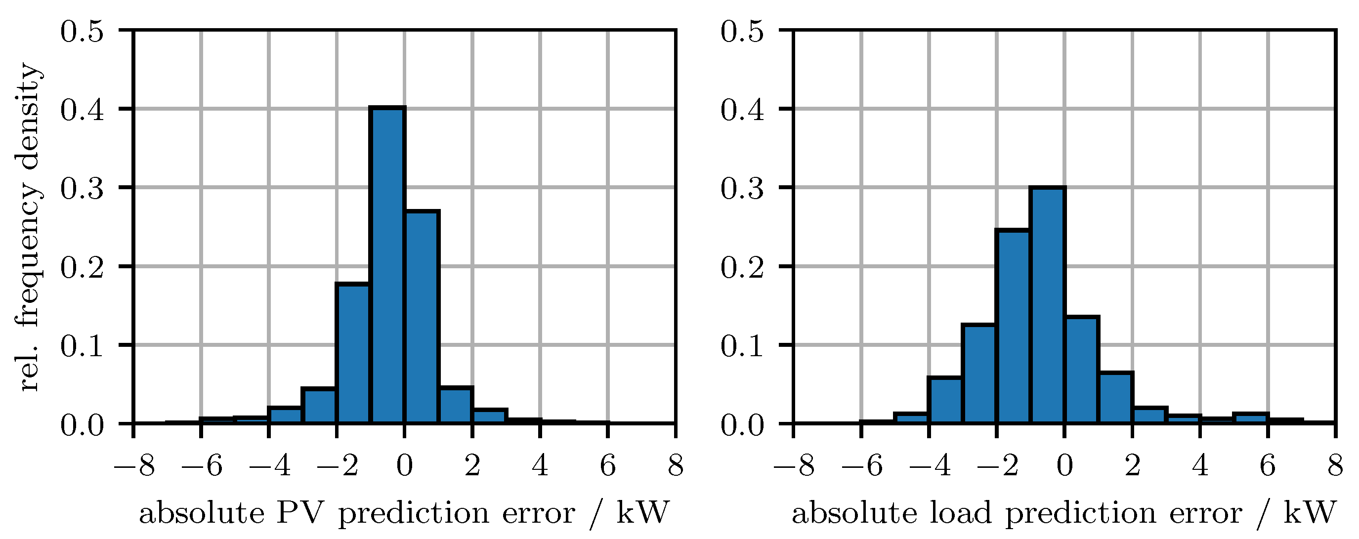
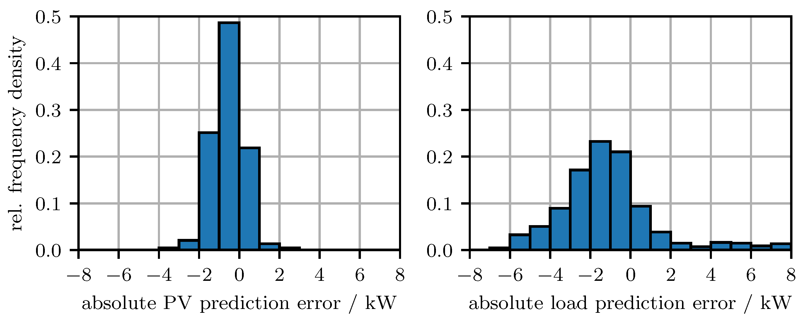
3.2. PV and Load Power Predictions

During the operation of the power system, the PV power predictions are updated every three hours, which is when the NWP model is issued by the DWD. To compare the forecast in the two scenarios with the actually measured PV power, a two week best-case forecast was created by stitching the first 3 h of every issue together. These forecasts are believed to be the most reliable, which is why they are also used as state sample for the MPC instead of measurements. The relative frequency density of the absolute prediction error $P_{\mathrm{err}}=P_{\mathrm{sim}}-P_{\mathrm{pred}}$ is shown in Figure 9 for Scenario 1 and in Figure 10 for Scenario 2. In each case, 15-min mean values are compared. Positive errors describe underestimation, negative errors mean overestimation of the power. Only power generation during daytime was considered in this analysis. The power forecasts of both components show substantial errors. All forecasts show a tendency towards overestimation.

3.3. Controller Model Verification

The correct implementation of the controller model was verified by implementing the same linear system model not in Scipy but using the PuLP modeling language [37]. The open-source solver CBC [38] was used to find optimal solutions under various representative scenarios. As expected, the optimization results of the SciPy implementation and the PuLP/CBC implementation are the same, since LPs are convex and global optimality is achieved whenever the solver converges.

3.4. Performance Evaluation of the Hardware Implementation

Table 2. Operational cost comparison of simulated scenarios.

	Scenario 1			Scenario 2
Cost	Total	Supply	Feed-in	Total	Supply	Feed-in
Status quo	401.03 €	408.59 €	−7.56 €	440.75 €	448.85 €	−8.10 €
Ex-post optimal	385.70 €	386.54 €	−0.84 €	415.49 €	416.35 €	−0.86 €
MPC, HiL	387.92 €	388.93 €	−1.01 €	422.52 €	424.13 €	−1.61 €

shows the operational cost of both simulated scenarios. In Scenario 1, a cost reduction of 13.11 € was achieved. This amounts to 85.5% of the possible cost reduction in this scenario of 15.33 €. In Scenario 2, operational costs could be reduced by 18.23 €, or 72.2% of the possible cost reduction in this scenario of 25.26 €. The cost reduction consists of avoided surplus feed-in and shifted energy supply from the grid while prices are low. These numbers show, that economic MPC on field devices with state of the art forecasting achieves a large part of the theoretically possible savings.

Controlling the energy system with our MPC implementation also changes the share of renewable and fossil-fuel-based energy supplied by the grid, because lower prices correlate with higher shares of renewable energy in the utility grid (see Figure 7). In Scenario 1, renewable energy share from the utility grid is increased to 43.8% from 40.7% while at the same time reducing the total amount of energy from the utility grid by 4.0% due to increased own consumption. In Scenario 2, renewable energy share from the utility grid is increased to 44.1% from 41.3% while at the same time reducing the total amount of energy from the utility grid by 2.7%.

Table 3. Energy from utility grid: Renewable energy (ren.), renewable energy share from grid, conventional energy (conv.), conventional share from grid, total energy from grid and reduction of utility-grid energy due to increased DER own consumption in ex-post optimal case and MPC controlled case (HiL-experiment) for both scenarios.

	Ren. Energy	ren. Share	conv. Energy	conv. Share	Total	Reduction
Status quo S1	712.5 kWh	40.7%	1037.2 kWh	59.3%	1749.7 kWh
Ex-post opt. S1	733.9 kWh	43.8%	0941.4 kWh	56.2%	1675.3 kWh	4.2%
MPC, HiL S1	736.1 kWh	43.8%	0943.7 kWh	56.2%	1679.8 kWh	4.0%
Status quo S2	750.0 kWh	41.3%	1068.0 kWh	58.7%	1818.0 kWh
Ex-post opt. S2	768.9 kWh	44.2%	0970.7 kWh	55.8%	1739.6 kWh	4.3%
MPC, HiL S2	780.2 kWh	44.1%	0989.5 kWh	55.9%	1769.7 kWh	2.7%

shows amounts and shares of renewable energy and conventional energy supplied by the utility grid.

A comprehensive graphical presentation of the simulation results in both scenarios can be found in Appendices Appendix A.1 and Appendix A.2. Subplot (d) shows the SOC of BESS and EV. EV charging is distributed throughout the day by maximizing PV self-consumption and making use of low energy prices until the EV minimum threshold $SO{C}_{min}=90\%$ is reached. The BESS is typically discharged in the morning hours when prices and load demand are high, and typically charged by excess PV energy and from the grid when prices are low. Subplots (e) and (f) show the residual loads at the grid connection point in the uncontrolled and controlled scenarios. The proposed control modifies the uncontrolled scenario patterns by avoiding most of the surplus feed-in of PV power and and typically shifting power demand towards afternoon, when energy prices are typically lower. This control behaviour makes immediate sense and reproduces what fuzzy rules described in language form would call for.

4. Discussion

Today, there can be not doubt that machine learning and big-data methods allow one to optimize large-scale energy systems. This viewpoint is that of utilities, which must ensure security of supply for many consumers, and also the viewpoint expressed in many published works. In such applications, the effort for modeling and operating a control system is almost irrelevant, because these efforts can be allocated to many consumers and because statistical influences can be modeled very well due to the law of large numbers.

In this work, we have tried to take a different viewpoint, viz., that of small industrial prosumers who attempt to optimize their use of electric energy and to minimize cost. In such applications it is usually not possible to fully model the system, identify all system parameters, collect data over extended periods of time, compromise production for commissioning, parameterization, and possibly even troubleshooting of new control equipment, use hardware or software that is expensive or otherwise unsuitable for field use, etc., The presented implementation takes these restrictions into account. With it, flexible control equipment for electric power systems can be put into operation with manageable effort.

Again, there exist methods which provide better prediction results in specific and individual cases (e.g., no overestimation of PV power or better prediction of load requirements). Data-driven predictor methods spring to the mind, but they require resources (hardware, software, time for data acquisition and learning) which, under practical demands, are often unreasonable. Moreover, prediction methods can be improved incrementally if the current trade-off between commissioning effort and potential for economic improvement in microgrid operation is considered unfavorable as price structures change in the future. For now, achieving as little as 50% of the theoretical optimum at a normalized overall cost of 1 beats achieving 90% of the theoretical optimum at a total cost of 10.

5. Conclusions

Demand side management through economic MPC on field typical ICT using available forecasting techniques is beneficial regarding cost reduction for the facility operator, regarding reduction of fossil fuel based electricity demand and regarding increase of own consumption. An optimal operation may not be reached with imperfect forecasts, but we achieved a large part of theoretically possible savings (up to 85%). A high technology readiness level was achieved by HiL-testing the ICT in a digital twin of the energy system. We added practical aspects to existing research on MPC for power systems (to date mainly consisting of simulation-only studies) and show that field implementations are possible and useful.

However, to further the flexible use of regenerative energy, there is a need for a higher economic incentive. As our results have clearly shown, the current German pricing structure is a serious obstacle to the goal of flexible regenerative energy use. This goal can best be realized by increasing the variable share of energy prices compared to the fixed share of energy prices (fees, taxes). We also expect price spreads to increase with further installation of renewable energy plants. The economic benefits for the SME result from variable pricing, but also from the increase of privileged own-consumption of DERs. Instead of motivating the PV plant owner towards own consumption, an increased variable share of energy prices could motivate more customers to switch to time-variable prices and make use of times with high renewable energy share in the grid. This is especially important, because privileged own-consumption also rewards disproportionately high electricity consumption and sets disincentives for plant sizing.

The presented HiL implementation and digital twins of energy systems enables to evaluate future pricing scenarios as well as different sizing options of PV-plant installations or EVs with regard to economic feasibility and practical implementation (e.g., other fieldbuses). Finally, the mature implementation will be transferred to the existing production facility for further experiments.

References

1. Lund, P.D.; Lindgren, J.; Mikkola, J.; Salpakari, J. Review of energy system flexibility measures to enable high levels of variable renewable electricity. Renew. Sustain. Energy Rev. 2015, 45, 785–807. [Google Scholar] [CrossRef] [Green Version]
2. Auer, H.; Haas, R. On integrating large shares of variable renewables into the electricity system. Energy 2016, 115, 1592–1601. [Google Scholar] [CrossRef]
3. Corinaldesi, C.; Fleischhacker, A.; Lang, L.; Radl, J.; Schwabeneder, D.; Lettner, G. European Case Studies for Impact of Market-driven Flexibility Management in Distribution Systems. In Proceedings of the 2019 IEEE International Conference on Communications, Control, and Computing Technologies for Smart Grids (SmartGridComm), Beijing, China, 21–24 October 2019; pp. 1–6. [Google Scholar] [CrossRef]
4. Directive (EU) 2019/944 of the European Parliament and of the Council of 5 June 2019 on Common Rules for the Internal Market for Electricity and Amending Directive 2012/27/EU. Official Journal of the European Union, 5 June 2019.
5. aWATTar Deutschland GmbH. aWATTar Service API. Available online: https://www.awattar.de/services/api (accessed on 11 March 2021).
6. Tibber Deutschland GmbH. Homepage. Available online: https://tibber.com/ (accessed on 13 April 2021).
7. Next Kraftwerke GmbH. Homepage. Available online: https://www.next-kraftwerke.de/ (accessed on 13 April 2021).
8. Alphonsus, E.R.; Abdullah, M.O. A review on the applications of programmable logic controllers (PLCs). Renew. Sustain. Energy Rev. 2016, 60, 1185–1205. [Google Scholar] [CrossRef]
9. Parisio, A.; Rikos, E.; Glielmo, L. A Model Predictive Control Approach to Microgrid Operation Optimization. IEEE Trans. Control. Syst. Technol. 2014, 22, 1813–1827. [Google Scholar] [CrossRef]
10. Halvgaard, R.; Poulsen, N.K.; Madsen, H.; Jorgensen, J.B.; Marra, F.; Bondy, D.E.M. Electric vehicle charge planning using Economic Model Predictive Control. In Proceedings of the 2012 IEEE International Electric Vehicle Conference, Greenville, SC, USA, 4–8 March 2012; pp. 1–6. [Google Scholar] [CrossRef]
11. Freire, V.A.; de Arruda, L.V.R.; Bordons, C.; Marquez, J.J. Optimal Demand Response Management of a Residential Microgrid Using Model Predictive Control. IEEE Access 2020, 8, 228264–228276. [Google Scholar] [CrossRef]
12. Hu, J.; Shan, Y.; Guerrero, J.M.; Ioinovici, A.; Chan, K.W.; Rodriguez, J. Model predictive control of microgrids—An overview. Renew. Sustain. Energy Rev. 2021, 136, 110422. [Google Scholar] [CrossRef]
13. Elmouatamid, A.; Ouladsine, R.; Bakhouya, M.; El Kamoun, N.; Khaidar, M.; Zine-Dine, K. Review of Control and Energy Management Approaches in Micro-Grid Systems. Energies 2021, 14, 168. [Google Scholar] [CrossRef]
14. Garcia-Torres, F.; Zafra-Cabeza, A.; Silva, C.; Grieu, S.; Darure, T.; Estanqueiro, A. Model Predictive Control for Microgrid Functionalities: Review and Future Challenges. Energies 2021, 14, 1296. [Google Scholar] [CrossRef]
15. Xing, X.; Xie, L.; Meng, H. Cooperative energy management optimization based on distributed MPC in grid-connected microgrids community. Int. J. Electr. Power Energy Syst. 2019, 107, 186–199. [Google Scholar] [CrossRef]
16. Dongol, D.; Feldmann, T.; Schmidt, M.; Bollin, E. A model predictive control based peak shaving application of battery for a household with photovoltaic system in a rural distribution grid. Sustain. Energy Grids Netw. 2018, 16, 1–13. [Google Scholar] [CrossRef]
17. Doroudchi, E.; Feng, X.; Strank, S.; Hebner, R.E.; Kyyrä, J. Hardware–in–the–loop test for real–time economic control of a DC microgrid. J. Eng. 2019, 17, 4298–4303. [Google Scholar] [CrossRef]
18. Sangi, R.; Kümpel, A.; Müller, D. Real-life implementation of a linear model predictive control in a building energy system. J. Build. Eng. 2019, 22, 451–463. [Google Scholar] [CrossRef]
19. De Lorenzi, A.; Gambarotta, A.; Morini, M.; Rossi, M.; Saletti, C. Setup and testing of smart controllers for small-scale district heating networks: An integrated framework. Energy 2020, 205, 118054. [Google Scholar] [CrossRef]
20. Huyck, B.; de Brabanter, J.; de Moor, B.; van Impe, J.F.; Logist, F. Online model predictive control of industrial processes using low level control hardware: A pilot-scale distillation column case study. Control. Eng. Pract. 2014, 28, 34–48. [Google Scholar] [CrossRef] [Green Version]
21. Krupa, P.; Limon, D.; Alamo, T. Implementation of Model Predictive Control in Programmable Logic Controllers. IEEE Trans. Control. Syst. Technol. 2020, 29, 1–14. [Google Scholar] [CrossRef]
22. Johansen, T.A. Toward Dependable Embedded Model Predictive Control. IEEE Syst. J. 2017, 11, 1208–1219. [Google Scholar] [CrossRef] [Green Version]
23. IEC 60050-192—International Electrotechnical Vocabulary—Part 192: Dependability, 1st ed.; International Electrotechnical Commission: Geneva, Switzerland, 2015.
24. Kull, T.; Zeilmann, B.; Fischerauer, G. PLC implementation of economic model predictive control for scheduling and dispatch in energy systems. In Proceedings of the ETG-Fb. 163: ETG-Kongress 2021 Das Gesamtsystem im Fokus der Energiewende, Wuppertal, Germany, 18–19 May 2021. [Google Scholar]
25. Rawlings, J.B.; Angeli, D.; Bates, C.N. Fundamentals of economic model predictive control. In Proceedings of the 2012 IEEE 51st IEEE Conference on Decision and Control (CDC), Maui, HI, USA, 10–13 December 2012; pp. 3851–3861. [Google Scholar] [CrossRef]
26. Afram, A.; Janabi-Sharifi, F.; Fung, A.S.; Raahemifar, K. Artificial neural network (ANN) based model predictive control (MPC) and optimization of HVAC systems: A state of the art review and case study of a residential HVAC system. Energy Build. 2017, 141, 96–113. [Google Scholar] [CrossRef]
27. Moncecchi, M.; Brivio, C.; Mandelli, S.; Merlo, M. Battery Energy Storage Systems in Microgrids: Modeling and Design Criteria. Energy 2020, 13, 2006. [Google Scholar] [CrossRef] [Green Version]
28. Bemporad, A.; Morari, M. Control of systems integrating logic, dynamics, and constraints. Automatica 1999, 35, 407–427. [Google Scholar] [CrossRef]
29. Kull, T.; Fischerauer, G. Online-Leistungsprognosen für Photovoltaikanlagen basierend auf physikalischen Anlagenmodellen und numerischen Wetterprognosen. In Berichte aus der Umweltinformatik; Wittmann, J., Ed.; Shaker: Düren, Germany, 2020. [Google Scholar]
30. German Weather Service. Open Data Server. Available online: https://opendata.dwd.de/ (accessed on 13 April 2021).
31. Fucile, E.; Kertész, S.; Lamy-Thépaut, S.; Najm, S. ECMWF’s new data decoding software ecCodes. Comput. Sect. Ecmwf Newsl. 2015, 35–39. [Google Scholar] [CrossRef]
32. Holmgren, W.F.; Hansen, C.W.; Mikofski, M.A. pvlib python: A python package for modeling solar energy systems. J. Open Source Softw. 2018, 3, 884. [Google Scholar] [CrossRef] [Green Version]
33. Dobos, A. PVWatts Version 5 Manual. Available online: https://www.osti.gov/biblio/1158421 (accessed on 30 June 2021).
34. Stüber, M.; Scherhag, F.; Deru, M.; Ndiaye, A.; Sakha, M.M.; Brandherm, B.; Baus, J.; Frey, G. Forecast Quality of Physics-Based and Data-Driven PV Performance Models for a Small-Scale PV System. Front. Energy Res. 2021, 9. [Google Scholar] [CrossRef]
35. Kull, T.; Fischerauer, G.; Zeilmann, B. Hardware-in-the-loop test concept for an energy-optimized process control. In Proceedings of the 20. GMA/ITG-Fachtagung Sensoren und Messsysteme 2019, Nürnberg, Germany, 25–26 June 2019; AMA: Wunstorf, Germany, 2019; pp. 789–793. [Google Scholar] [CrossRef]
36. German Federal Network Agency. SMARD|Download Market Data. Available online: https://www.smard.de/en/downloadcenter/download-market-data (accessed on 13 April 2021).
37. Mitchell, S.; Peschiera, F.; Christophe-Marie Duquesne; O’Neil, R.J.; Usher, W.; Hsueh, F.Y.; Prypin, O.; Detha, U.; Feng, J.; Marvin, A.; et al. coin-or/pulp: 2.4. 2020. Available online: https://zenodo.org/record/3930501 (accessed on 30 June 2021).
38. Hilbers, A.P.; Brayshaw, D.J.; Gandy, A. coin-or/cbc: Version 2.10.5. 2020. Available online: https://arxiv.org/pdf/2008.10300.pdf (accessed on 30 June 2021).
39. Kull, T.; Zeilmann, B.; Fischerauer, G. Scenario Data for a fIeld-Ready Implementation of Linear Economic Model Predictive Control for Microgrid Dispatch in Small and Medium Enterprises. 2021; Unpublished work. [Google Scholar]
Figure 1. System architecture of the energy system under investigation and system components ( P i k denoting power exchange and E i k denoting energy content of component i at timestep k).
Energies 14 03921 g001
Figure 2. Hardware setup: (a) Human–machine interface, (b) power supply, (c) PLC, (d) edge computer, (e,f) fieldbus-coupled input and output modules of the PLC.
Energies 14 03921 g002
Figure 3. UML activity diagram of the economic MPC implementation on server, EC and PLC.
Energies 14 03921 g003
Figure 4. Hardware and Software components of the MPC control solution: HiL model, PLC, and EC.
Energies 14 03921 g004
Figure 5. Heatmap of hourly electricity prices in ct/kWh during the year 2020. Extreme values outside the interval 15 ct/kWh ≤ c ≤30 ct/kWh are not shown (outliers see Figure 7).
Energies 14 03921 g005
Figure 6. Relative frequency density of hourly electricity prices (a), outliers not shown, see Figure 7), of intraday price spreads (b), and of MAD from daily mean prices (c) in the year 2020.
Energies 14 03921 g006
Figure 7. Hourly share of renewable energy versus hourly corresponding energy prices with a Pearson correlation coefficient of r = 0.73 (Germany, 2020). The red line marks the basic fee per kWh of the chosen electricity tariff, prices below the red line correspond to negative prices at the stock market.
Energies 14 03921 g007
Figure 8. Calendar plot of mean absolute deviation from daily mean prices 2020 in ct/kWh.
Energies 14 03921 g008
Figure 9. Relative frequency density of the prediction errors for the PV power forecast and the power demand forecast compared to simulation data (retrieved from historic measurement data) in the production facility in Scenario 1.
Energies 14 03921 g009
Figure 10. Relative frequency density of the prediction errors for the PV power forecast and the power demand forecast compared to simulation data (retrieved from historic measurement data) in the production facility in Scenario 2.
Energies 14 03921 g010