Ground-Source Heat Pump Systems: The Effects of Variable Trench Separations and Pipe Configurations in Horizontal Ground Heat Exchangers

Abstract

Ground-source heat pump systems are renewable and highly efficient HVAC systems that utilise the ground to exchange heat via ground heat exchangers (GHEs). This study developed a detailed 3D finite element model for horizontal GHEs by using COMSOL Multiphysics and validated it against a fully instrumented system under the loading conditions of rural industries in NSW, Australia. First, the yearly performance evaluation of the horizontal straight GHEs showed an adequate initial design under the unique loads. This study then evaluated the effects of variable trench separations, GHE configurations, and effective thermal conductivity. Different trench separations that varied between 1.2 and 3.5 m were selected and analysed while considering three different horizontal loop configurations, i.e., the horizontal straight, slinky, and dense slinky loop configurations. These configurations had the same length of pipe in one trench, and the first two had the same trench length as well. The results revealed that when the trench separation became smaller, there was a minor increasing trend (0.5 °C) in the carrier fluid temperature. As for the configuration, the dense slinky loop showed an average that was 1.5 °C lower than those of the horizontal straight and slinky loop (which were about the same). This indicates that, when land is limited, compromises on the trench separation should be made first in lieu of changes in the loop configuration. Lastly, the results showed that although the effective thermal conductivity had an impact on the carrier fluid temperature, this impact was much lower compared to that for the GHE configurations and trench separations.

1. Introduction

A ground-source heat pump (GSHP) system is a type of heat pump system that utilises the ground as a heat source or sink for heating and cooling purposes. Such systems have been increasingly utilised in the United States, Europe, Canada, China [1], Korea, and Australia [2] over recent years [3,4,5,6]. To exchange heat with the ground, ground heat exchangers (GHEs) are typically used; they comprise high-density polyethylene (HDPE) pipes, and a carrier fluid (typically, a solution of water and antifreeze) circulates inside the HDPE pipes [7,8]. GHEs can be integrated into various spaces and structures, including vertical boreholes, horizontal trenches, energy piles, energy-retaining walls, and energy tunnels [9]. Among these, vertical boreholes and horizontal trenches are the two most commonly utilised for GHEs. While vertical boreholes can be installed under almost any ground and site conditions, horizontal trenches are typically utilised in suburban and rural areas at a depth between one and two metres below the surface. Horizontal GHEs normally require a large field of land for their installation, but their installation is typically more economical than installation in vertical boreholes. As the heat exchangers are close to the ground’s surface, their thermal performance can be impacted by daily and seasonal variations in the air temperature [9] and soil moisture content, with the latter affecting the thermal conductivity of the ground [10,11]. A well-designed GSHP system with horizontal GHEs can typically operate with a coefficient of performance (COP) of between three and five [12,13,14,15,16,17,18]. The COP is defined as the ratio of heating (or cooling) supplied to the energy required to operate the GSHP. This means that, for three to five kWh of energy removed from/injected into the ground, only one kWh energy of electricity is consumed by the GSHP.

The current applications of GSHP systems span a wide range of end uses, including in commercial office buildings, residential buildings, schools, hospitals, and underground metro stations [3,4,5,6,7,8]. However, there is a very limited focus on applying this relatively new technology in rural industries, which could potentially be largely beneficial. In Australia, the industries of agriculture and the related processing contribute to 12% of the national gross domestic product [19]. As an example of the Australian agriculture sector, this paper primarily focuses on the poultry industry. Within the poultry industry, over 600 million chickens are raised yearly [20]. One of the major costs borne by poultry farmers and the environment is that of the energy required to heat and cool large poultry breeding houses (estimated at AUD 80 million per year) [21]. The uniqueness of the heating and cooling load profiles of chicken brooder houses (also known as sheds), together with the high risk of storing high volumes of combustible gases and the lack of access to (cheap) natural gas in the rural areas in which these houses are located, makes the GSHP or a shallow geothermal alternative a very attractive option. Its adoption could transform the poultry farming industry by significantly reducing energy consumption (and energy bills to farmers), greenhouse gas (GHG) emissions, odours, volatile compounds (e.g., ammonia gas production, hydrogen sulphide, mercaptans), and chicken mortality; thus, it would notably impact the economics and environmental performance of the Australian poultry industry. As rural industries’ unique loading patterns can be highly different from those of residential, commercial, and public buildings, detailed analyses are required in order to attain an appropriate design for GSHP systems that are specifically for rural industries.

A detailed analysis could also be significant in the optimal design of horizontal GHEs. Researchers have developed numerical simulation models for analysing GSHP systems with horizontal GHEs. As an example, Transient System Simulation Tool (TRNSYS) simulations are widely used in various types of building energy simulations, as well as in the prediction of the performance of GSHPs and GHEs [22,23,24]. By using full implicit finite difference methods to solve three-dimensional meshed soil and GHE models, this approach can be implemented in common practice for GSHPs with vertical or horizontal GHEs [25,26,27]. For when a more detailed analysis is required, researchers have also developed other numerical simulation models and approaches, including finite element modelling and computational fluid dynamics [28,29,30,31]. The results of numerical simulations can be in good agreement with the respective experiments; thus, they contribute to the optimal design of horizontal GHEs.

There are various factors that can impact the performance of horizontal GHEs and have been investigated by previous researchers. First, the pipe configuration is essential in any horizontal geothermal system, as it influences the density of pipes as well as the way that the pipes thermally interact with the soil. The commonly used configurations include the horizontal straight pipe, vertical slinky, and horizontal slinky systems [8,14]. It is also worth noting that the detailed distributions of different configurations need to be carefully considered; these details include the distance between the trenches that host the loops, the diameter/material of the pipe, the loop pitch and diameter of the slinky system, and the number and distribution of the pipes in horizontal systems. Recently, a helical system was introduced in some countries, such as Korea; it can significantly increase the pipe density, which is vital for the thermal performance of a geothermal system [32]. However, as there are very strict requirements for the pipe and backfilling materials, this system is not yet available in Australia. Another innovative configuration is the vertical helix system. This system places several helical pipes vertically—similarly to the vertical system—but at a very shallow depth. This technology uses less land to achieve a high pipe density and, hence, improves the performance [33].

In addition to the configuration of the pipes, soil properties also have a strong influence on the performance of geothermal systems [28]. The soil thermal conductivity determines the thermal interactions between the pipes and the ground. The soil moisture content also has a strong impact on the performance, and it directly influences the soil thermal conductivity. Furthermore, a recent study revealed that soil heterogeneity is another factor that is worth considering. In 2014, Simms et al. built a two-dimensional FEM model in order to investigate the impact of soil heterogeneity on the functioning of a horizontal geothermal system [34]. Their results showed that for a constant mean soil thermal conductivity, the higher the standard deviation is, the better the performance of the geothermal system. It is also known that increasing the trench spacing increases the performance of the system. However, this result is based on the use of only one specific heat pump and does not consider the operational cost of the circulation pump. The soil thermal conductivity data were randomly generated as well. A recent work investigated the thermal and energy performance of earth-to-air heat exchangers by using an innovative 2D model that was developed in COMSOL [35]; the results revealed that a significant reduction in the length could be achieved when the earth-to-air heat exchanger was employed as a pre-treating unit.

Despite the increasing number of studies on the thermal performance of horizontal GSHP systems, the effects of variable trench separations and pipe configurations have not yet been studied in detail. The challenges in reliable and detailed analyses of horizontal systems’ efficiency are caused by the lack of both instrumented cases and detailed and accurate simulation models.

The aim of this research is to develop and calibrate next-generation computational models for direct geothermal energy systems with horizontal GHEs in various configurations that are tailored to the poultry industry in Australia. The performance of horizontal GHEs can be highly subject to the loading patterns. By considering various factors, including the pipe configuration, trench separation, and soil thermal conductivity, the optimum design for GHEs under the loading conditions of the poultry industry can be achieved.

2. Methods

2.1. Finite Element Model

This research aims to advance the understanding of the engineering of direct geothermal systems and ground heat exchangers with applications specific to rural industries that involve animal husbandry (e.g., the poultry industry). This is achieved through sophisticated modelling coupled with an internationally unique, highly detailed dataset from residential installations around Victoria, Australia, and a comprehensive, multi-instrumented, full-scale pilot test at a poultry breeding facility in Peats Ridge, NSW that provided unique validation and calibration datasets for the specific needs of animal husbandry, which are quite different from the requirements of residential or commercial buildings.

To conduct this research, a state-of-the-art transient 3D finite element model was developed using COMSOL Multiphysics, a widely used finite element simulation software [36]. Within the finite element package, the governing equations for the heat transfer and fluid flow were numerically coupled in order to evaluate the thermal performance of GHEs. The heat transfer around and in the GHEs was primarily modelled through the conduction and convection, where conduction happens in the ground (soil in this study), pipe wall, and partially in the carrier fluid, and convection takes places in the carrier fluid that circulates in the pipes. As horizontal loops are usually shallow, the groundwater flow is assumed to be zero, although this condition can be included with an additional coupled Darcy model. Specifically, the heat transfer in the fluid and fluid flow are simulated using 1D elements and are coupled to the 3D heat transfer in the surrounding soil and the GHEs. To model the 1D fluid flow inside the pipes, the continuity and momentum equations for an incompressible fluid are used as follows [37]:

$$\nabla ·\left(A{\rho }_{w}v\right)=0$$

(1)

$${\rho }_w\frac{\partial v}{\partial t}=-\nabla p-f_D\frac{{\rho }_w}{2d_h}\left|v\right|v$$

(2)

The energy equation for the fluid flow, which is used to describe the convective–conductive heat transfer for an incompressible fluid, is [38]:

$${\rho }_{w}A{C}_{p,w}\frac{\partial T}{\partial t}+{\rho }_{w}A{C}_{p,w}v\nabla T=\nabla \left(A{\lambda }_w\nabla T\right)-f_D\frac{{\rho }_{w}A}{2d_h}\left|v\right|v^2+Q_{wall}$$

(3)

$$Q_{wall}=f\left(T_{\left(m,pipewall\right)}T{\lambda }_{pipe}{d}_{pipe}\right)$$

(4)

The above equations were solved for pressure p, velocity field v, and temperature field T in the carrier fluid and were coupled to the temperature field $T_m$, which was obtained from the conductive heat transfer equations that were solved for the soil, the GHEs, and the pipes (Equation (5)):

$${\rho }_m{C}_{p,m}\frac{\partial T_m}{\partial t}=\nabla \left({\lambda }_m\nabla T_m\right)$$

(5)

This model, complete with appropriate initial and boundary conditions, was recently validated against available analytical solutions and full-scale experimental data. This model is capable of accurately predicting a GHE’s performance in both the laminar and turbulent regimes, as well as homogeneous and heterogeneous ground profiles; it is adequately flexible for exploring a number of different pipe placement configurations, ranging from well-known U-pipe configurations to slinky configurations and others. Given the nonsymmetries encountered for a number of such configurations, the expensive 3D simulations were supported by using more powerful workstations and the high-performance computing facilities at the University of Melbourne.

In this study, three different pipe configurations with same pipe length (300 m) were considered. Theses configurations were the horizontal straight pipe, slinky, and dense slinky configurations. These configurations had same length of pipe in one trench, and the first two had the same trench length. This study then evaluated the effects of variable trench separations in the horizontal ground heat exchangers. Different trench separations—from 1 to 5 m—were selected and analysed while considering the three different horizontal pipe configurations. Different effective thermal conductivities of the ground were also evaluated to provide different scenarios. The details of the simulation parameters are discussed next.

2.2. Simulation Parameters

To conduct this research, a state-of-the-art transient 3D finite element model was developed at the University of Melbourne by using COMSOL Multiphysics, a widely used finite element simulation software. As explained in Section 2, this model was developed by coupling the governing equations of both the heat and mass transfer in the soil and fluid flow in horizontal ground heat exchangers. The heat transfer mechanism in this model was primarily the heat conduction in the soil, the pipe walls, and partly in the carrying fluid, as well as the heat convection in the carrying fluid. It should be noted that the seepage flow of the water into the soil was not considered in this study.

2.2.1. Rural Industries’ Heating Load Patterns

As mentioned in the introduction, because rural industries’ thermal load patterns can be highly different from those of buildings with commercial and residential applications, the design of a GSHP system requires a precise and detailed analysis. As an example of these rural industries’ unique thermal load patterns and to provide an example of a region with a temperate climate, in this investigation, a chicken shed building located in Peats Ridge, NSW, Australia, was adopted. A schematic drawing of a typical test broiler house (or shed) with a hybrid GSHP system can be seen in Figure 1.

A building energy simulation model was developed for the shed with the TRNSYS 18 numerical simulation software, which was used to simulate the heating and cooling loads for the shed. The location and parameters used for the simulation are summarised in

Table 1. Dimensions of a typical broiler house and the location of the temperate climate case study.

Dimensions	Height: 2.7 to 4.3 $\mathrm{m}$, Width: 18.3 $\mathrm{m}$, Length: 138.7 $\mathrm{m}$
Building Envelope	Insulation with thin layers of metal cladding. No windows on the wall of roof. Insulation thickness: 0.075 $\mathrm{m}$, thermal conductivity: 0.039 ${\mathrm{Wm}}^{-1}{\mathrm{K}}^{-1}$, density: 16 ${\mathrm{kg} \mathrm{m}}^{-3}$, specific heat: 340 ${\mathrm{Jkg}}^{-1}{\mathrm{K}}^{-1}$
Orientation	Long axis (length) across North–South
Location	Peats Ridge, NSW, Australia (33°23′49″ S, 150°24′09″ E)
Climate Data	Typical Meteorological Year (TMY) data [39]

. For this study, the shed was used for six chicken-raising cycles per year (from chicks to chickens for meat) according to the typical operation of broiler houses. The first raising cycle for the chickens was assumed to start on the 1st of January (the second month of summer in Australia). Each cycle was assumed to last for seven weeks with a two-week break between batches [18].

It was identified in a previous study that—despite the high cooling demand—cooling can be economically provided by evaporative coolers [21]. Hence, the primary focus of this work is on providing heating via a GSHP (or hybrid GSHP) system. Figure 2 shows the simulated heating power demand of the shed based on the building energy consumption model. It was estimated that the annual heating energy of the shed was 58,477 kWh, with a peak heating demand of 208 kW. During each heating cycle, the heating demand was usually at its maximum at the start of each cycle—when the lowest metabolic heat was generated by chickens and, at the same time, the required indoor temperature was at its maximum (typically 31 °C). The heating demand decreased later in each cycle due to the increase in metabolic heat generated by the chickens and the lower indoor temperature requirements corresponding to the point in the cycle (typically reaching a minimum of 19 °C within 21 days of the start of the cycle).

One thing to be noticed is that a heat pump is a type of machine that moves heat from a heat source to another—hotter—heat source by conducting work. The work is normally conducted by using electricity. When in heating mode, the heating loads from the building’s side are not the heat taken from the ground. As there is not a heat pump in the COMSOL model, a modification was made to convert the building heating demands into the heat that was extracted from the ground.

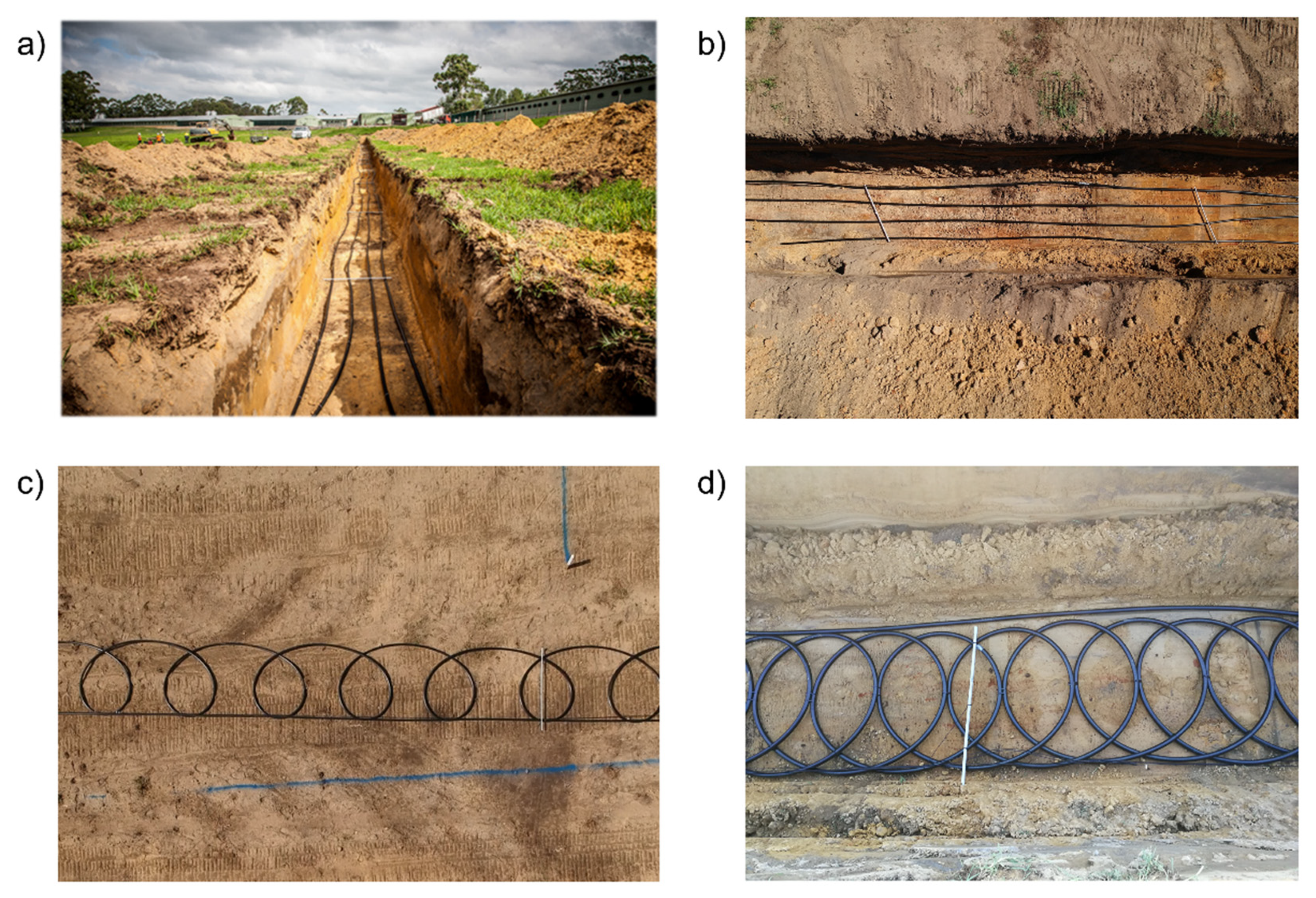
2.2.2. Trench and Pipe Configurations

To study the impacts of different pipe configurations on the performance of horizontal ground heat exchangers, an experimental site with twelve trenches (8 trenches were 75 m long and 4 trenches were 38 m long; all were at a depth of 1.5 m) was used. Each trench/loop consisted of HDPE pipes (with a length of 300 m) with an outside diameter of 32 mm (inner diameter of 26 mm; SRD11). Together, these made up a total pipe length of 4.8 km, excluding the header pipes.

The twelve trenches were placed in groups of four trenches. The first four trenches contained horizontal straight pipes, which consisted of four parallel pipes with a 30 cm spacing between each pipe in a 1.2 m wide, 1.5 m deep, and 75 m long trench; 3.5 m of space was left between each trench. The slinky pipes had a loop diameter of 0.9 m and a loop pitch at 1.37 m, which caused them to have the same pipe length in the same length of trench as the horizontal pipe (four metres of pipe in one metre of trench). These pipes were also buried at a depth of 1.5 m within a 75 m long trench, with a spacing of 3.5 m between each trench. By comparing the performance of the slinky trenches and the horizontal trenches, the impacts of the different pipe layouts on the performance of the horizontal ground heat exchangers under rural industrial conditions could be studied. Lastly, the dense slinky pipes—with a diameter of 0.9 m and a loop pitch of 0.46 m—caused this configuration to have twice the pipe length in the same length of trench in comparison with the previous two configurations (eight metres of pipe in one metre of trench). The trench spacing remained consistent with that of the other configurations (3.5 m). By comparing the performance of these two types of slinky trenches, the impacts of the different pipe densities on the performance of the horizontal ground heat exchangers under rural industrial conditions could be studied. The details of these configurations are shown in Figure 3.

2.2.3. Other Parameters

The model used in this research was based on the typical weather and ground conditions in Peats Ridge, NSW, Australia, as well as the material properties used, which are presented in

Table 2. Material properties.

Parameter	Value(s)	Unit	Description
λground	1.0, 1.5, 2.5	W/(mK)	Effective thermal conductivity of the ground
ρground	2000	kg/m3	Density of the ground
Cp ground	1480	J/(kg·K)	Specific heat capacity of the ground
Tundisturbed	16.1	°C	Undisturbed ground temperature
λfluid	0.582	W/(mK)	Thermal conductivity of the carrier fluid
ρfluid	1000	kg/m3	Density of the carrier fluid
Cp fluid	4190	J/(kg·K)	Specific heat capacity of the carrier fluid
Qfluid	0.42	L/s	Flow rate of the carrier fluid

. The dimensions and geometries used for the models of the GHEs were typical for the region, and they are depicted in Figure 4. It should be noted that while typical GSHP systems include a field with multiple GHEs, in this work, each simulation focused on one single GHE to isolate the effects of the separation of pipes within the GHE from the thermal interference that may arise from adjacent GHEs.

2.2.4. Initial and Boundary Conditions

1

The initial ground and GHE temperatures and the far-field boundary temperature, which was equal to the undisturbed ground temperature, were modelled here as either a uniform temperature (16.1 °C in the experimental field) or as a time- and depth-varying temperature according to Baggs’ adjusted empirical formulations [40]:

T = 16.1 (°C)

(6)

or:

$$T(z,t)=(T_g)+1.07k_v{A}_s\mathrm{Exp}[-0.0031552z{\left(\frac{1}{\alpha }\right)}^{0.5}\left]\times \cos \right[\frac{2\mathsf{\pi }}{365}((t-t_0-0.183355z{(\frac{1}{\alpha })}^{0.5}]$$

(7)

2

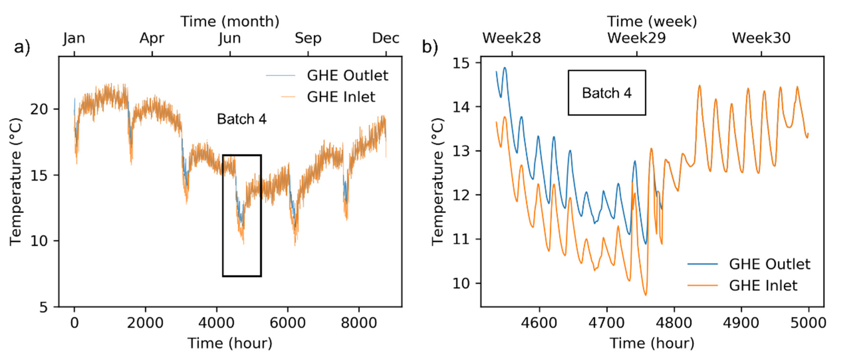
The time-dependent carrier fluid temperature at the inlet, $T_{in\left(t\right)}$, which can be defined as a function of the carrier fluid temperature at the outlet,$T_{out\left(t\right)}$, was obtained from the numerical model and the prescribed time-dependent GHE thermal load, $Q_{GHE\left(t\right)}$. This effectively acts as the transfer function of a heat pump that receives the fluid at a certain temperature and extracts/rejects heat, thus changing the temperature of the fluid, which is reinjected into the ground. The details are illustrated in Figure 4.

$$T_{in\left(t\right)}=T_{out\left(t\right)}-Q_{GHE\left(t\right)}/\left({\rho }_{w}vA{C}_{p,w}\right)$$

(8)

3

A boundary condition of the fluid flow rate at the inlet pipe (s) of about 1.7 L/s or 3.47 m/s was assumed.

$$v_0=3.47 \raisebox{1ex}{$\mathrm{m}$}\!\left/ \!\raisebox{-1ex}{$\mathrm{s}$}\right.$$

(9)

4

A reference atmospheric pressure in the outlet pipe (s) for the purpose of forced convection was assumed:

$$p_0=\mathrm{101,325} \mathrm{Pa}$$

(10)

5

Finally, as shown in Figure 4, there were thermal insulation conditions on both short sides of the field and a symmetric condition on both long sides of the field. The top boundary was set to the outdoor temperature and the bottom to the undisturbed ground temperature (16.1 °C in the experimental field). A symmetric boundary condition was applied at the planes of symmetry, which indicated zero heat flux through the symmetric planes:

$$-n·\left(-{\lambda }_m\nabla T\right)p_0=0$$

(11)

3. Results and Discussion

After the adoption of the methodologies, this section presents the key results and discussions of the study. Ultimately, in this study various simulations were conducted in order to evaluate the performance of a GSHP system with horizontal GHEs under different conditions. To achieve this, first, a validation was performed with consideration of the dimensions of the field and the thermal conductivity of the soil and comparison metrics are introduced. Later, a comparison between different GHE configurations was undertaken. Then, an investigation was performed to evaluate the impacts of different trench separations. Finally, simulations that considered two different effective thermal conductivities, i.e., 1.0 and 2.5 W/(Km), were performed.

3.1. Validation and Comparison Metrics

The performance of the finite element model presented in the previous sections modcan be evaluated by examining the resulting fluid temperatures within the horizontal GHEs. In order to quantify the temperature of the circulating fluid, the average fluid temperature of a pipe loop was used and this was calculated as the average of the temperatures at the inlet and outlet of the fluid in pipes.

To find reasonable dimensions of the soil field, different dimensions of the soil domain were modelled in a steady-state simulation. It was found that larger dimensions of the soil/ground domain lead to more stable and consistent inlet and outlet temperatures of the fluid. The acceptable length and depth of the field were determined to be 120 m (90 m for dense slinky loops, which is 30 m shorter) and 60 m. Apart from the size of the soil field, the mesh size is another factor that impacted the accuracy of the simulation results. Different mesh sizes were tested, and extra-fine mesh was found to be optimal. The time step was also an important parameter when conducting the finite element simulation. The time step to achieve accurate simulation results is related to the spatial resolution, i.e., a denser mesh size requires a smaller time step. In this study, it is found that the time step needed to be set to about 1 h.

Through a comparison against nine-hour field-testing results, this FEM model was validated, and a effective soil thermal conductivity was found to be approximately 1.5 W/(mK) for bets fit. Previous field tests showed an in situ value between 1.8 and 2.2 W/(mK) (thermal needle probe technique on small soil samples). One possible reason for this decrease in the effective soil thermal conductivity was that the soil was not compacted and consolidated enough after excavation and backfilling in the real system tested. The RMSEs of the validation results against inlet and outlet fluid temperatures are shown in

Table 3. Validation parameters. Comparison between numerical and experimental inlet and outlet temperatures.

Thermal Conductivity, W/(mK)	RMSE (Outlet), °C	RMSE (Inlet), °C	RMSE (Temperature Difference), °C
1.5	0.638	0.595	0.058
1.8	0.729	0.685	0.056
2.1	0.798	0.750	0.059
2.5	0.873	0.825	1.543

, showing around 0.6 °C mean error between numerical and experimental results.

Having shown relatively good performance of the numerical model, in the parametric analysis the follows, various combination of input parameters presented in Table 2 are used into simulations with different trench separations while considering three different pipe configurations, i.e., the dense slinky, slinky, and horizontal straight pipe configurations. Later, simulations were conducted to evaluate the importance of the effective thermal conductivity for the performance of ground heat exchangers. As there were a large amount of combinations of input parameters, to be able to perform a large-scale analysis, a single value was used to evaluate the performance of GHEs. This single value captures the difference between simulations of various trench separations for a specific input parameter combinations. As the fluid temperature computed had a yearlong distribution (one value for each hour of simulation), the mean absolute error (MAE) metric in terms of temperature difference was adopted for this study:

$$\overline{T_{MAE}}=\frac{1}{8760}{\displaystyle \sum }_{t=1}^{t=8760}\left|T_{avg,t}^S-T_{avg,t}^s\right|$$

(12)

It is noted that, given the imbalanced heating and cooling loads (Figure 2), increases/decreases in the ground temperature by a few degrees in long periods can be possible. In this study, one-year long simulations were considered to be conservative and appropriate. Moreover, to evaluate the direction of the influence, the average difference was introduced:

$$\overline{T_{diff}}=\frac{1}{8760}{\displaystyle \sum }_{t=1}^{t=8760}(T_{avg,t}^S-T_{avg,t}^s)$$

(13)

The simulation results are illustrated in the next section using this metrics.

3.2. Performance of Horizontal GHEs under Rural Industrial Loading Conditions

In order to better understand of the performance of horizontal GHEs under rural industrial loading conditions, the yearlong simulation responses for the horizontal GHEs in different configurations were analysed first.

As shown in Figure 5, the commonly used horizontal straight GHEs under rural industrial loading conditions resulted in minimum and maximum carrier fluid temperatures of approximately 9.5 and 21.5 °C, respectively, which fit the typical working range of most heat pumps, indicating an adequate initial design.

Corresponding to the six different heating demand cycles shown in Figure 3, there were six operating cycles for the horizontal GHEs within each year. Apart from the operation time, the temperatures of the inlet and outlet were equal and subject to daily and seasonal air temperature variations. A parametric analysis of the different GHE configurations and trench separations is shown in the next section.

3.3. Impacts of the Different GHE Configurations and Trench Separations

To understand the potential influences of the different GHE configurations and trench separations on the performance of a GSHP system, as mentioned in Section 3.2 (Figure 3), three GHE configurations were analysed in this study, i.e., the horizontal straight pipe, slinky, and dense slinky loop configurations. To control the variables, all three configurations had the same pipe length (300 m). The horizontal straight and slinky loop configurations had pipes that were spread over 75 m of trench (4 m of pipe for 1 m of trench). The dense slinky was spread over about 40 m of trench; thus, it was twice as dense (8 m of pipe for 1 m of trench).

Table 4. $\overline{T_{MAE}}$ and $\overline{T_{diff}}$ values for difference configurations and trench separations (using the straight pipe configuration with a 3.5 m separation as reference data).

	$\overline{{\mathit{T}}_{\mathit{M}\mathit{A}\mathit{E}}} (°\mathbf{C})$				$\overline{{\mathit{T}}_{\mathit{d}\mathit{i}\mathit{f}\mathit{f}}} (°\mathbf{C})$
Trench Separation	3.5 m	2.0 m	1.5 m	1.2 m	3.5 m	2.0 m	1.5 m	1.2 m
Straight	N/A	0.43	0.52	0.66	N/A	0.16	0.30	0.46
Slinky	0.47	0.47	0.52	0.63	−0.06	0.08	0.22	0.36
Dense Slinky	1.74	1.87	2.02	2.26	1.74	1.87	2.02	2.26

shows the $\overline{T_{MAE}}$ and $\overline{T_{diff}}$ values for the three configurations with various trench separations and an effective thermal conductivity of 1.5 W/(Km). It was observed that, with the same trench separation, both the $\overline{T_{MAE}}$ and $\overline{T_{diff}}$ for the horizontal straight pipe and the slinky loop were minor. In the dense slinky loop, the $\overline{T_{diff}}$ and $\overline{T_{MAE}}$ were, on average, 1.5 °C lower than in the other two configurations. This was possibly caused by the smaller field size of the dense slinky loop (only 53% of the size of the previous two).

When comparing the $\overline{T_{diff}}$ and $\overline{T_{MAE}}$ values for various trench separations, there was an increasing trend in the carrier fluid temperature when the trench separations were smaller. When the separation was shortened from 3.5 to 1.5 m, the temperature difference increased to about 0.4–0.6 °C. This implies that the trench separation had an impact on the temperature, but it was smaller than the impact of the pipe configuration.

3.4. Impacts of Different Effective Thermal Conductivity

The effective thermal conductivity of the ground was validated as 1.5 W/(Km) based on experimental tests. However, in other, similar practices, this value may vary depending on the geological conditions. Further analysis with two different thermal conductivities, i.e., 1.0 and 2.5 W/(Km), was conducted in order to improve this study’s applicability. The details can be seen in

Table 5. $\overline{T_{MAE}}$ and $\overline{T_{diff}}$ values for difference thermal conductivities with the straight pipe configuration (using the same configuration and separation with a thermal conductivity of 1.5 W/(Km) as reference data).

	$\overline{{\mathit{T}}_{\mathit{M}\mathit{A}\mathit{E}}} (°\mathbf{C})$				$\overline{{\mathit{T}}_{\mathit{d}\mathit{i}\mathit{f}\mathit{f}}} (°\mathbf{C})$
Trench Separation	3.5 m	2.0 m	1.5 m	1.2 m	3.5 m	2.0 m	1.5 m	1.2 m
λground = 1.0 W/(Km)	0.36	0.47	0.36	0.37	−0.12	−0.36	−0.02	0.04
λground = 2.5 W/(Km)	0.42	0.56	0.63	0.75	0.15	−0.01	−0.15	−0.30

.

4. Conclusions

This research developed and validated a new generation of computational models for ground-source heat pump systems with horizontal GHEs. The simulations considered various parameters, including the effective thermal conductivity of the ground, undisturbed ground temperature, properties and flow rates of the carrier fluid, loop configurations, and weather data. Using this model, this study investigated the effects of the trench separation, configuration, and effective thermal conductivity of the soil on the performance of horizontal GHEs under unique rural loading patterns.

First, a yearly performance evaluation of horizontal straight GHEs was conducted under rural industrial loading conditions. The results showed minimum and maximum carrier fluid temperatures of approximately 9.5 and 21.5 °C, respectively, which are within the working range that is typically required by most heat pumps, suggesting an adequate initial design under the unique rural loading patterns.

Next, different trench separations (from 1.2 to 3.5 m) were selected and analysed while considering three different horizontal loop configurations, i.e., the horizontal straight, slinky, and dense slinky loop configurations. These configurations had same length of pipe (300 m) in each trench. The horizontal straight and slinky configurations had the same trench length (75 m), which was about twice that of the dense slinky configuration. The results reveal that there was a minor increase (0.5 °C) in the carrier fluid temperature when the trench separation became smaller. As for the configuration, the dense slinky loop configuration showed an average that was 1.5 °C lower than those of the horizontal straight and slinky loop configurations (which were about the same).

The numerical examples included here suggest that this FEM model can predict the performance of horizontal GHEs reasonably well under the conditions of rural industries’ unique loading patterns. The different trench separations and loop configurations had an impact on the performance of the horizontal GHEs. When the same pipe lengths were used for a given trench length, the impact of the pipe configuration on the performance was minor and sometimes negligible (horizontal straight and slinky examples). Moreover, the trench separation seemed to have less of an impact than the switch from the slinky loop to the dense slinky loop. This indicates that, when land is limited, compromises on the trench separation should be made first rather than changing the loop configuration. Lastly, the impact of the effective thermal conductivity on the performance of the horizontal GHEs was investigated. These results showed that, although there was an impact of effective thermal conductivity on the carrier fluid temperature, this impact was much smaller than those of the GHE configurations and trench separations. Future investigation could continue to perform more tests under different conditions and location to expand the findings of this research.

References

1. Zhou, Z.; Zhang, Z.; Chen, G.; Zuo, J.; Xu, P.; Meng, C.; Yu, Z. Feasibility of ground coupled heat pumps in office buildings: A China study. Appl. Energy 2016, 162, 266–277. [Google Scholar] [CrossRef]
2. Lu, Q.; Narsilio, G.A.; Aditya, G.R.; Johnston, I.W. Economic analysis of vertical ground source heat pump systems in Melbourne. Energy 2017, 125, 107–117. [Google Scholar] [CrossRef]
3. Self, S.J.; Reddy, B.V.; Rosen, M.A. Geothermal heat pump systems: Status review and comparison with other heating options. Appl. Energy 2013, 101, 341–348. [Google Scholar] [CrossRef]
4. Han, C.; Yu, X.B. Performance of a residential ground source heat pump system in sedimentary rock formation. Appl. Energy 2016, 164, 89–98. [Google Scholar] [CrossRef]
5. Yi, M.; Hongxing, Y.; Zhaohong, F. Study on hybrid ground-coupled heat pump systems. Energy Build. 2008, 40, 2028–2036. [Google Scholar] [CrossRef]
6. Lund, J.W.; Boyd, T.L. Direct utilization of geothermal energy 2015 worldwide review. Geothermics 2016, 60, 66–93. [Google Scholar] [CrossRef]
7. Omer, A.M. Ground-source heat pumps systems and applications. Renew. Sustain. Energy Rev. 2008, 12, 344–371. [Google Scholar] [CrossRef]
8. Rees, S. Advances in Ground-Source Heat Pump Systems; Woodhead Publishing: Sawston, UK, 2016. [Google Scholar]
9. Narsilio, G.A.; Aye, L. Shallow Geothermal Energy: An Emerging Technology. In Low Carbon Energy Supply: Green Energy and Technology; Sharma, A., Shukla, D., Aye, L., Eds.; Springer Nature Singapore Pte Ltd.: Singapore, 2018; Chapter 18. [Google Scholar]
10. Demir, H.; Koyun, A.; Temir, G. Heat transfer of horizontal parallel pipe ground heat exchanger and experimental verification. Appl. Therm. Eng. 2009, 29, 224–233. [Google Scholar] [CrossRef]
11. Beier, R.A.; Holloway, W.A. Changes in the thermal performance of horizontal boreholes with time. Appl. Therm. Eng. 2015, 78, 1–8. [Google Scholar] [CrossRef]
12. Johnston, I.W.; Narsilio, G.A.; Colls, S. Emerging geothermal energy technologies. KSCE J. Civ. Eng. 2011, 15, 643–653. [Google Scholar] [CrossRef]
13. Colangelo, G.; Congedo, P.; Starace, G. Horizontal heat exchangers for GSHP. Efficiency and cost investigation for three different applications. In Proceedings of the ECOS2005 18th International Conference on Efficiency, Cost, Optimization, Simulation and Environmental Impact of Energy Systems, Trondheim, Norway, 20–22 June 2005; Volume 2023. [Google Scholar]
14. Congedo, P.M.; Colangelo, G.; Starace, G. CFD simulations of horizontal ground heat exchangers: A comparison among different configurations. Appl. Therm. Eng. 2012, 33–34, 24–32. [Google Scholar] [CrossRef]
15. Esen, H.; Inalli, M.; Esen, M. Numerical and experimental analysis of a horizontal ground-coupled heat pump system. Build. Environ. 2007, 42, 1126–1134. [Google Scholar] [CrossRef]
16. Go, G.-H.; Lee, S.-R.; Yoon, S.; Kim, M.-J. Optimum design of horizontal ground-coupled heat pump systems using spiral-coil-loop heat exchangers. Appl. Energy 2016, 162, 330–345. [Google Scholar] [CrossRef]
17. Tarnawski, V.R.; Leong, W.H.; Momose, T.; Hamada, Y. Analysis of ground source heat pumps with horizontal ground heat exchangers for northern Japan. Renew. Energy 2009, 34, 127–134. [Google Scholar] [CrossRef]
18. Zhou, Y.; Mikhaylova, O.; Bidarmaghz, A.; Donovan, B.; Guillermo, N.; Aye, L. Hybrid geothermal-gas and geothermal-solar-gas heating systems for poultry sheds. In Proceedings of the Zero Energy Mass Custom Home 2018, Melbourne, Australina, 29 January–1 February 2018; pp. 545–554. [Google Scholar]
19. National Famer’s Federation. NFF Annual Review 2014-15; National Famer’s Federation: Canberra, Australia, 2016. [Google Scholar]
20. Australian Bureau of Statistics. 7215.0—Livestock Products, Australia, March 2016; Australian Bureau of Statistics: Canberra, Australian, 2016.
21. Zhou, Y.; Bidarmaghz, A.; Narsilio, G.; Aye, L. Heating and Cooling Loads of a Poultry House in Central Coast, NSW, Australia. In Proceedings of the World Sustainable Built Environment Conference 2017, Hong Kong, China, 5–7 June 2017. [Google Scholar]
22. Webb, M.; Aye, L.; Green, R. Simulation of a biomimetic façade using TRNSYS. Appl. Energy 2018, 213, 670–694. [Google Scholar] [CrossRef]
23. Magnier, L.; Haghighat, F. Multiobjective optimization of building design using TRNSYS simulations, genetic algorithm, and Artificial Neural Network. Build. Environ. 2010, 45, 739–746. [Google Scholar] [CrossRef]
24. Safa, A.A.; Fung, A.S.; Kumar, R. Performance of two-stage variable capacity air source heat pump: Field performance results and TRNSYS simulation. Energy Build. 2015, 94, 80–90. [Google Scholar] [CrossRef]
25. Chargui, R.; Sammouda, H.; Farhat, A. Geothermal heat pump in heating mode: Modeling and simulation on TRNSYS. Int. J. Refrig. 2012, 35, 1824–1832. [Google Scholar] [CrossRef]
26. Chargui, R.; Sammouda, H. Modeling of a residential house coupled with a dual source heat pump using TRNSYS software. Energy Convers. Manag. 2014, 81, 384–399. [Google Scholar] [CrossRef]
27. Trillat-Berdal, V.; Souyri, B.; Achard, G. Coupling of geothermal heat pumps with thermal solar collectors. Appl. Therm. Eng. 2007, 27, 1750–1755. [Google Scholar] [CrossRef]
28. Chong, C.S.A.; Gan, G.; Verhoef, A.; Garcia, R.G.; Vidale, P.L. Simulation of thermal performance of horizontal slinky-loop heat exchangers for ground source heat pumps. Appl. Energy 2013, 104, 603–610. [Google Scholar] [CrossRef]
29. Esen, H.; Esen, M.; Ozsolak, O. Modelling and experimental performance analysis of solar-assisted ground source heat pump system. J. Exp. Theor. Artif. Intell. 2017, 29, 1–17. [Google Scholar] [CrossRef]
30. Tarnawski, V.; Leong, W. Computer analysis, design and simulation of horizontal ground heat exchangers. Int. J. Energy Res. 1993, 17, 467–477. [Google Scholar] [CrossRef]
31. Wu, Y.; Gan, G.; Verhoef, A.; Vidale, P.L.; Gonzalez, R.G. Experimental measurement and numerical simulation of horizontal-coupled slinky ground source heat exchangers. Appl. Therm. Eng. 2010, 30, 2574–2583. [Google Scholar] [CrossRef] [Green Version]
32. Kim, M.-J.; Lee, S.-R.; Yoon, S.; Go, G.-H. Thermal performance evaluation and parametric study of a horizontal ground heat exchanger. Geothermics 2016, 60, 134–143. [Google Scholar] [CrossRef]
33. Dehghan, B.; Sisman, A.; Aydin, M. Parametric investigation of helical ground heat exchangers for heat pump applications. Energy Build. 2016, 127, 999–1007. [Google Scholar] [CrossRef]
34. Simms, R.B.; Haslam, S.R.; Craig, J.R. Impact of soil heterogeneity on the functioning of horizontal ground heat exchangers. Geothermics 2014, 50, 35–43. [Google Scholar] [CrossRef]
35. D’Agostino, D.; Greco, A.; Masselli, C.; Minichiello, F. The employment of an earth-to-air heat exchanger as pre-treating unit of an air conditioning system for energy saving: A comparison among different worldwide climatic zones. Energy Build. 2020, 229, 110517. [Google Scholar] [CrossRef]
36. Bidarmaghz, A. 3D Numerical Modelling of Vertical Ground Heat Exchangers. Ph.D. Thesis, The Unversity of Melbourne, Parkville, VIC, Australia, 2015. [Google Scholar]
37. Barnard, A.; Hunt, W.; Timlake, W.; Varley, E. A theory of fluid flow in compliant tubes. Biophys. J. 1966, 6, 717–724. [Google Scholar] [CrossRef] [Green Version]
38. Lurie, M.V. Modelling and Calculation of Stationary Operating Regimes of Oil and Gas Pipelines; Wiley-VCH Verlag GmbH & Co. KGaA: Weinheim, Germany, 2008. [Google Scholar]
39. Remund, J.; Müller, S.; Kunz, S.; Huguenin-Landl, B.; Studer, C.; Cattin, R. Meteonorm Handbook part II: Theory, Global Meteorological Database Version 7 Software and Data for Engineers, Planers and Education (2018). Available online: http://www.meteonorm.com (accessed on 28 April 2021).
40. Baggs, S.; Baggs, D.; Baggs, J.C. Australian Earth-Covered Buildings; New South Wales University Press: Randwick, NSW, Australia, 1991. [Google Scholar]
Figure 1. Diagram of the hybrid geothermal system for poultry sheds. Each trench is 75 m long and contains 300 m of HDPE pipes (highlighted in red).
Energies 14 03919 g001
Figure 2. Hourly heating demand of the chicken shed: (a) yearly loading pattern showing the six batches; (b) details of these six heating cycles over one year.
Energies 14 03919 g002
Figure 3. Ground heat exchangers in the field: (a) horizontal straight loop in a trench; (b) horizontal straight loop; (c) slinky loop; (d) dense slinky loop.
Energies 14 03919 g003
Figure 4. Detailed configuration of the inlet and outlet pipes.
Energies 14 03919 g004
Figure 5. Outlet and inlet temperatures of the FEM-simulated GHEs: (a) results for one TMY; (b) results for batch 4.(system turned off at about 4800 h, ~12 days of heating in this batch).
Energies 14 03919 g005