Automated Testbench for Hybrid Machine Learning-Based Worst-Case Energy Consumption Analysis on Batteryless IoT Devices

Abstract

Batteryless Internet-of-Things (IoT) devices need to schedule tasks on very limited energy budgets from intermittent energy harvesting. Creating an energy-aware scheduler allows the device to schedule tasks in an efficient manner to avoid power loss during execution. To achieve this, we need insight in the Worst-Case Energy Consumption (WCEC) of each schedulable task on the device. Different methodologies exist to determine or approximate the energy consumption. However, these approaches are computationally expensive and infeasible to perform on all type of devices; or are not accurate enough to acquire safe upper bounds. We propose a hybrid methodology that combines machine learning-based prediction on small code sections, called hybrid blocks, with static analysis to combine the predictions to a final upper bound estimation for the WCEC. In this paper, we present our work on an automated testbench for the Code Behaviour Framework (COBRA) that measures and profiles the upper bound energy consumption on the target device. Next, we use the upper bound measurements of the testbench to train eight different regression models that need to predict these upper bounds. The results show promising estimates for three regression models that could potentially be used for the methodology with additional tuning and training.

1. Introduction

The Internet-of-Things (IoT) is an emergent technology which consists of internet-enabled devices in a network that are capable of sensing, processing and performing autonomous actions through communication. An IoT system comprises of the distributed software or ’intelligence’ that is deployed across the computational devices or nodes in the (heterogeneous) network. The computation is performed on network nodes that are located in the cloud (i.e., server infrastructure) to the edge (e.g., sensor nodes, actuators, etc.) of the network. IoT applications range from intelligent lighting and Heating, Ventilation and Air Conditioning (HVAC) control at home to predictive automotive maintenance where the system will make an appointment at the garage and order new parts for your car based on the data of the numerous sensors monitoring the car’s behaviour. These systems are able to sense and interact with their environment through sensors and actuators, respectively. For example, a humidity and CO${}_2$ sensor will measure the air quality and perceive a state of the room. Depending on that state, the room’s climate control can decide to open a window to cool down the room and/or actuate the heater knob. By adding additional sensors and external data sources, such as an infrared presence sensor and a digital room booking calendar, the system will be able to make more optimal decisions based on current and future occupancy of the room. The application becomes ’smarter’ as more data and devices are available. In 2018, an estimated total of 22 billion IoT devices were globally in use and it is expected that these numbers will grow to 50 billion by 2030 [1] with a still growing market [2].

Many IoT devices are small or mobile nodes that are operated by batteries, as providing outlet power to the vast number of devices on different and/or remote locations is not feasible. Nevertheless, these battery-operated devices come with a high cost. Batteries have a large impact on the environment because they contain heavy metals that impact health and contribute to the greenhouse emissions during the exploitation of the minerals and production [3,4]. Furthermore, the limited lifespan and energy capacity of batteries require regular servicing of these devices on site which comes with high operational costs. When the number of IoT devices reach 50 billion, we will need up to 1 trillion batteries to power those devices. With an optimistic lifespan of 10 years, a total of over 274 million batteries need to be replaced every day that end up in toxic waste [5]. As a result, energy is a hard-constrained resource for these devices.

An alternative to the relative short-lasting and environmentally harmful batteries is the evolution to batteryless devices [6]. The batteries in these devices are replaced by an energy harvesting circuit harnessing environmental sources, such as solar-, kinetic- or Radio Frequency (RF)-energy [7], and a (super)capacitor storage element. A capacitor has a longer lifespan compared to batteries due to the larger number of recharge cycles it is able to handle [8]. Supercapacitors in particular have higher power density (W/kg) characteristics and charge much faster than batteries. However, the energy density (Wh/kg) of these storage elements is significantly lower [9]. Therefore, the available energy is even more scarce for batterless devices. In order to operate within these constraints, the software needs to schedule its tasks while taking the available produced and stored energy into account.

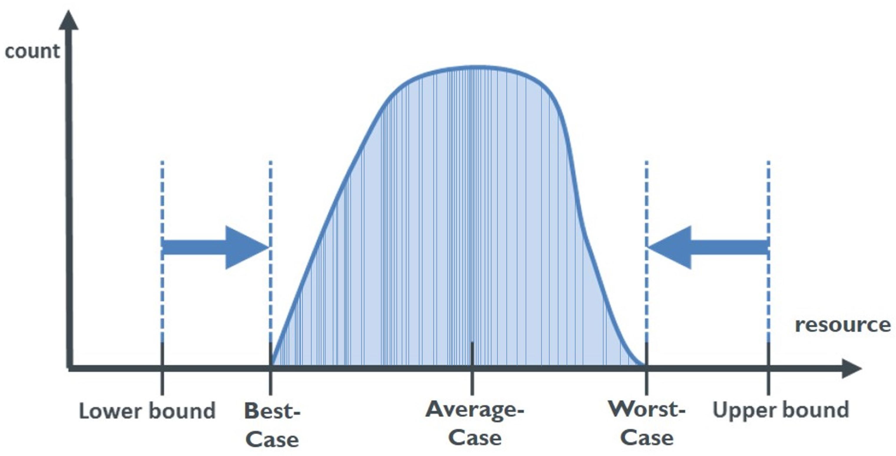
Cyber–Physical Systems (CPS) are software-controlled machines that interact with their environment and have real-time behaviour. In these real-time operating systems, a scheduler is used to plan and execute a set of software tasks that has timed constraints, such as periodicity or hard deadlines [10]. For each of these tasks, the scheduler needs insight in the behaviour of the task, e.g., the execution time. The execution time, or resource consumption in general, of a task is not a single value, but a distribution, as shown in Figure 1. When designing a software-controlled system with hard constraints, the worst-case scenario of a task should always lie within the imposed boundaries of that system. For example, in hard real-time systems the approximation or upper bound of the Worst-Case Execution Time (WCET) needs to be determined for each task. This upper bound is then used by the scheduler to schedule each task within its deadlines.

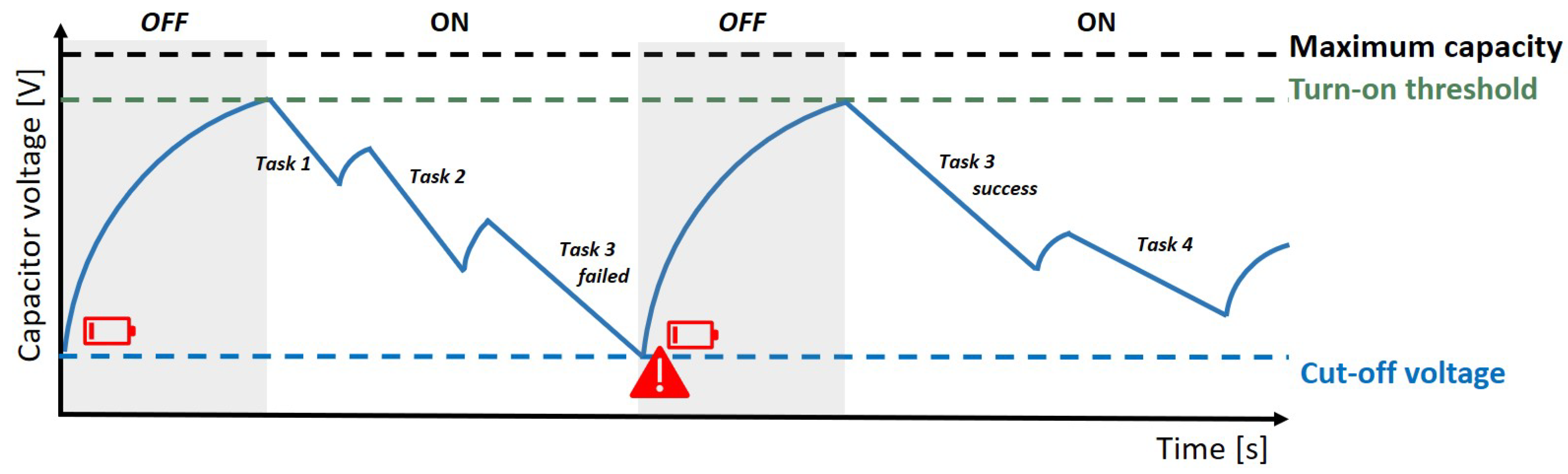
In the state-of-practice, most schedulers in batteryless devices have no knowledge of the available energy and take a best effort approach to schedule all tasks [6,11] as illustrated in Figure 2. Therefore, tasks may fail when the voltage has dropped below the cut-off voltage before they are completed. Failed tasks need to be resumed later when the capacitors are back at full charge. In the example of Figure 2, all tasks are scheduled one after the other. The execution of Task 3 is interrupted, however, as the capacitor has dropped below the cut-off voltage. After the capacitor is above the turn-on voltage, the failed Task 3 is retried. As a result, valuable energy is lost during the failed task execution that could have been used for another task, or the task could have been finished successfully if the device had waited until enough energy was available in the capacitor. Furthermore, failing tasks are prone to miss their execution deadline resulting in corrupt, incomplete or obsolete data and actions. Current research is being conducted to create schedulers that are aware of energy availability [12,13]. This will allow the scheduler to turn into a low-power mode to avoid rescheduling failed tasks due to power loss, and eventually lowering the chances of missing execution deadlines. Nonetheless, the scheduler requires insight in the Worst-Case Energy Consumption (WCEC) of each task in order to schedule them, which are not trivial to obtain.

In this article, we propose a hybrid analysis methodology to gain insight in the WCEC of a software task on a given hardware platform. Firstly, we outline the state-of-the-art of WCET analysis and present our approach to estimate the WCEC in Section 2. Secondly, Section 3 describes the implementation of an automated testbench to acquire accurate energy measurements from annotated code blocks. These measurements are then used to train WCEC estimation models that are presented in Section 4. Finally, preliminary results from these models are evaluated and discussed in Section 5.

2. Background

In this section, we look at related work and methodologies used in the domain of WCET analysis and apply these techniques on other resources, such as energy, execution time, data throughput, memory usages, etc. Our long-term goal is to obtain an overall Worst-Case Resource Consumption (WCRC) analysis that describes general approaches to determine the worst-case behaviour of different system resources. In this paper, we use insights from the field of WCET analysis to propose a new hybrid approach to tackle the WCEC analysis using machine learning.

2.1. Worst-Case Resource Analysis

In order to determine the energy consumption, three main approaches exist. First, the static analysis will approximate the upper bound of the WCEC by creating a mathematical model of the software and interactions with the systems’ hardware. This methodology provides accurate results depending on the model. Creating a sound mathematical representation of the system and its internal states makes this solution computationally very expensive or even infeasible to solve. This is due to the unpredictability of hardware states and anomalies introduced by the hardware components, such as cache memory, branch prediction, multi-stage pipelines, etc.

A second approach is the measurement-based methodology. The resource consumption of the application is measured by running the code multiple times on the target platform with different input sets. The resulting distribution of the measurements provides three boundaries: best-case, average-case and worst-case, as shown in Figure 1. The number of measurements is determined by the analysis cost and effort that is affordable to perform. For complex systems, it becomes infeasible to achieve full coverage of all states. Therefore, the limited number of measurements will never guarantee that the real worst-case is detected. A safety margin is therefore added to the measured worst-case, or upper bound, to minimise the risk for underestimating the real worst-case consumption [14]. The upper bound should always be kept higher than the actual worst-case, but as a result will introduce pessimism to the design. The goal is to get the upper bound as close as possible to the worst-case in order to minimise this pessimism.

The third approach, we use in our research [15], is the hybrid methodology, which is a combination of the analysis techniques above. By splitting the code into smaller components, or ‘hybrid blocks’, we are able to create a balance between the computational complexity and accuracy. Each hybrid block contains a single trace of consecutive instructions that has one entry and one exit point. These blocks have a similar functionality to ‘basic blocks’, but the size of a hybrid block may vary from a single instruction up to entire code sections or functions depending on the target accuracy and complexity we want to achieve. The first stage consists of determining the worst-case resource consumption of the blocks by measurement. The second step is to statically combine the results to gain insight in the worst-case consumption.

The research on hybrid WCRC analysis has been integrated within the Code Behaviour fRAmework (COBRA) tool which we developed. This framework is a collection of tools to examine the behaviour of code on different computing platforms [15]. The current implementation provides insights for embedded developers in three categories: WCRC analysis, scheduler optimisation [16] and design pattern-based performance optimisation for multi-core processors. In previous research, we implemented the hybrid methodology to estimate the WCET on embedded devices [15]. The results showed a reduction in effort while keeping sound WCET predictions. However, the measurements of the hybrid blocks still required high effort to compile and run the source code on the target platform. In addition, this approach is only applicable if the target platform is available to perform analysis on.

2.2. Early Stage Analysis Using Machine Learning

Measurements on the physical device require long and high effort to accomplish, and can only be performed in the validation stage of the design. A better approach would be to gain insight early on in the development process without tedious measurements to ‘fail fast’, so that the developer has the opportunity to fix the design much faster and reduce costs. Previous research has proposed new methodologies to gain early insight in the domain of execution time. Altenbernd et al. [17] used a linear time model with Simulated Annealing (SA) algorithms that translates code into basic instructions for which the timing is determined. This technique is extended in other research by using machine learning. Bonenfant et al. [18] approximated the WCET by training a neural network using worst-case event counts which are matched to a WCET estimate for the target architecture. In [19], we extended the hybrid analysis methodology with machine learning to predict the WCET of hybrid blocks. A list of software features was used as input to train regression models for a fixed hardware platform. The research of Bachard et al. [20] has extended on the hybrid analysis principle with machine learning on a lower level, i.e., machine code, to incorporate cache behaviour and tackle the training data issue by automatically generating code samples. In this paper, we focus on adopting these techniques used in the domain of WCET analysis to obtain estimations for WCEC.

2.3. Worst-Case Energy Consumption Analysis

The base formula to calculate the electrical energy (Joule: J) is the integral of the power draw over a time interval: $E={\int }_{t=0}^{T}V\left(t\right)I\left(t\right)dt$. For the WCEC, we are interested in finding the maximum amount of energy a given piece of code will consume on the target platform. Therefore, we need to find the path in the code which would result in the highest energy consumption. One could think that the WCEC is equal to the longest execution path, as energy is the power draw over time. However, this naive conclusion is definitely not sound. In the context of execution time, the longest code trace, for example, does not guarantee the worst-case scenario. This is caused by timing anomalies that are introduced by the hardware [21], such as cache misses, out-of-order execution, etc. [22]. These anomalies also apply for the energy consumption. The total energy consumption is determined by instruction-specific silicon that is activated during the different stages of the instruction pipeline and performance enhancing hardware, such as cache memory and branch prediction. There is no guarantee that the longest execution path results in the highest energy consumption or visa versa. Experimental research has showed that no direct correlation exists between execution time and energy consumption [23].

The power draw of the hardware consists of two parts: static and dynamic power dissipation [23,24]. The static component is the power that the hardware dissipates or ‘leaks’ when it is turned on in a stable environment, e.g., constant voltage, clock frequency and temperature, without considering the state or in- and outputs of the system. The energy consumption of the static power component is therefore directly proportional to the execution time of the program in an ideal environment. The dynamic component comprises the power dissipation of the activity on the hardware due to the code, changing states and I/O on the system. The dynamic power usage in the processor is the result of the switching and retaining the state of the circuit logic, such as registers, data buses, clock tree, Arithmetic Logic Unit (ALU), etc.

According to Morse et al. [24], determining the dynamic power consumption is not a trivial problem. For execution time analysis, the time can be quantized to the number of clock cycles it takes to execute. This approach results in a set of discrete execution time possibilities. When we shift to energy, the power consumption is added to the equation. Power cannot directly be quantized as execution time to the clock period, but is correlated to the number of transistors and their probability to change depending on the data for each operation. The complexity to statically calculate the energy consumption rises tremendously as the consumption for a single instruction varies on the Hamming distance, i.e., number of flipped bits, of each register during operation and thus, is dependent on the data input and its state. The state space of possible switches in hardware that we need to keep track of during analysis is equal to the powerset $2^S$ with $\left|S\right|$ equal to the number of transistors in the processor. Therefore, Morse et al. [24] concluded that this ‘Circuit Switching Problem’ is an NP-hard problem intractable to solve. While some research has claimed that the dynamic component of circuit switching does not contribute a significant part in the total energy consumption [23,25], other researchers have noticed that the switching due to data input has a substantial impact of the observed consumption [24,26] when solely looking at the energy consumption of the processor. Nonetheless, the energy consumption of the processing unit is sometimes only a fraction of the total energy consumption of the embedded systems depending on its peripherals [27], such as sensors, and most definitely wireless transceivers. The fluctuations in the energy usage of instructions due to data will become so small that it could be perceived as noise.

In the state-of-the-art, we see lots of research on creating energy models of embedded processors, such as the ARM Cortex-M, XMOS xCORE, AVR, LEON3, etc. A first approach by Tiwari et al. [28] proposed a measurement-based analysis technique to quantify the power usage per instruction and the cost of switching between instructions. The model is then able to estimate the energy consumption of a code trace. This model was further extended by Steinke et al. [29] by including the switching activity on the data buses of the processor as the toggling bits take a major role in the energy consumption of the processor. In the EU ENTRA project [30], they investigated an energy transparent methodology for energy-aware development by using static analysis techniques for energy consumption estimations at compile time. In a first stage, they applied the static approach on the instruction (Instruction Set Architecture—ISA) level [31], and later extended it on the block level of the LLVM compiler [32]. All these methodologies focus on estimating the energy consumption, but are not looking at WCEC.

In the work of Jayaseelan et al. [23], they pointed out the need of taking energy constraints into account for mission critical battery-operated systems. In order to provide these guarantees, we need insight into the WCEC behaviour of computing tasks on the system. Compared to the work mentioned in the previous paragraph that focuses on average-case energy consumption, the research of [23] presents a static analysis approach that estimates the WCEC. Their methodology starts with estimating an upper bound for each basic block in the code. This upper bound is the sum of static leak power and the dynamic energy consumption of each instruction. Next, an Integer Linear Programming (ILP) solver is used to find the path with the highest energy consumption based on the Control Flow Graph (CFG) of the program.

Research by Wägemann et al. [33] uses the ILP technique combined with symbolic execution and genetic algorithms to create a hybrid tool 0g for WCEC analysis. Based on requirements, the tool selects the best approach to limit the analysis duration, and if it should under- or over-approximate the upper bound. The static analysis tools are able to use absolute energy models that provide exact numbers on the energy cost of an instruction. However, creating such a model is difficult to achieve due to non-deterministic behaviour of the hardware, or not having access to the implementation details of the architecture. On the other hand, the 0g tool is able to estimate WCEC based on relative energy models with genetic algorithms to determine valid input sets that trigger the worst-case path, but this will not provide absolute WCEC. These input sets are used to perform physical measurements on the device to obtain a WCEC upper bound.

In

Table 1. Overview of different methodologies from related research in comparison to our work. R1: Altenbernd et al. [17], Bonenfant et al. [18], Huybrechts et al. [19] and Bachard et al. [20]; R2: Tiwari et al. [28]; R3: Steinke et al. [29]; R4: EU ENTRA project [30]; R5: Jayaseelan et al. [23]; R6: Wägemann et al. [33]; R7: our work; ${}^1$ Hardware model is required; ${}^2$ Average-Case Energy Consumption; ${}^3$ LLVM’s intermediate representation; ${}^4$ Fallback strategy if the hardware model is not available; ${}^5$ ARTIST2 Language for WCET Flow Analysis.

	R1	R2	R3	R4	R5	R6	R7
Resource	WCET	WCEC	WCEC	ACEC ${}^2$	WCEC	WCEC	WCEC
Approach	Static/ Hybrid	Measur.	Hybrid	Static	Static	Hybrid	Hybrid
Target Platform	All	All	+/− ${}^1$	+/− ${}^1$	+/− ${}^1$	All ${}^4$	All
Code Level	ALF ${}^5$/ ISA/ Source	ISA	ISA	ISA/ LLVM ${}^3$	ISA	LLVM ${}^3$	Source
Machine Learn.	Yes	No	No	No	No	No	Yes
Early Stage Predictions	Yes	No	No	No	No	No	Yes

, we present a summary of the related research we discussed in this paper and how our proposed work is novel in comparison.

3. Materials and Methods

The goal of this research was to introduce machine learning techniques to approximate the WCEC. As creating a sound energy model is an NP-hard problem due to the ‘Circuit Switching Problem’ [24], we want to study the capability of machine learning to make an abstraction of the hardware and learn its behaviour. In this section, we will discuss the experimental setup we created, on which we will train prediction models. Next, we look at the regression models we selected for this first experiment. Finally, the practical implementation of our hybrid methodology with an automated testbench is presented.

3.1. Experimental Setup

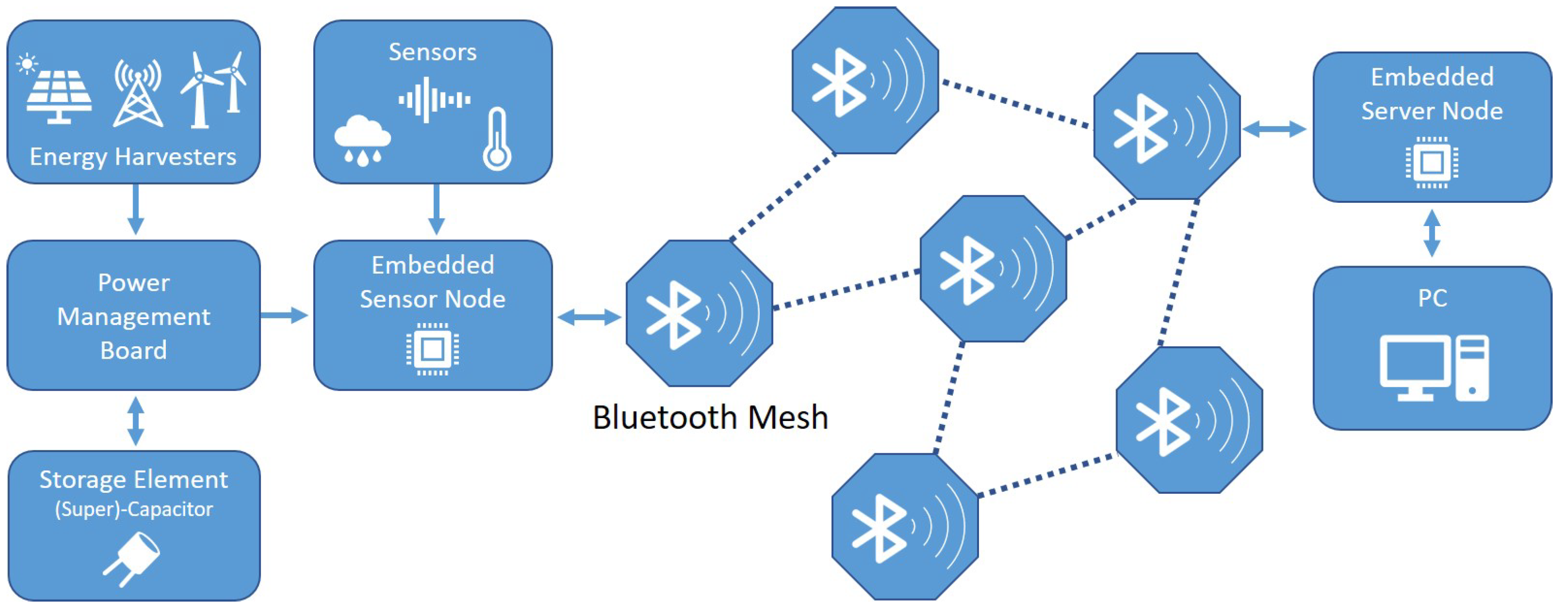
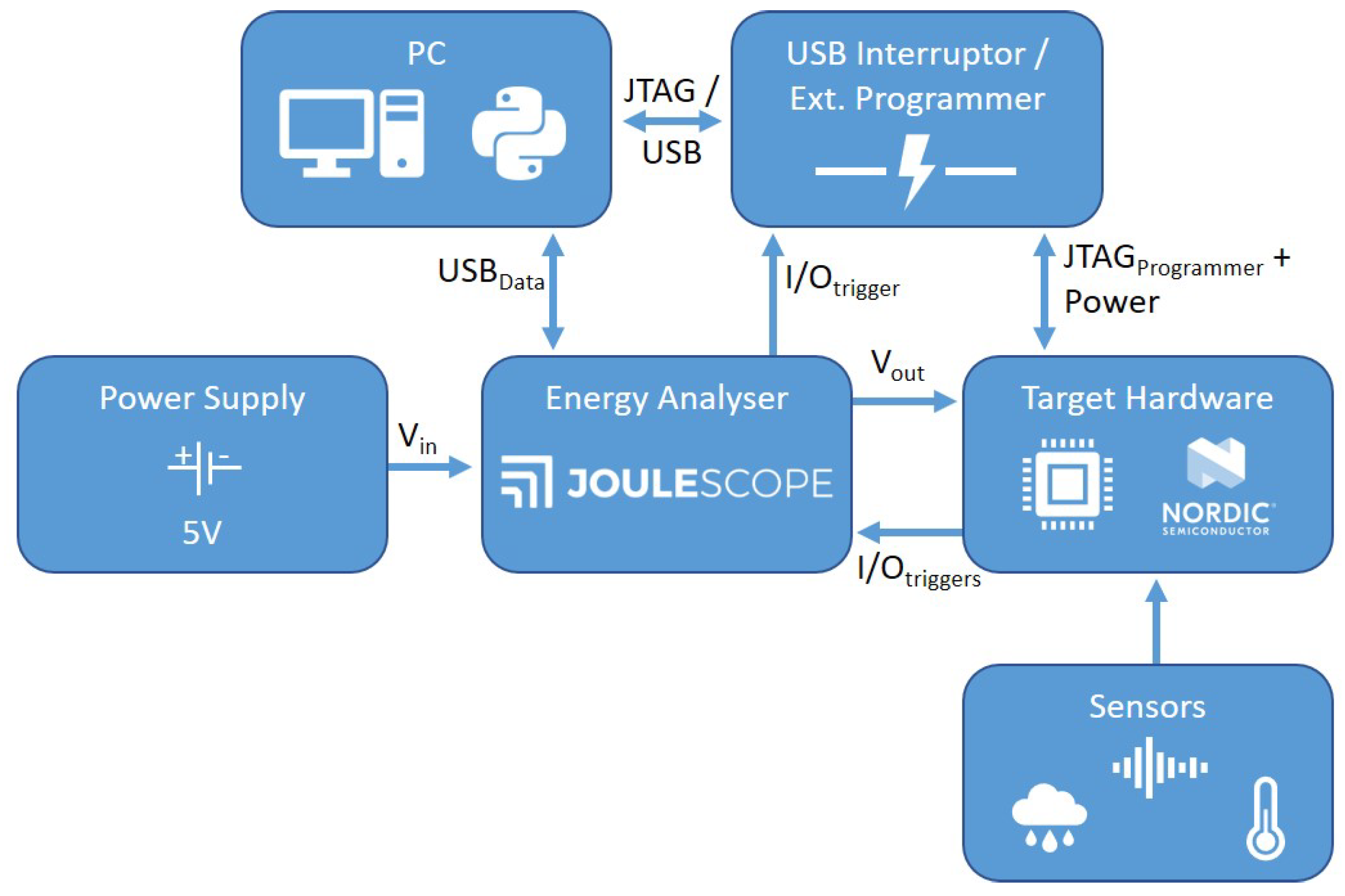
For this experiment, we use a small IoT setup that consists of embedded controllers in a Bluetooth mesh network. The clients are batteryless nodes equipped with sensors, e.g., temperature, to monitor the environment. Each remote sensor node has a power management board with a supercapacitor to store the energy and an energy harvesting device, such as solar panels. Each client has to schedule a set of tasks with a limited energy budget. These tasks vary from reading sensor values, performing small calculations with the data, storing intermediate data to the internal flash memory, and transmitting the data to a server node in the mesh network. A schematic overview of the system is illustrated in Figure 3. The target embedded controller used in our setup is the Nordic nRF52 development kit board with an nRF52832 System-on-Chip (SoC) that is built on top of an ARM Cortex-M4 Central Processing Unit (CPU) [34]. The onboard energy-aware software scheduler requires a schedule with the requested task’s periodicity, and a list of the WCET and WCEC predictions of each schedulable task. These predictions are determined before final deployment on the hardware and provided in a configuration file to the scheduler. The offline profiling of each software task is performed by an automated testbench (Section 3.4) we created for the COBRA framework (Section 3.3) with the use of machine learning (Section 3.2).

3.2. Machine Learning

In previous research [19,35], we used machine learning techniques to estimate the WCET. These models were created with the concept to predict the worst-case based on those events and interactions that would result in the highest execution time path. Soft- and hardware related attributes could be used to describe the behaviour of the code on the platform. Machine learning has the ability to find correlations in data and learn complex system behaviour from it. We believe that machine learning could provide a valuable solution in early stage WCRC analysis by making abstraction of the complex interactions and behaviour of the software with the system hardware.

The machine learning method of Bonenfant et al. [18] uses event counters to characterise the WCET behaviour. However, this approach creates a high abstraction of the complete source code base and, therefore, loses valuable flow information. A similar approach has been examined by Griffin et al. [36] with performance monitoring counters as attributes for Deep Learning Neural Networks in multi-core processors. The results are promising with small underestimated upper bounds. Nevertheless, the methodology still requires physical measurements on the platform to acquire the performance counters and the single core performance. By using the machine learning estimation model to replace the measurement-based layer in the hybrid methodology, we reduce the analysis effort, and have the opportunity to characterise the source code on the block level to incorporate code flow information in the static layer and reducing the classification complexity of the estimation model.

The WCEC behaviour depends on the soft- and hardware of the system. For this paper however, we will only focus on the software related attributes to reduce the complexity of these first experiments. These software attributes are numeric representations of a hybrid block’s code that are used as feature input for the machine learning models.

Table 2. Code attribute types from the hybrid blocks used as input features for the prediction models.

Attribute	Description
Additive	Number of add/subtract operations. [+, ++, +=, -, –, -=]
Multiplicative	Number of multiplication operations. [*, *=]
Division	Number of division operations. [/, /=]
Modulo	Number of modulo operations. [%, %=]
Logic	Number of logic operations. [&&, ||, !]
Bitwise	Number of bitwise operations. [&, &=, |, |=, ⌃, ⌃=, ~]
Assign	Number of assignments. [=, +=, ++, -=, –, *=, /=, %=, <<=, >>=, &=, ⌃=, |=]
Shift	Number of shift operations. [>>, <<, >>=, <<=]
Comparison	Number of comparison operations. [==, !=, <, <=, >, >=]
Return	Classification if a return statement is present.
Evaluation	Number of logic evaluation statements. [if, switch, ?]
Iteration	Number of iteration statements. [while, for, do-while]
Local variables access	Number of accesses (read/write) to local variables.
Local array access	Number of accesses (read/write) to local arrays.
Global variables access	Number of accesses (read/write) to global variables.
Global array access	Number of accesses (read/write) to global arrays.

lists the software attributes that are extracted from each hybrid block. The selected features are picked in previous experiments based on visual inspection of hybrid blocks and identifying those code related features that characterise the code execution (e.g., actual instructions) and have a significant impact on the hardware [22]. These features are automatically extracted from source code [19] and are, therefore, related to the C-code syntax. Most features are based on the number of occurrences per classified operation type. The size of the generated hybrid blocks is small and the feature list is kept limited to reduce the complexity in this first attempt. Nevertheless, this list can be further expanded and improved on in future research by employing feature engineering techniques [37,38], such as correlation analysis between features and feature extraction strategies [39].

In the hybrid analysis methodology [15], the WCEC of each block is first determined by empirical analysis on the physical hardware and then statically combined. However, we aim to reduce the analysis effort by replacing the physical measurements with a machine learning estimation layer. The estimation layer takes the set of features of Table 2 as input and returns an upper bound prediction of the WCEC. A regression technique is particularly suitable for this problem statement because the numeric features are used as predictor inputs to find a numeric relation with a single output variable (i.e., worst-case upper bound) [39]. Eight different regression models are selected for comparison in this experiment, as listed in

Table 3. Regression models selected for the experiment as WCEC estimators.

Linear Regression	Polynomial Regression (3rd Degree)
Decision Tree Regression	Random Forest Regression
Support Vector Reg. (Linear Kernel)	Support Vector Reg. (RBF Kernel)
K-Nearest Neighbours Regression	Ridge Regression

. Each of these models are implemented in Python with the Scikit-Learn framework [40].

The regression models have to be trained with annotated examples. A supervised learning paradigm is applied as we expect the estimation model to return an absolute value for the upper bound. Creating a dataset for training and validation requires us to generate a large database of hybrid blocks with the extracted features and associated upper bounds. The annotated WCEC estimates are used during training to calculate the prediction error to minimise the cost function, and to verify the performance of the model during the validation step. In order to create such database of annotated blocks, we use the TACLeBench as a code base to generate hybrid blocks for training.

The TACLeBench is a benchmark project of the TACLe community to evaluate timing analysis tools and techniques in order to compare their performances [41]. This benchmark is an open source collection of over 50 benchmark programs composed from different research groups and tool vendors [41]. The advantage of this benchmark suite is the collection of benchmark applications that are fully self-contained in only one source file without any system-specific dependencies. Therefore, each program is easily deployable on different hardware architectures. Additionally, all code is annotated with different flow facts [41]. These flow facts provide hints on the entry point of the application and the minimum/maximum number of iterations for each loop, i.e., loop bound. These flow facts and the self-contained code significantly help the automated block generation process with the COBRA tool.

3.3. COBRA Framework

The hybrid WCEC analysis methodology comprises of splitting the source code into smaller blocks, measuring or estimating the worst-case behaviour of those blocks and lastly, statically combining all block results to a final upper bound estimation of the total program. Performing all these steps are tedious and time consuming. A set of software tools have been developed to facilitate the analysis process. All tools are now integrated as the Hybrid Program Analyser (HPA) addition to the COBRA framework [15].

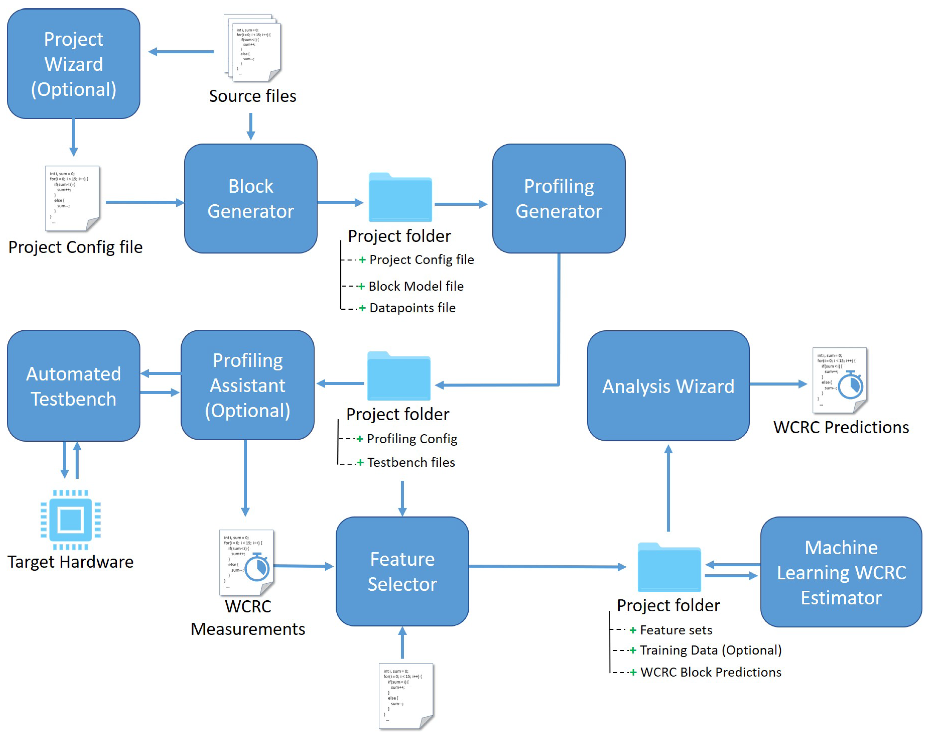
The HPA extension of the COBRA framework is a chain of tools that execute each step sequentially as illustrated in Figure 4. The functional operation of the framework is based on project files. In order to perform an analysis on a code project, one needs to define a Project Configuration file that contains the file locations of the source code and several configurations of the desired analysis strategy, such as block splitting and Target Hardware configurations. This configuration file is stored in a dedicated Project folder that will contain all generated files of the project by all the COBRA tools. These project files are passed through the chain and, therefore, allow the user to interrupt and continue operation between steps, or change settings of one step in the chain without having to rerun the process from the start. The Project Configuration file is an XML file which the user is able to write on its own. Nevertheless, we have created an easy to use tool that assists the user in creating and managing these project files with the Project Wizard.

The first step in the hybrid analysis is the creation of the hybrid blocks by the Block Generator. These blocks contain a section of the source code. Each block is statically analysed for instruction classification, e.g., loops, jump instructions, etc., and extraction of flow facts and variables. All this information is exported into the Block Model file in the Project folder. This block model is the base for all operations in the COBRA-HPA toolchain. The Block Generator has different strategies to split the code into hybrid blocks. An elaborated discussion on the creation of these hybrid blocks and the block model representation is presented in [15].

The second step in the process is the generation of testbench code for each hybrid block. A testbench is a template code file that contains the source code of the hybrid block to be profiled. The code file is hardware agnostic with a four-step profiling methodology. These steps are specifically defined for the Target Hardware and imported in the testbench at compile time in the Profiling Assistant. The profiling process contains an initialisation, data setup, testbench run and finally, epilogue step. In order to create compilable testbench code, the Profiling Generator performs a dependency analysis to determine which variables are used, their scope and if they are declared and defined inside the block or not. If a variable is declared outside the scope of the block’s code, the Profiling Generator will declare them in the testbench code on the same scope level as in the source files. Next, it will try to find valid input sets for these variables, such as defined constants or explicit values deduced from preceding blocks in the control flow. The user is able to provide valid input sets when no values can be found. The input sets are used during profiling to test different code paths and states for worst-case behaviour. All testbench code and dependency analysis results are finally exported to the Project folder.

The third step is the physical measurement of the code behaviour on the hardware with the Profiling Assistant. This step is used to create training and validation data for the prediction models and therefore, is optional when using a trained model to predict the WCRC. The Profiling Assistant automates the entire process of profiling all blocks one after the other on the Target Hardware. Based on the index file of the Profiling Generator, the tool will collect the testbench, source files and hardware configuration to compile a binary file for the target platform. Next, it will flash and restart the board to run the profiling procedure. The COBRA-HPA platform supports execution time and energy measurements. Depending on the Target Hardware capabilities, the assistant will select an appropriate strategy to measure the consumption usage, e.g., a Tic-Toc cycle counter. For the energy measurements on the Nordic sensor node as described in Section 3.1, we created an automated testbench that works together with the Profiling Assistant to perform energy measurements on the physical hardware. This testbench is presented in more detail in Section 3.4. Lastly, all measurements are accumulated by the Profiling Assistant and statistics are calculated, such as the worst-case upper bound. The upper bound measurements are stored in the Project folder to label each block datapoint for training and validation purposes of the Machine Learning WCRC Estimator.

The fourth step of the machine learning-based analysis is the extraction of software features from the hybrid blocks. The Feature Selector uses token- and semantic-based rules to acquire the described features of Table 2. The extraction definition for each desired feature is declared in the Feature Detector Configuration and comprises one or more detector types that are chained together. These detectors are built on top of the ANother Tool for Language Recognition (ANTLR v4) framework [42] and uses a grammar definition file to split code into tokens with semantic rules. The result is a parse tree that is traversable as a means for semantic composition of each instruction in the code. The Feature Selector currently has seven detector types that can be classified in three distinct classes:

• Token-based detectors count each occurrence of basic tokens and map them to a feature, e.g., ’+’, ’++’, ’if’, etc.;
• Context-based detectors check if a syntactic rule is in the context of the traversed node in the parse tree, e.g., pointer, unary operator, etc.;
• Collection-based detectors provide basic set operations on the output of other detectors, e.g., accumulation of sets, union between sets, etc.

The extracted features are exported to a formatted Comma-Separated Values (CSV)-file in the Project folder. This file will be used by the machine learning model as an input that describes the source code at a higher abstraction level.

The fifth step is the Machine Learning WCRC Estimator which provides an upper bound prediction of the WCRC as described in Section 3.2. In this experiment, we will use the regression models of Table 3. These models will only provide estimates for each block individually and, therefore, require us to combine them statically into one final upper bound prediction in a final step. In related research, we performed experiments with deep neural networks that were able to perform the accumulation step for us [35].

The final step in the toolchain is the Analysis Wizard that analyses the data in the Project folder and exports it to different formats. In order to obtain an upper bound of a complete task, the individual block measurements and/or predictions that constitute the task need to be combined. In the hybrid methodology, we apply a static analysis on the empirical results from the measurement-based layer to create a trade-off between computational complexity and accuracy. The final WCRC Predictions are acquired using an Implicit Path Enumeration Technique (IPET) on the CFG [43] that is generated from the block model using graph transformations. Each block type has a corresponding transformation that describes how it connects with its parent and children in the hierarchical block tree. Using the GNU Linear Programming Kit (GLPK) [44], we are able to find the worst-case path that results in the highest energy consumption with ILP given the CFG, extracted flow facts and the upper bound predictions for each node in the graph. The final WCEC predictions of the tasks are provided in a text file for the developer to be included with the program binary as input for the task scheduler on the system. The entire toolchain is therefore intended for offline use during development.

The COBRA-HPA tools that are discussed in this paper are written in Java 11 for Windows and Linux, and currently support analysis of C code. More information about the COBRA framework is available on the website [45].

3.4. Automated Testbench

The training of the regression models requires labelled datapoints to learn from. Creating such a database is not a quick and easy task to accomplish. As discussed in Section 2, the energy consumption does not only depend on the software instruction and the hardware state, but is also influenced by, for example, the environment temperature. Any measurement of the energy consumption is prone to additional noise making it difficult to find an absolute number for the consumption of a given state. In order to make the measurement process more feasible, we created an automated testbench that is able to profile different types of embedded devices and integrates with the COBRA framework. The key requirements we used for the creation of this testbench are:

• Acquire accurate power measurements of the target device during profiling;
• Provide a synchronisation mechanism to profile the code of interest with a high sampling frequency;
• Include easy integration possibilities with API interface for automated access and control by the computer;
• Configurable power supply for the Target Hardware on which the voltage and current are measurable;
• Universal design to be compatible with different types of Target Hardware platforms;
• Capable of programming/flashing the target device without manual intervention or influencing the profiling process;
• Full automation of the system with the COBRA framework through scripting.

Based on the requirements above, we created a diagram of the testbench setup as illustrated in Figure 5. The next step is the selection and composition of the testbench components. In the remainder of this section, we discuss the design process of the system.

3.4.1. Energy Analyser

The first step in the composition of the testbench was the selection of the Energy Analyser. This component needs to accurately read the power consumption of the Target Hardware. Therefore, we made a comparison of several devices at our disposal that could perform the task according to the key requirements, as shown in

Table 4. Comparison of measurement devices to use as an Energy Analyser.

Device	Range	Sample Rate	Accuracy	Price
Keysight Technologies N6705C DC Power Analyser [46]	Up to 600 W Max. 150 V Max. 50 A	50 kHz	0.025% + 8 nA	>€7000
Nordic Power Profiler Kit (nRF51/52 only) [47]	1.7 V∼3.6 V 1 µA∼70 mA	77 kHz	0.2 µA	€77
Silicon Labs WSTK Main board [48]	1 µA∼95 mA	10 kHz	1 µA (I < 250 µA) 0.1 mA (I > 250 µA)	€76
Jetperch Joulescope [49]	−1 V∼15 V −1 A∼3 A	2 MHz	1.5 nA	€885

.

The N6705C DC Power Analyser from Keysight is a power analyser with build-in power supply. It has extreme wide ranges with a maximum power of 600 W in the default configuration. The analyser has an interface to save recordings to the operators’ computer and generic I/O pins that can be used as triggers. However, the sampling rate of the N6705C is rather low compared to the other devices and the price for one unit is extremely high which makes it expensive to run multiple analysers in parallel.

The Nordic Power profiler kit is an extension board that works together with the nRF52 development kit. It supports external triggers for synchronisation and is a very low-cost solution. Nevertheless, the profiler kit is designed to be used only with the nRF51 and nRF52 development boards of Nordic and is no good choice to create a universal testbench.

The main board of the Wireless Starter Kit of Silicon Labs has an on-board Advanced Energy Monitor (AEM) circuitry that enables to perform low-cost energy measurements, such as the Nordic profiler kit. The board can be used for different target boards by using the corresponding peripheral pins. The dynamic ranges and sampling rate are very low as the main board is designed for low power intermittent computing devices.

From the devices in the table, we have selected the Jetperch Joulescope Energy Analyser as the perfect candidate. This analyser has a decent measurement range that supports a wide range of low power embedded IoT devices. The sampling rate is also significantly higher compared to the other power analysers and has decent accuracy specifications. The price of one unit is high compared to the low-cost kits, but is not as expensive as the Keysight Power Analyser. In addition, the manufacturer provides detailed documentation and API support to operate the Joulescope with Python, which makes it accessible for full integration with the COBRA framework. Furthermore, the Joulescope device has four digital I/O pins that are operable through the API. The input pins are sampled at the same rate as the output power connectors. The states of the pins are piggybacked on the sampled data which allows us to register the exact sample the trigger was received at. The Joulescope requires an external power supply to power the Target Hardware in contrast to the Keysight Power Analyser. This is not a significant problem, as we can use an appropriate supply that fits the setup or even test the behaviour when using an energy harvester by placing the Joulescope in between.

Another solution, that was not included in Table 4, is the usage of a high-end oscilloscope with two probes to measure the voltage and current of the target device, such as the LabNation SmartScope with a USB interface. While oscilloscopes have a high sampling rate with a high accuracy, it still needs a high-precision shunt resistor in parallel with the tested load to read the voltage drop across the shunt resistor to calculate the current flowing through the device. Creating a high-precision shunt resistor setup is not a trivial task to perform. Additionally, a shunt resistor is calibrated to work optimally within certain boundaries which makes this approach less desirable for high fluctuating currents and interchangeable Target Hardware running at different operational current ranges. Another approach would be to buy a high-precision low-current probe; however, the price easily exceeds €3000, without the cost of the oscilloscope itself.

3.4.2. USB Interruptor/External Programmer

One of the requirements of the automated testbench is the ability to program the Target Hardware during the profiling process without manual intervention or influencing the measurements. Most developer boards have a programmer unit on the board that is able to flash a binary from the computer with USB, such as the Nordic board used in our experimental setup. When the development board is connected through USB to the computer, the board and J-Link programmer are powered from the USB-bus. An easy solution would be to use a USB-front plate on the Joulescope to measure the energy consumption over the USB-wire. However, the J-Link programmer, indicator LED, processor debug mode and the internal voltage divider have a significant impact on the measured energy consumption which are not present in normal operation. Therefore, we need to interrupt the USB power after the flash procedure and switch over to the external power supply to have realistic measurements.

Turning off the USB power from the computer’s USB-bus programmatically by the OS is, in most cases, not supported by the motherboard, as these settings are controlled by the BIOS at boot time. To tackle this issue, we use an external breakout board that physically interrupts the power line of the USB connection. The USB Interruptor uses a switching circuit that opens the 5 V line when its trigger pin is pulled to ground. The interruptor is controlled by one of the digital I/O pins of the Joulescope. The software driver we have developed for this setup will control which power supply is used during the profiling process. As the Joulescope has the capability to disconnect the Power Supply from the $V_{out}$ to the board, we guarantee that both the USB power and Power Supply are never connected to the Target Hardware at the same time to prevent any damage to the hardware.

If the Target Hardware has no programmer on the board, we are able to switch the USB Interruptor with an External Programmer, such as J-Link. The Joulescope will then keep the Target Hardware powered while needed. A combined approach with the USB Interruptor is possible when the External Programmer power to the board cannot be disabled programmatically.

3.4.3. Measurement Synchronisation and Acquisition

The testbench needs to measure the energy consumption by the code of a hybrid block on the Target Hardware. To gain insight in the behaviour, each block is executed multiple times with different input to find an upper bound of the WCEC. In order to achieve this, the testbench needs to know when a hybrid block is executed on the hardware. Therefore, we use both the digital input pins of the Joulescope as triggers to synchronise the execution and indicate the progress. The first trigger indicates the start and end of one run of the hybrid block’s code. The second trigger indicates that all test cases are executed and the testbench code has terminated after which the COBRA Profiling Assistant can continue to the next profiling task. The trigger mechanism is achieved by connecting two GPIO terminals of the Target Hardware to the input pins of the Joulescope. The annotation of these triggers is accommodated by the COBRA framework in the testbench template. The developer needs to provide an implementation to toggle the GPIO pins of the board in the hardware configuration file.

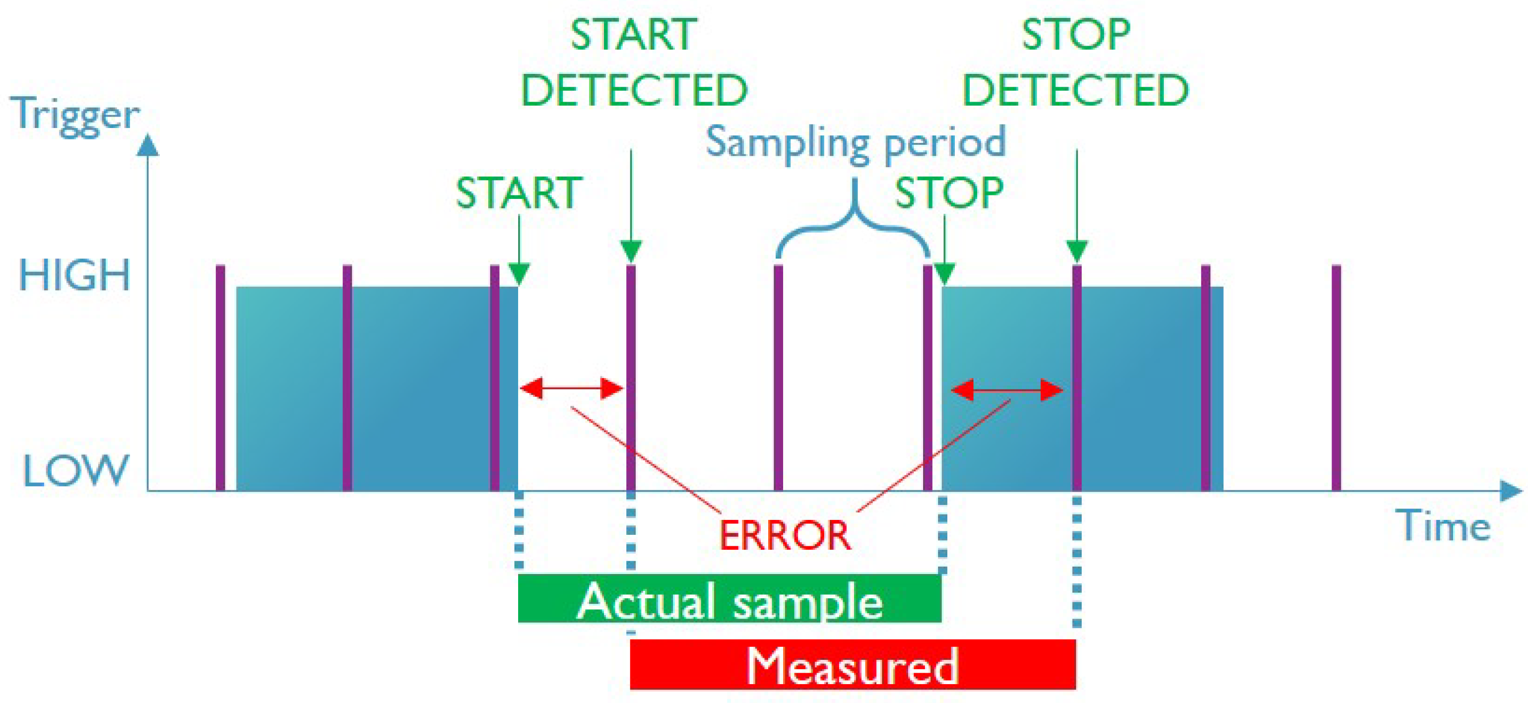
When a new run of the block is initiated, the trigger signal will go high as illustrated in Figure 6. This signal stays high for at least two times the sampling period of the Joulescope, indicated by the vertical lines on the graph. This assures that each trigger signal is captured by the analyser. The actual measurement starts when a falling edge of the first trigger is detected and stops on the rising edge of the next observed trigger signal. The measured samples between these two points are used in the discreet integral to calculate the energy consumption of the executed task. This technique allows us to create tight measurement windows capturing the consumption during the execution of the code of interest. Notwithstanding, the Joulescope’s high sampling frequency of 2 MHz is still relatively low compared to the higher clock frequency of the Nordic nRF52 processor running at 64 MHz. As a result, a sampling error is introduced as highlighted in Figure 6. This error is caused by excluding and including energy buckets that respectively are and are not part of the code execution. For example, the falling edge of the code execution starts at $t_0$ after the last sample was taken. At the next sample point at $t_1$, the energy consumption of the time interval $[t_0;t_1]$ has not been included in the measurement. The opposite situation occurs at the ending side of the measurement. The rising edge of the stop trigger takes place at $t_3$ before it gets sampled at $t_4$. The interval $[t_3;t_4]$ will therefore be included in the energy consumption of the hybrid block while it is not a part of it. In the worst-case scenario, the Nordic board with a clock frequency 32 times higher than the sampling frequency of the Joulescope will have a mismatched window of around $1\mathsf{\mu }$s or 64 clock cycles on the target device.

In order to minimise the impact of the error on the measurements, we apply two strategies. Firstly, the upper bound of the WCEC should always be higher than the actual worst-case to avoid underestimation. Therefore, we propose to include the measured sample before the detected trigger sample. This will introduce additional pessimism to the upper bound, but this overestimation will be less detrimental for the WCEC prediction.

Secondly, the length of the sampling error is independent of the task length. The longer a task runs on the hardware, the smaller the impact of the error will become on the result. For that reason, we have implemented a feature in the COBRA framework that helps expanding the code of a hybrid block when the execution time is too short for sound analysis with the testbench. The Profiling Generator will repeat the code in the block multiple times within one measurement to increase the sample’s execution time. There are two strategies available: loop-based iterations or unrolled iterations. The looped-based iterations will wrap the code inside a loop statement. The unrolled iteration approach will duplicate the code section multiple times equal to the iteration count. This last strategy is not just copying the code X number of times as it will not result in valid code by default, due to possible duplicate declaration exceptions. For the experiments, we used the loop-based iterations for stable performance as the unrolled iteration strategy is still in development. Nevertheless, the COBRA-HPA toolchain takes the usage of looped hybrid blocks into account during analysis. The Feature Generator, for example, will multiply all block features by the number of iterations of the loop and add the overhead of the iteration statement itself to the total.

The acquisition and processing of the sample data is performed by the host computer of the Joulescope. Each sample point, that contains the voltage and current in 13-bit precision and I/O input states [49], is transmitted via USB to the computer at 2 MHz, or 2 million samples per second. At full speed, we will need around 1.5 GB of Random-Access Memory (RAM) to store 60 s of samples. If the computer is unable to process the sample data in time from the Joulescope, then those samples will be dropped by the analyser and lost forever. To handle all these samples in time without requiring a powerful computing system with lots of RAM, we have implemented a moving window on a circular buffer in our testbench drivers. The circular buffer provides a more efficient and stable use of the RAM memory. New samples are added at the end of the buffer while a moving window is accumulating the samples to calculate the energy consumption. The measurement results are written to a log file and reported back to the Profiling Assistant to create the labelled WCEC upper bound datapoints.

3.4.4. Power Supply

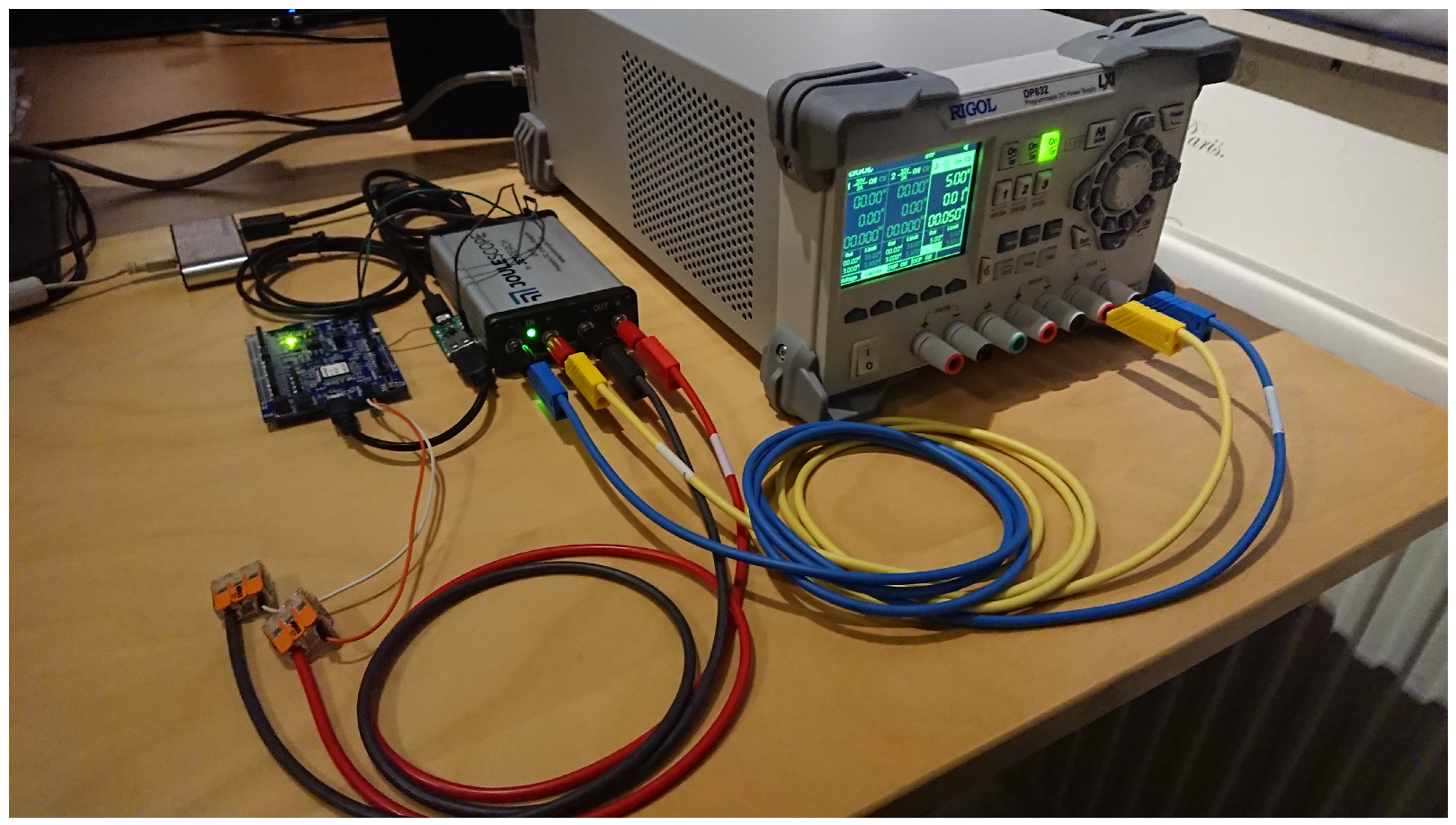
The power supply used in our setup is the RIGOL DP832 programmable DC supply. It has three precision output channels of 3 A each and voltages up to 30 V for a total of 195 W [50]. The Nordic nRF52 operates on a voltage level between 1.7 V and 3.6 V within the limits of the DP832 supply. The result of the final setup with the Nordic nRF52 development board is shown in Figure 7.

4. Results

For this experiment, the eight different regression models of Table 3 are trained with a set of datapoints generated from benchmark code of TACLeBench [41]. A total of 120 small hybrid blocks are generated with the Block Generator from the benchmarks in

Table 5. Benchmarks from the TACLeBench used to generate datapoints for training and validation.

Testbench	Number of Blocks	Lines of Code
Binary Search	12	67
Bitonic	13	72
BSort	15	60
Complex Updates	6	62
Filter Bank	10	89
Insert Sort	15	69
LMS	19	96
Recursion	8	36
ST	22	127

. Each of these benchmarks are split with no abstraction enabled. This results in the generation of default basic blocks. Such basic blocks will contain a single trace of instruction that has exactly one entry and one exit point in its code flow. All generated blocks are then used as datapoints in a 4-fold cross-validation process. Specifically, the datapoints are randomly split to create four sets with 90 elements for training and the remaining 30 blocks as validation.

Each datapoint contains the feature list of all software attributes from Table 2 and the corresponding labelled upper bound measurement from the automated testbench. The aim of this experiment is to evaluate the ability of regression models to approximate the measured upper bound from the testbench, as we want to assess the feasibility of replacing the physical measurements with prediction models. Therefore, we did not evaluate the measured upper bound or the pessimism introduced by the testbench in this paper.

In order to evaluate the performance of our models, we calculated the Mean Absolute Percentage Error (MAPE) on the validation sets. This error metric takes an average of the absolute percentage errors without regard of the sign and is commonly used in forecasts [51] (e.g., regression problems) and other research using prediction models [52], as it is very intuitive to interpret the relative error. The MAPE metric is defined as Equation (1) with h the prediction function (i.e., hypothesis), X the input set of features, m the size of the input set (i.e., number of datapoints) and y the set of actual values or corresponding labels of each datapoint.

$$MAPE(\mathbf{X},h)=\frac{100}{m}\sum _{i=1}^m\left|\frac{y^{\left(i\right)}-h\left({\mathbf{X}}^{\left(i\right)}\right)}{y^{\left(i\right)}}\right|[\%]$$

(1)

During the initial training run, we noticed poor performance of several regression models, among which are the Forest, Random Forest and Support Vector Regressions. After close inspection, we notice that the prediction values of these models converge to one and the same value. Our hypothesis is that an issue occurs with the training of the loss function of the models, due to the extremely small order of magnitude of the provided prediction labels. The energy measurements are expressed in the SI-unit (International System of Units) of energy, the Joule [J]. These values are very small for low-power devices. The dataset we captured from the Nordic board contains on average measurements with an order of magnitude of 10${}^{-6}$ J. To solve this issue, we scaled the labels by shifting the order with the power of 10${}^{10}$ to have enough significant digits before the decimal point. After the scaling, we noticed a significant improvement of the worse performing regression models. In order to further improve the performance of the machine learning models, we need to optimise the training process, the data pre-processing and the model by tweaking the ’settings’ or hyperparameters of the entire processing pipeline. The field of creating these optimised pipelines based on the training data in an automatic manner is called Automated Machine Learning (AutoML) [53]. One of the first AutoML methods was the Tree-Based Pipeline Optimization Tool (TPOT) by the Computational Genetics Laboratory of the University of Pennsylvania [54]. This software package allows data scientist to automate the process of creating a machine learning pipeline, i.e., pre-processing of data, selection of regression models and hyperparameter tuning, that is optimised for a given dataset. For this experiment, we did not implement any AutoML methods yet, but made a first comparison between regression models to study the potential of our methodology while keeping the initial complexity low.

The training of these models requires a decent amount of computation time to complete as this depends on the size of the training dataset, the model complexity and the number of epochs or generations are used for the optimisation of the model and its hyperparameters. The actual evaluation of a datapoint with a trained model only takes a fraction of a second. During our experiments, the training and validation for all models took around 10 min to complete on a laptop with an Intel i7-6700HQ CPU processor. While the training and evaluation require considerable computational power, its resource requirements are less important compared to the prediction performance as the profiling process is carried out offline on the developers computer, and not at runtime. The results of these trained models are listed in

Table 6. 4-Fold cross validated Mean Absolute Percentage Error (MAPE) on the validation set for each trained regression model with relative computation time.

Regression Models	MAPE			Relative Computation Time
	Best	Average	Worst	Training	Predicting
Linear	116%	418.9%	1021.7%	1.73	1
Polynomial (3rd Degree)	8.8 × 10${}^5$%	2.3 × 10${}^9$%	7.7 × 10${}^9$%	20.6	10.3
Decision Tree	6.5%	206.4%	551.1%	1.35	1.46
Random Forest	62.7%	224%	608.1%	25.5	2.73
Support Vector (Linear)	73.4%	190.4%	438.1%	6662.5	2.48
Support Vector (RBF)	71.3%	440.8%	876.3%	2454.4	9.27
K-Nearest Neighbours	42.3%	262.1%	769.9%	1	2.46
Ridge	116%	418.9%	1021.7%	3.21	2.83

. For each model, we show the average and worst-case errors on the validation sets. The last row indicates the relative computation time of each model for training and predicting. A computation time of ’1’ indicates the shortest average execution time of the indicated action between all listed models. The training time for one cross-validation iteration of the K-Nearest Neighbours Regression was the shortest of all models with an average of $1.3$ ms. The Linear Regression had the fastest average prediction time of around 1 ms.

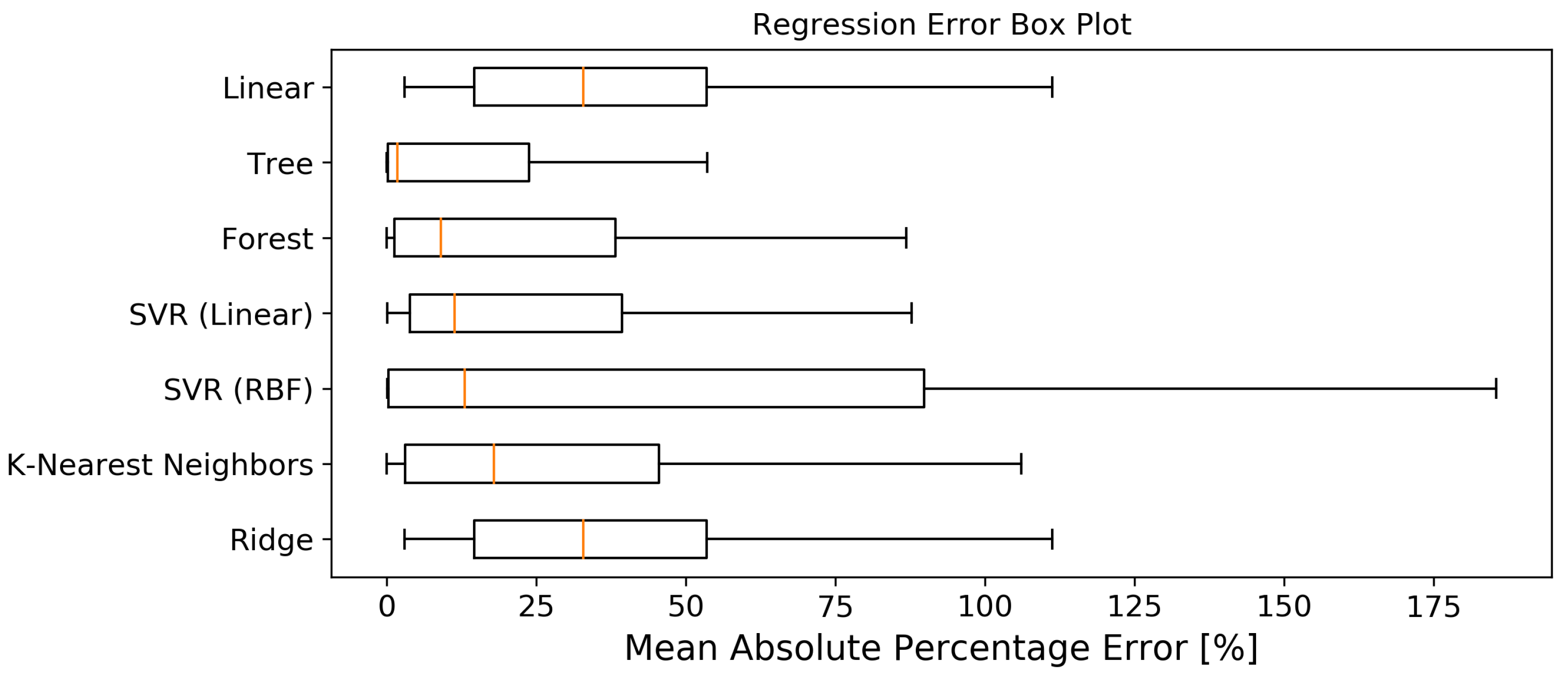
The best performing models in this experiment are on first sight: Decision Tree, Random Forest and Support Vector Regression with Linear Kernel. High deviations are noticeable between the best and worst MAPEs of the cross validated sets. In Figure 8, we plotted a normalised box plot of the error distribution. The polynomial regression was omitted to improve the clarity of the figure.

The graphs in Figure 9 plot the predicted upper bounds for the energy consumption with respect to the actual measured results. The vertical distance between each point and the dotted line in the graph indicates the absolute prediction error for a given datapoint.

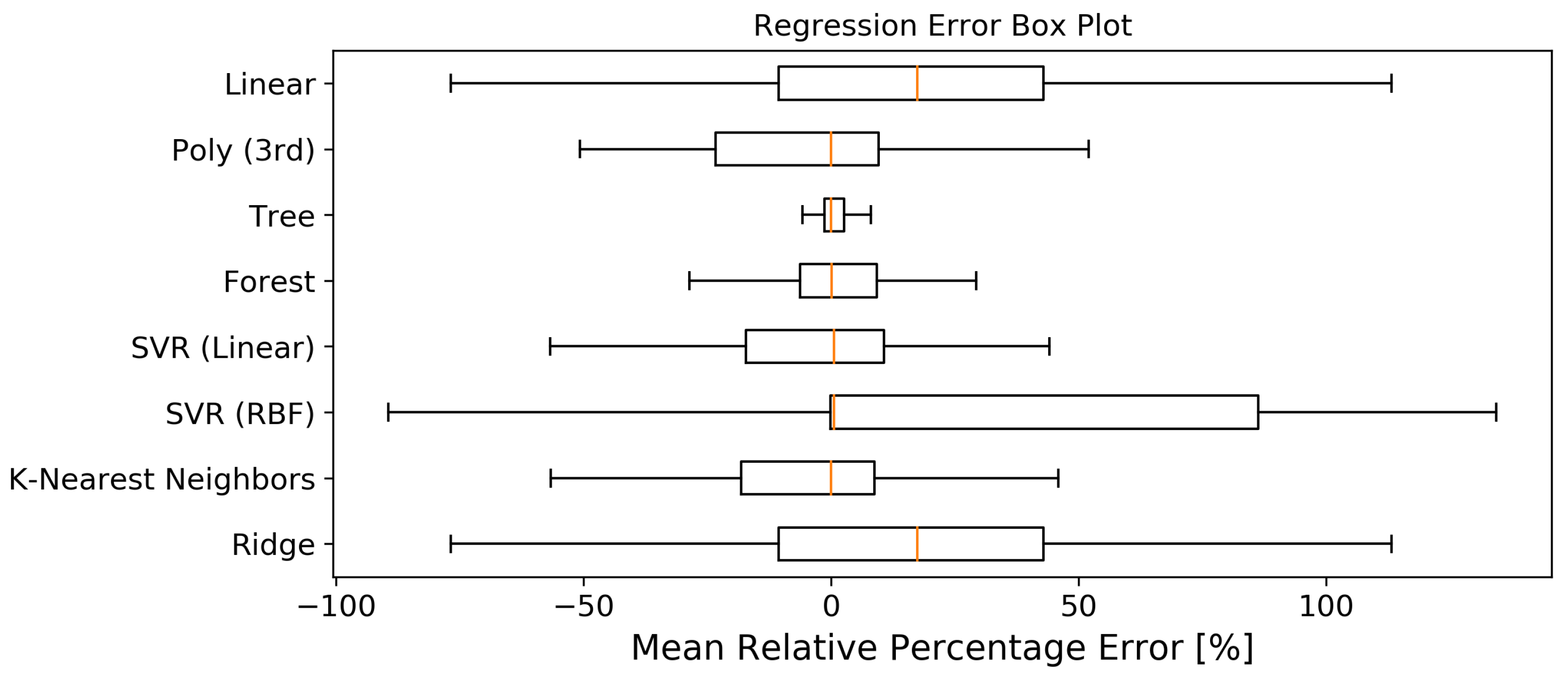
MAPE is an excellent metric to gain insight in the performance of the prediction models. However, there is no indication if the models are mostly over- or underestimating the WCEC. As previous discussed, it is important to keep the upper bound above the real worst-case to avoid compromising the functional behaviour of the system. Therefore, we calculated a Mean Relative Percentage Error (MRPE) for each model in Figure 10. MRPE calculates the percentage difference between the predicted and actual values, but keeps the sign of the error.

5. Discussion

With the automated testbench for the COBRA framework, we were able to generate hybrid blocks from benchmark code and measure the energy consumption on the physical device for upper bound WCEC analysis. A full profiling cycle by the COBRA framework only takes a few minutes depending on the complexity of the program, which most of the time is spent during the actual measurement phase on the Target Hardware. Although this process already automates lots of tedious and time-consuming tasks, it still required manual effort to validate the system operation, such as input set generation and coverage, feature generation, testbench generation and measurement. As a result, the dataset for this experiment is rather small. Nevertheless, we were able to train a set of regression models based on software-related features.

The results of Table 6 show an average percentage error of around 200% for the best performing regression models. These results are already impressive given that they were obtained from the default configuration of the regression models without tuning any hyperparameters in the process, with the exception of the Polynomial and Support Vector Regression with a Radial Basis Function (RBF) kernel. The best models from the list are Decision Tree, Random Forest and Support Vector Regression with a Linear Kernel.

Decision Tree and Random Forest regression are powerful prediction models that make accurate predictions based on the trained data with nonlinear relationships [39]. A decision tree splits the trained datapoints into clusters and assigns a value to them during training, which provides excellent performance on previously seen data. However, the output of the model is discreet. A high partitioning of the tree model is therefore needed to achieve accurate predictions, but this increases the model’s complexity and size tremendously. The model also does not perform well with unseen data during training. The Random Forest, on the other hand, uses an ensemble of randomly generated decision trees whose output is an averaged aggregation from the results of the different decision trees. Therefore, each potentially predictive feature is able to play a role in the decision making instead of being suppressed by others. It is also better in providing predictions of previous unseen datapoints. Nevertheless, both methodologies are very prone to overfitting the training set.

The Support Vector Regression model has on average the smallest MAPE of all models in the experiment. However, these models are very sensitive for differences in the range between input attributes [55]. Providing an upper bound on each attribute, such as number of additions, is not very feasible to determine for different sizes of hybrid blocks. The impact of the scale differences between features was minimal because of the relatively small sized hybrid blocks in this experiment. We could partially tackle this issue by training different models for different split strategies for hybrid blocks and thus, cluster different sizes of blocks.

The worst performing model on the list is the Polynomial regression. On the validation set, the model had extremely high prediction errors compared to the other models. To improve the performance, we applied a grid search to find a better performing lower order degree as polynomial kernel. An optimum was found for a 3rd degree kernel. However, the predictions are still bad. After close analysis, we noticed that the model overfitted the training data excessively with an average MAPE of only 0.75% on the training sets themselves. This overfitting issue is possibly caused by the small size of the training set compared to the number and complexity of attributes used in order for the polynomial model to generalise the problem. The poor performing Polynomial regression can be replaced with Symbolic Regression tools, such as PySR [56] or TuringBot [57], that try to find the best fitting function for a given dataset while preferring the shortest expression [58]. This approach will generate ’simple’ models with better generalisation capabilities, minimising the chances of overfitting the training data due to complex functions.

When we examine the scatter plots of the validation sets in Figure 9, we notice smaller errors in the range of 5000 × 10${}^{-10}$ J and 7500 × 10${}^{-10}$ J where many datapoints are clustered. Datapoints for the higher range are more scarce in the training set, resulting in worse performance. Furthermore, these outliers have an impact on the average error of the models. In order to better compare the performance of the regression models, we have normalised the error distribution and plotted it in a box plot as shown in Figure 8. If we compare the MAPEs of the regression models, we see that the Decision Tree model performs the best with the third quartile ($Q_3$), or 75% of the predictions without outliers, below an absolute error of 23.8% and a median of 1.8%. This model is followed by Random Forest ($Q_3$: 38.2%, Med: 9%) and Support Vector Regression with Linear Kernel ($Q_3$: 39.3%, Med: 11.4%).

An upper bound prediction should try to approximate the real WCEC as close as possible to minimise pessimism. Nonetheless, it should never underestimate the actual WCEC as this could result in detrimental behaviour of the system, e.g., shutdown of the device because of insufficient available energy in the capacitor. In Figure 10, we have calculated the relative error to look at the distribution of under- and overestimated predictions. We note that all regression models are prone to underestimation with their median close to the boundary. Nevertheless, we are able to create an error model based on the validation errors to introduce pessimism to the predictions. This will add a margin to acquire safe upper bound estimates.

The acquired predictions from the WCRC Estimator provide an upper bound of the energy consumption for each given hybrid block. The last step is to combine the predictions of the individual hybrid blocks according to the CFG of the task to obtain an upper bound of the total task. This is achieved with the Analysis Wizard with the use of IPET as discussed in Section 3.3. The list of upper bound prediction per task is exported in a configuration file for the developer.

With the creation of the automated testbench and its integration with the COBRA Framework, we have established the tools and foundation to apply (early stage) WCEC analysis on energy constrained devices, such as batteryless IoT devices. The final process to acquire an upper bound WCEC estimation for the batteryless IoT sensor device we use in the experimental setup (Section 3.1) is as follows. Firstly, we split the software task in smaller hybrid blocks using the COBRA Framework. Therefore, we create a project configuration that describes the block splitting strategy and describes the Target Hardware properties. The tool will generate a list of software features for each hybrid block. Secondly, the user selects an estimator model to perform the prediction for the given Target Hardware platform by providing the software features set. Thirdly, the upper bound predictions are then statically combined and exported for each task by the framework to a formatted text file. Finally, the developer uses the upper bound WCEC estimates from the text file to configure the energy-aware scheduler. The scheduler that is being developed in our experimental setup uses a JavaScript Object Notation (JSON)-formatted file that is read during the boot sequence of the IoT device. If code changes are made to a task, the toolchain needs to profile that task again. The complete toolchain is executed offline when a trained WCRC estimator is used. Therefore, the code profiling process can be executed in the background when the code is developed.

In this paper, we were able to achieve our main goal to create an automated testbench to perform automated energy measurements; and establish a framework to start experimenting with a novel hybrid methodology for WCEC analysis. Our automated testbench and initial work on hybrid machine learning-based WCEC predictions show promising results. However, validation of the hybrid methodology needs to be conducted in future research after improvements to the prediction models are made. The following list provides a summary of action points for future research:

• Feature Engineering: The selection of the right features is an essential part in creating high performing machine learning models. On the one hand, we need to include all features that have a significant impact on the energy consumption of a hybrid block. On the other hand, selecting too many features with less or no relevance will eventually lead to poor performance. This process is also referred to as feature engineering [39]. In order to acquire a set of qualitative features, we need to gain insight in the actual data while looking for correlations between them [37,38].
  As discussed by other researchers in Section 2.3, the energy consumption of the processor is influenced by the data itself due to the flipping of bits. The current attributes used in our experiment do not take any data related features into account except of their scope. Attempts should be made to include more data related features to the attribute list, such as data/array types and sizes, etc.;
• Tuning Predictions Models and Pipeline: Each machine learning model is defined by a set of parameters configuring the training process and the model itself. These adjustable parameters are called hyperparameters [39], e.g., number of hidden layers, learning rate, error penalty, etc. The tuning of hyperparameters is a computational expensive and timing consuming process as the model needs to be trained and re-evaluated over and over again until an optimal MRPE is reached. In practise, hyperparameter tuning can be achieved by a grid search, where each combination of hyperparameters is cross validated to find the best set [39]; or more efficient stochastic search algorithms that explore the state space of the hyperparameters by introducing randomness or noise to the search, such as the TPOT algorithm [54]. For example, the Support Vector Regression with an RBF kernel in the experiment has been tuned with a grid search. The default configuration of the hyperparameters, i.e., C: error penalty and $ϵ$: learning rate, had a real poor performance compared to the other models. This tuning process can be further optimised and extended to the entire processing pipeline with the use of automated AutoML methods [53];
• Increase Training Dataset: In addition to well-designed features, we need a large dataset to train any prediction model. The automated testbench is a first step in quickly acquiring more data. Nevertheless, there are still opportunities to increase the accuracy of the upper bound measurements and speed up the profiling process. One of these improvements would be to include static data analysis in the flow graph. This would allow us to find and generate data input that aims at triggering WCEC paths and lowers the need of manual code annotation. Another approach is to increase the size of the dataset by applying augmentation techniques as proposed by [20,59]. In their research, they created a source code generator that produces pseudo-random code based on the requested characteristics, e.g., flow facts, number of variables, type of instructions, etc.
• Neural Networks: Applying (deep) neural networks as prediction models. These models have the potential to learn complex nonlinear behaviour of the system compared to the regression models. However, these will require much more training data to achieve any reasonable results;
• Different Sized Hybrid Block: The hybrid blocks used in this experiment are all small in size with few instructions. With the hybrid analysis method, we want to explore the balance between the static and measurement-based layer by splitting the code in varying sizes. In a next step, we could explore the influence of using larger abstracted hybrid blocks on the prediction models.

6. Conclusions

The WCEC of software tasks is an important metric for energy-aware schedulers on batteryless devices to guarantee efficient operation. Determining the actual WCEC of a task is not a trivial problem to solve. In this paper, we propose a hybrid methodology that uses machine learning-based predictions to predict an upper bound of the WCEC for small sections of the code, called hybrid blocks. These predictions are then statically combined to get a final upper bound estimation of the WCEC.

Firstly, we presented our HPA extension on the COBRA framework which implements the Hybrid WCRC analysis into the framework. Secondly, we discussed our main work on an automated testbench for the COBRA framework that measures and profiles the upper bound energy consumption on a target device. Finally, we compared the performance of eight different regression models with labelled datapoints generated by the COBRA framework. The results of this first experiment show that the Decision Tree Regression model has the most promising performance. These models could potentially be used in our methodology after additional tuning of the input features and the hyperparameters of the regression models to further improve the accuracy of the predictions.

We believe that this methodology is a feasible solution to gain early insight in WCEC predictions. Therefore, we will continue our research to improve the regression models with more energy related attributes, such as data types and sizes, tuning the hyperparameters of the prediction models, improving the automated testbench for faster and more accurate upper bound measurements and examining other machine learning models (e.g., neural networks).