Abstract
In this paper, a strategy for reducing the electromagnetic interferences induced by power lines on metallic pipelines is proposed and numerically investigated. The study considers a set of steel conductors interposed between the power line and the pipeline. Different shapes of conductor cross sections and different magnetic permeabilities are considered, to identify the solution exhibiting the greatest mitigation efficiency for the same amount of material. The investigation is carried out by means of a quasi-3D finite element analysis. Results show that the main mechanism responsible for the mitigation is constituted by the currents induced in the screening conductors by the power line. Hence, a high magnetic permeability can have a detrimental effect since it reduces the skin depth to values below the size of the screening conductor. In this case, a reduction of the screening current and in the mitigation efficiency is observed. Nevertheless, the study shows that the use of strip-shaped screening conductors allows the employment of cheaper magnetic materials without compromising the mitigation efficacy of the screening conductors.
1. Introduction
The problem of protecting metallic pipelines from electromagnetic induction due to nearby power lines or substations has been extensively studied in the last decades [1,2,3,4,5,6]. These kinds of structures are widely employed for tasks such as water, oil, and gas transportation, and suffer from the effects of both DC and AC electromagnetic interference. These can lead to corrosion, damage to the insulation systems, and also electrical shock for workers working in contact with the metallic structure, depending on the levels of the induced voltages and currents [7,8,9]. Hence, given the high costs and large sizes associated with these structures, accurate predictions of the electromagnetic phenomena involving metallic pipelines constitute a fundamental step for the appropriate design of pipeline–power line corridors and mitigation measures for existing configurations [10,11,12,13,14].
Existing numerical methodologies for the analysis of such interference cases include analytical methodologies based on transmission-line theory and the computation of the mutual impedance between earth-return conductors [15,16]. Finite element analysis (FEA) and combinations between FEA and circuital methods and neural networks [17] are employed as well.
The quasi-3D methodology introduced in [18] is based on the evaluation of the physical dependencies existing among the different conductors of a given corridor section using a series of 2D finite element simulations. The obtained physical information can therefore be embedded in an equivalent electrical circuit, to enforce appropriate constraints on the electromagnetic quantities. This allows complementing the physical assumptions made when the 2D FEA is performed. In this way, the developed technique allows the assessment of groundings or imperfect coatings of the considered metallic conductors in a physically consistent way, while retaining the advantages granted by the use of a FEA.
A previous work [19] has shown that the assessment of simple geometries with the quasi-3D methodology leads to results that are fully compatible with those provided by well-established analytical techniques, such as the one described in the CIGRE Guide on the Influence of High-Voltage AC Power Systems on Metallic Pipelines [20]. Nevertheless, the developed numerical methodology also allows an accurate physical description of complex geometries. These can include any number of buried or overhead conductors, as well as soil models where the electrical resistivity is an analytical function of space.
In this work, the developed methodology is employed to study different configurations and physical characteristics of screening conductors—buried in the soil above the pipeline—that can be employed to screen the metallic pipeline from the electromagnetic field produced by nearby power lines. These screening conductors deviate the magnetic field lines produced by high-voltage AC (HVAC) power lines, exerting a shadowing effect on the underlying pipeline.
Previous works by the authors [21,22] have focused on the influence of the screening conductor’s number, position, depth, and electrical resistivity on their screening efficacy towards a buried pipeline. The aim of the present work is to investigate—for a given cross section of the screening conductors—how the produced mitigation effect is affected by two other factors: the perimeter to cross-section ratio and the magnetic permeability of the conductors. For this reason, the depth of the screening conductors, their distance with respect to the pipeline, their disposition, as well as the resistivity of the employed material will be kept constant throughout this work.
In the following sections, after a description of the developed numerical technique, a typical case of a corridor comprising an HVAC power line and a nearby metallic pipeline buried in the soil is considered. Then, after evaluating the induced voltages and currents in the pipeline in absence of mitigation means, a series of parametric simulations are performed simulating the presence of screening conductors with different shapes and magnetic properties, to identify the most effective configuration for the same amount of material.
2. Numerical Methodology
2.1. Mathematical Model
The quasi-3D method described in the previous section is based on the combination of a 2D FEA and circuital analysis. The FEA is applied to a certain number of 2D cross sections of the considered corridor. The latter typically includes an overhead power line, an underground metallic pipeline, and other additional conductors, such as screening conductors. Each 2D cross section includes the geometrical characteristics of the corridor at a given position along the power line, i.e., the distances between the considered conductors, as well as the electric properties of the soil. These, as shown in [18], may include non-uniformities and stratifications. The employed number of cross sections along the pipeline path influences the accuracy of the final solution [23]. In addition, the considered sections are not physically independent from one another. As anticipated, a circuital methodology is employed to enforce the physical interconnection between these sections. That is, for each considered cross section, FEA is used to extract the parameters of an equivalent multiport circuital component, embodying the local physical characteristics of the corridor in terms of voltages and currents. Finally, the multiport components obtained in this way (one for each cross section) are assembled to form an electrical network that describes the entire corridor.
2.2. Finite Element Formulation
As previously stated, the FEA constitutes one of the main tools employed to obtain the results described in this work. The developed finite element solver is based on a quasi-magnetostatic formulation, where the physical contributions of the displacement current to the magnetic field are neglected. Introducing the magnetic vector potential , such that:
the current density can be expressed as:
where is the electric scalar potential and is the electrical conductivity. In the given assumptions, the magnetic vector potential is governed by the diffusion equation:
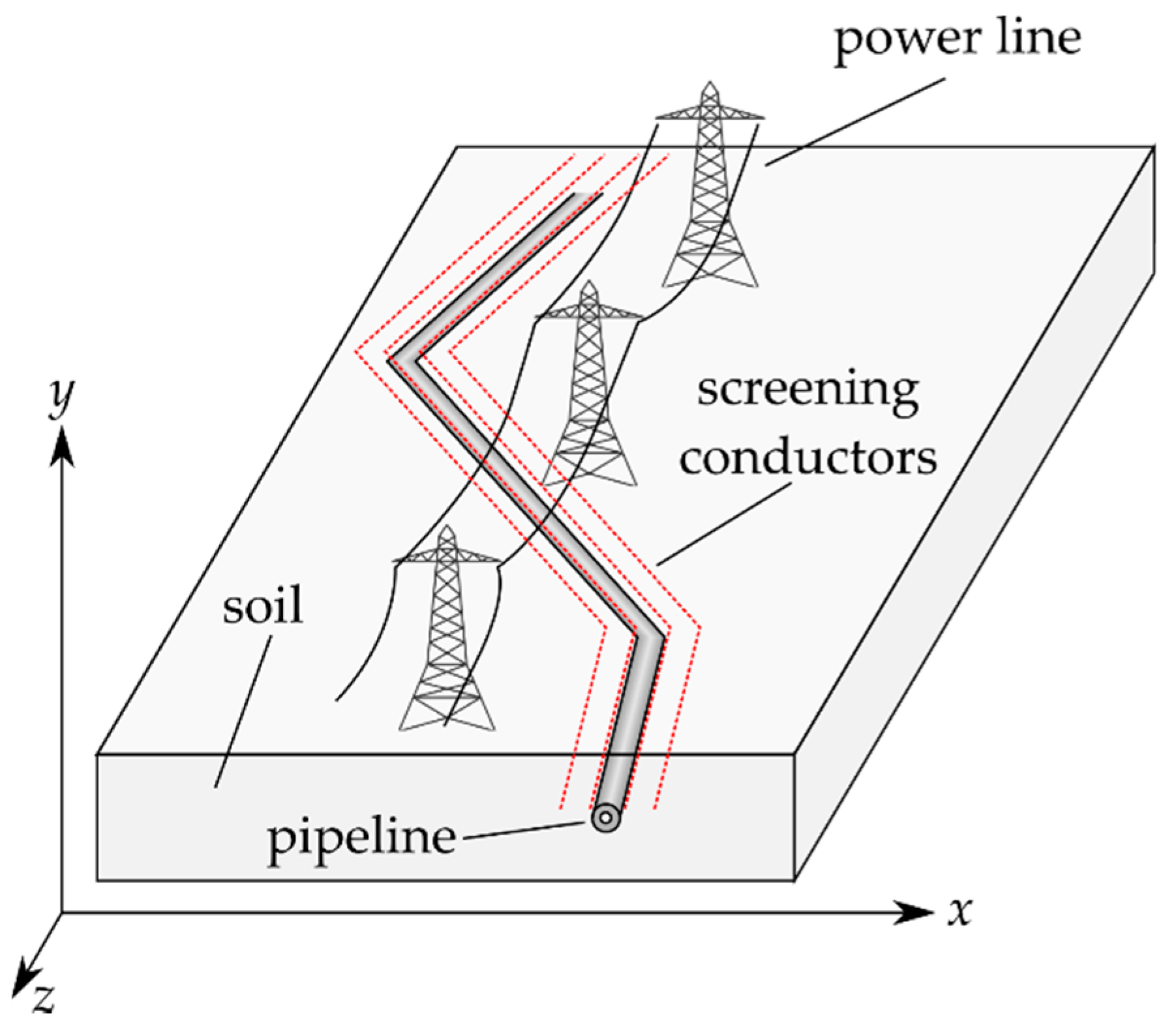
where is the magnetic permeability. The strong preferential direction characterizing the distribution of the current densities in the investigated system allows a 2D approach. That is, in a reference system where the power line is directed along the z-axis of Figure 1, the current density and the vector potential are directed along z as well, and all the electromagnetic quantities are assumed to be independent of z. Hence, , and .

Figure 1.
Sketch of a generic corridor involving an HVAC power line, a metallic pipeline buried in the soil, and several screening conductors, buried in the soil above the pipeline.
In addition, it is assumed here onwards that the magnetic field produced by the power line conductors allows the effects caused by the nonlinear magnetic characteristic of materials having (i.e., magnetic saturation) to be neglected.
The whole system is assumed to operate in sinusoidal steady state, and the materials are considered to be isotropic as well as linear. These assumptions allow us to reformulate Equation (3) with the following stationary complex expression [18]:
In Equation (4), represents the phasor associated with , while accounts for the impressed current densities due to externally applied per-unit-length voltages, i.e., , along the direction. Equation (4) is discretized by means of a finite element method [24]. Considering a given triangular mesh of the calculation domain , the unknown complex function is approximated by a piecewise polynomial function , where and are the arrays containing the shape functions and the nodal values of an array containing the shape functions and values of . A Galerkin approach yields the following linear algebraic system:
The coefficient matrix in Equation (5) is a complex matrix defined as:
where is a matrix formed by the components of the shape functions’ gradient. and the boundary condition enforced on the magnetic vector potential are taken into account in the right-hand side of Equation (5), which is defined as:
Thus, the solution of Equation (5) yields the nodal values of as a response of the forcing terms (i.e., the impressed current densities ). In this respect, Equation (5) represents the dependence of the electromagnetic behavior of a corridor section as a function of the voltage applied in the z direction. Thus, Equation (5) is used to extract the parameters defining an -port circuital component, which embodies the dependencies existing among all the conductors (i.e., power line, OGWs, earth, …) in a given corridor section. In this framework, the employed circuital technique allows the physical interactions between the various sections along the power line to be modeled. The effects of non-longitudinal (i.e., that are not directed along the direction) currents can be taken into account as well, connecting the different conductors with appropriate impedances.
2.3. Equivalent Circuit
A generic routing of the pipeline with respect to a power line (i.e., where the two structures are not necessarily parallel) can be approximated by splitting the pipeline into a sequence of sections. In the generic section, all the conductors are assumed to be parallel to the power line (directed along , so that the aforementioned assumption on the direction of the magnetic vector potential and the current densities (, ) holds for each section. As mentioned before, the FEA is employed to evaluate the current density distribution on the cross section corresponding to each subdivision of the routing. With reference to the schematic representation in Figure 2, the obtained current density in a given cross section of the routing, can be integrated over the generic conductor to obtain the electric current .
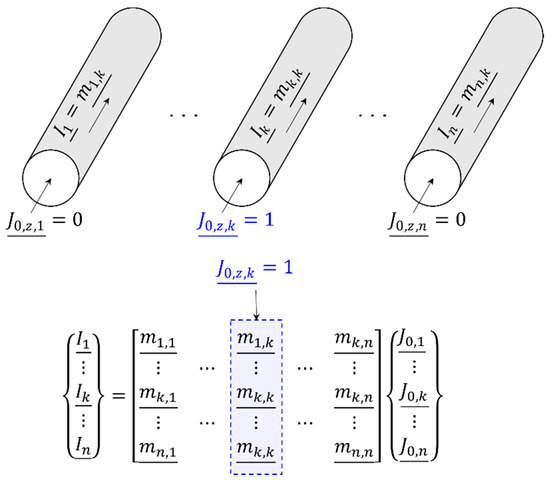
Figure 2.
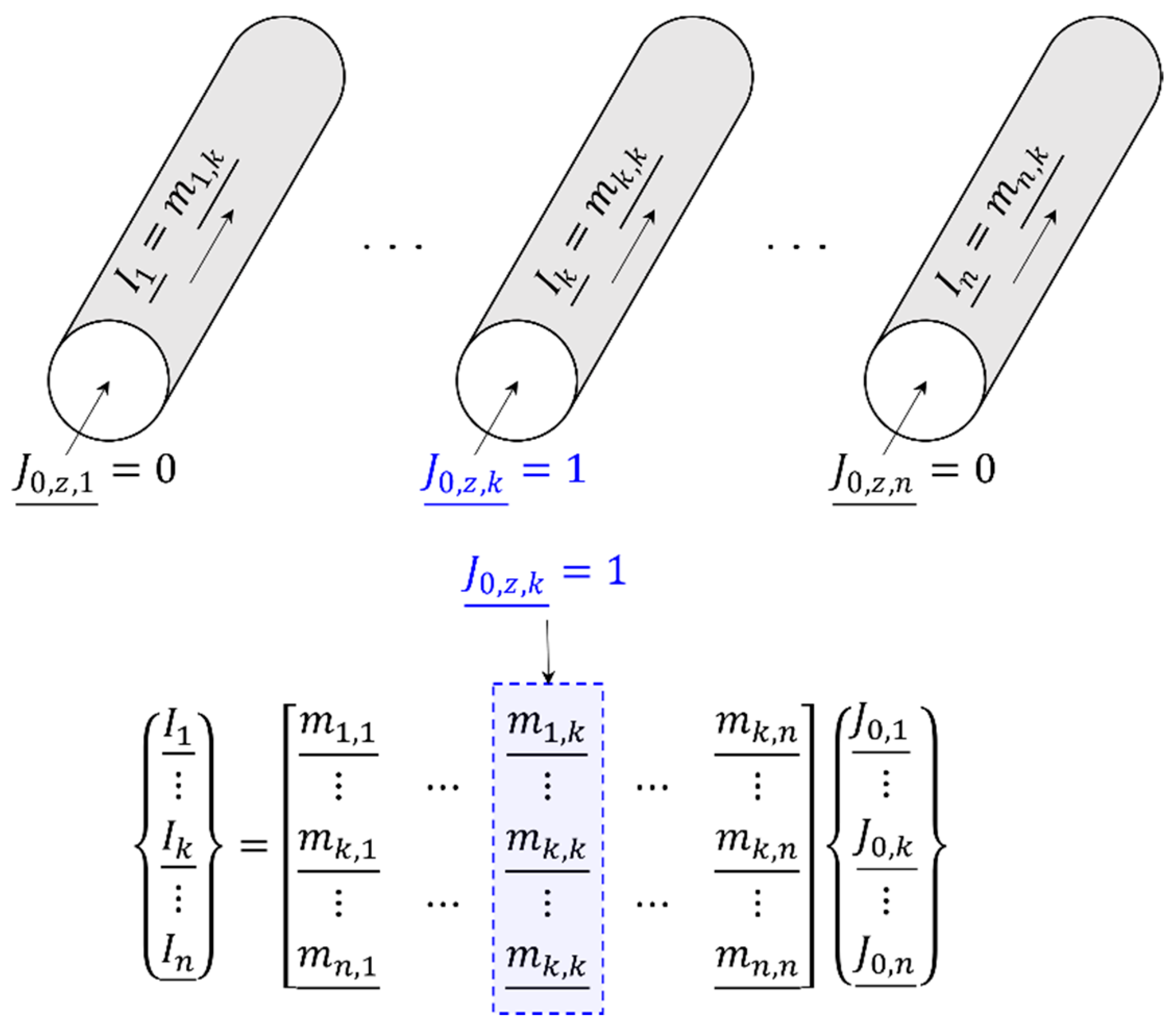
Sketch of the methodology employed to extract the –th column of the characteristic matrix for a given cross section of the geometry, using 2D FEA.
This allows us to obtain a linear relationship linking the array , i.e., the currents crossing the conductors in the considered cross section, and the forcing term array . The entries of are the impressed current densities on the conductors. The derived linear relationship is written as:
The matrix in Equation (8) is defined as the characteristic matrix, and it is the output of the FEA for each considered cross section of the routing. The generic entry of depicted in Figure 2 is the current induced in the –th conductor when a unit current density is enforced on the –th conductor. For the given cross section, the characteristic matrix is computed by running instances of the developed finite element solver. For each run, a unity current density A/m2 is enforced on a different (single) conductor. The values along the –th column of correspond to the obtained currents on the conductors when .
If is the electrical conductivity of the –th conductor, and if is the length in the direction associated with the given section, the forcing term can be expressed as
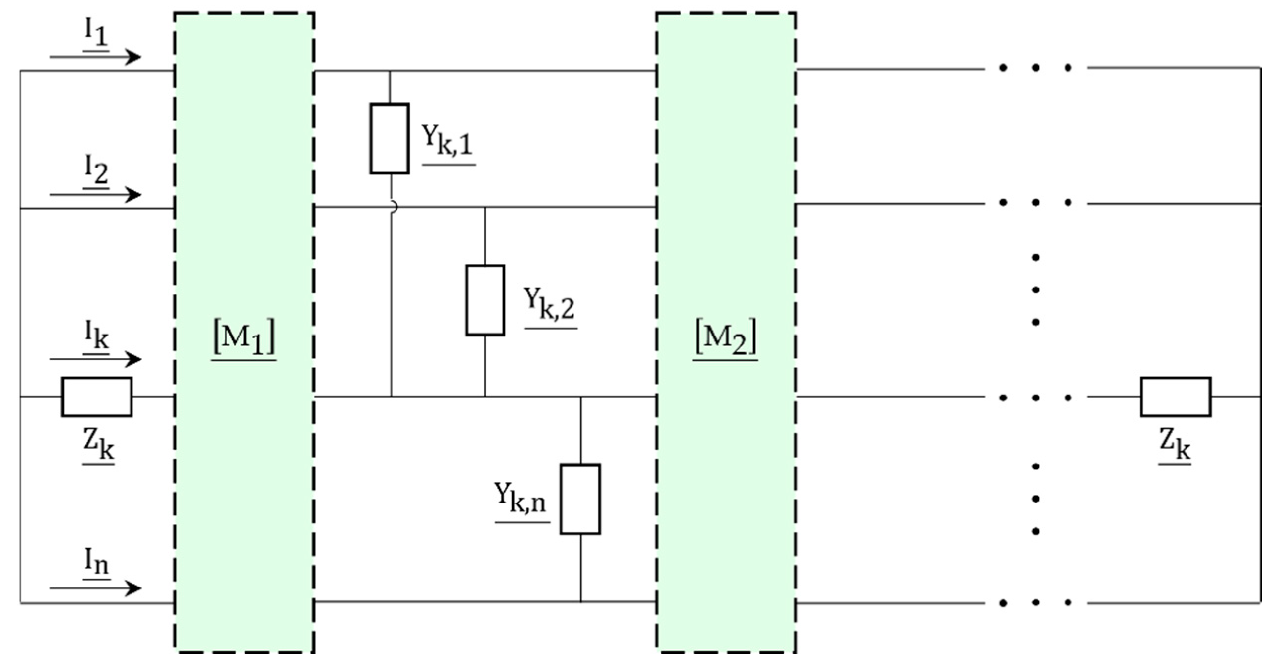
where is the voltage applied to the conductor along its length. Thanks to Equations (8) and (9), the generic characteristic matrix can then be regarded as the constitutive relation of an -port circuital component. Each -port is then inserted into a cell of an equivalent circuit representing the whole corridor. The process is shown, for a general configuration consisting of conductors, in Figure 3. In this way, every cell features several per-unit-length admittances, connecting the earth-return conductors (such as the pipeline or the overhead ground wires, OGWs) to the soil. Finally, the numerical solution of the equivalent circuit is performed by means of the tableau analysis technique, as detailed in [19].
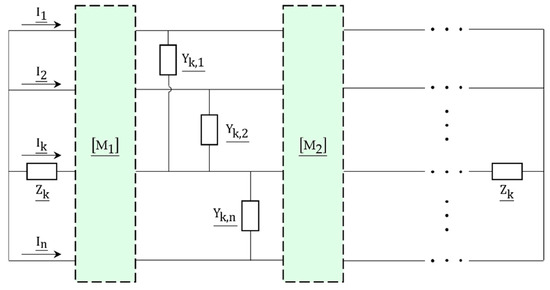
Figure 3.
General topology of an equivalent circuit; each characteristic matrix is extracted by performing 2D FEA on a single cross section of the corridor. For the sake of readability, only the terminal impedances of the –th conductor and the admittances between the –th conductor and the remaining ones have been represented.
3. Simulation of a Nonparallel Pipeline–Power Line Routing
This section is devoted to the numerical simulation of mitigation methodologies that can be employed to reduce voltages and currents induced in pipelines by nearby HVAC power lines. In particular, the methodology described in Section 2 is employed to compare the effectiveness of different shapes and physical characteristics of the employed screening conductors (the term mitigation wires is also commonly employed by other authors and sources). The study is performed by comparing the magnitudes of the pipe-to-soil voltage (i.e., the voltage between a given point of the pipeline and earth) and the pipeline current induced by the HVAC when different shapes and values of relative magnetic permeability of the screening conductors are employed. This section is subdivided into two main parts. The first part is dedicated to the description of the studied configuration; the geometrical and the electrical characteristics of the modeled conductors are discussed from the perspective of their role in the equivalent network, built using the physical information extracted via the FEA. In the second part of the section, the results of the performed parametric simulations are presented and compared to a reference case, where no screening conductors are employed.
3.1. Configuration Description
3.1.1. Pipeline–Power Line Routing
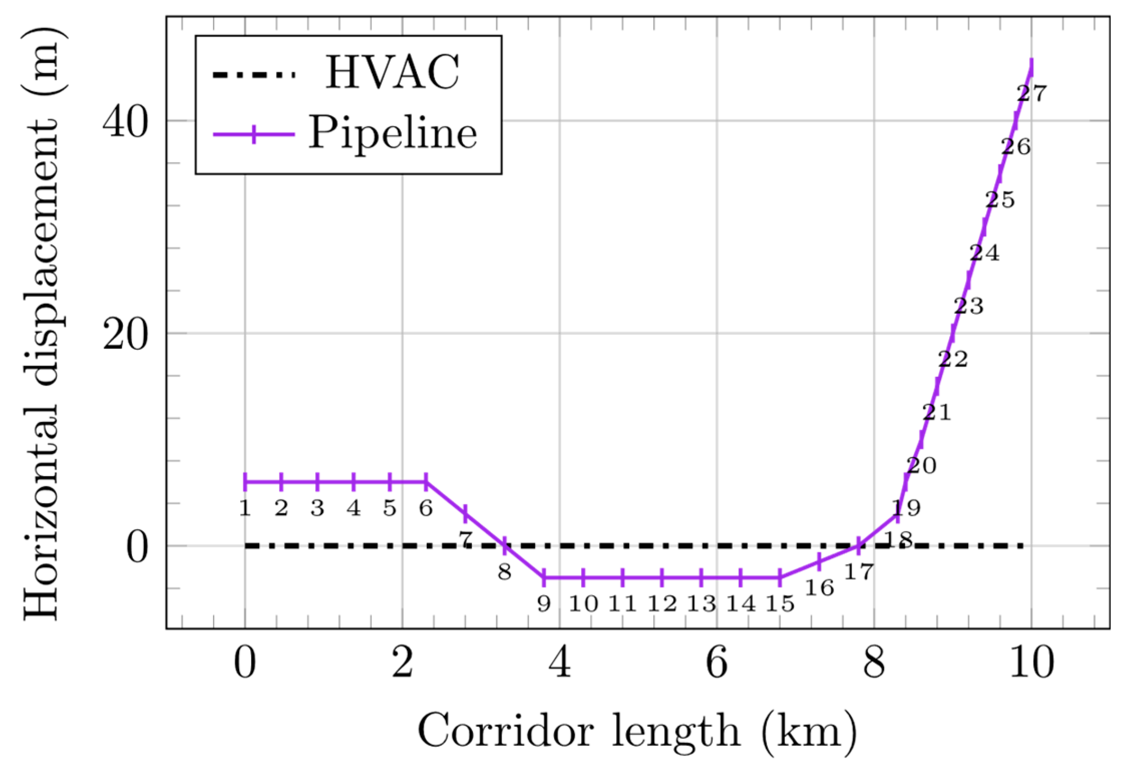
The screening conductors, buried in the soil above the pipeline, follow the pipeline route depicted in Figure 4. In the same picture, the numbers 1 to 27 indicate the different cross sections of the corridor that have been considered in the FEA. The pipeline path crosses the HVAC power line two times, with different crossing angles. This nonparallel configuration represents a more general case with respect to parallelisms. Further details on the discretization of the studied configuration, the numerical implementation of the methodology, and the adopted boundary conditions can be found in Appendix A.

Figure 4.
Pipeline horizontal displacement with respect to the HVAC power line center along the length of the corridor; the screening conductors follow the pipeline path, and are buried in the soil at a constant depth; the numbers from 1 to 27 denote the different 2D cross sections of the geometry used in the FEA.
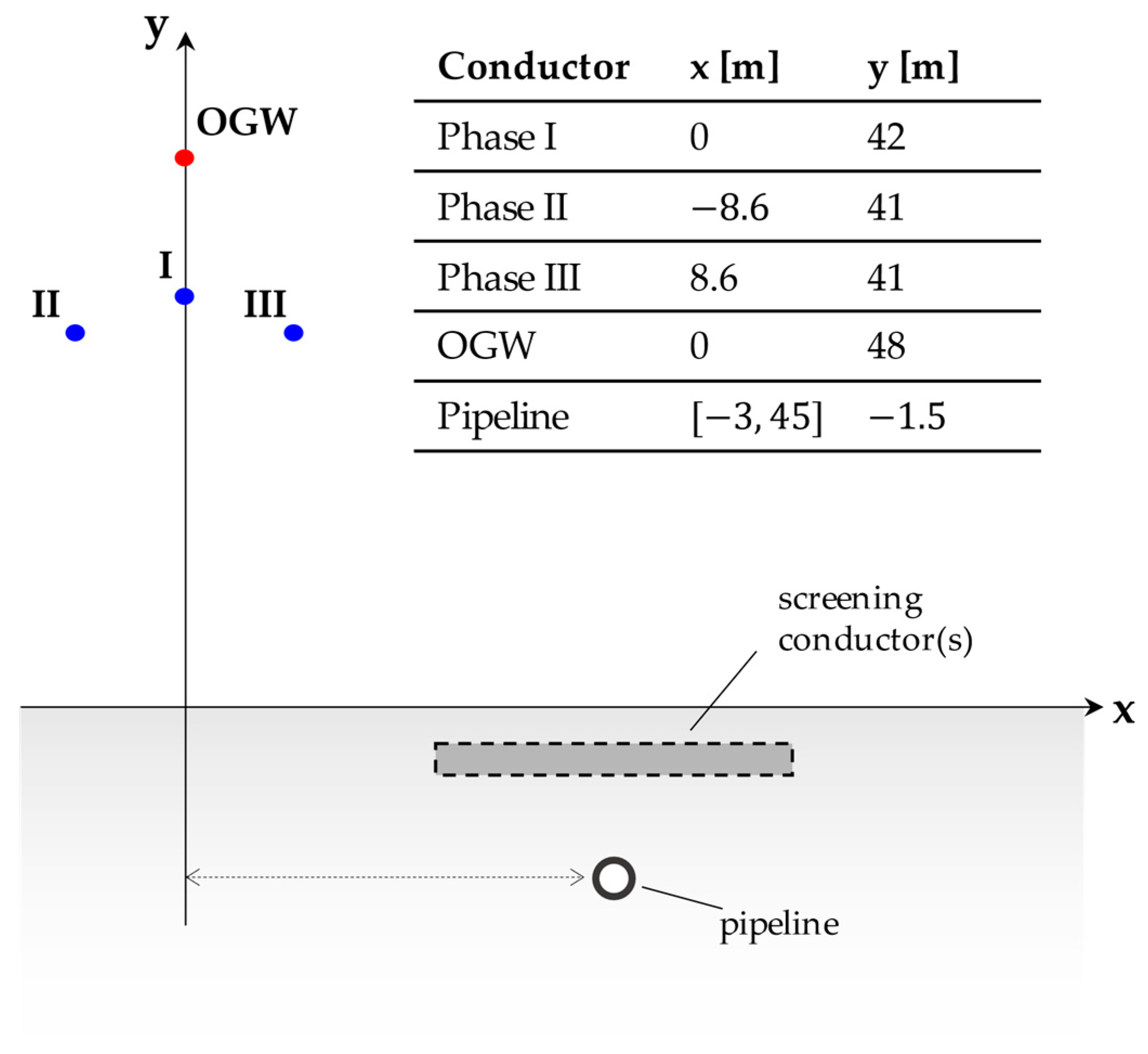
A schematic representation of a generic corridor section is shown in Figure 5. The position of the power line conductors is reported alongside with (constant) pipeline burial depth. As can be observed in Figure 4, the pipeline horizontal displacement with respect to the power line is between −3 m and 45 m, depending on the considered section. This is reported in Figure 5, and it applies to the screening conductors, too. The 27 sections in Figure 4 are obtained by displacing (horizontally) the pipeline and the screening conductors (if present), while the position of the power line conductors is retained throughout all the different sections.
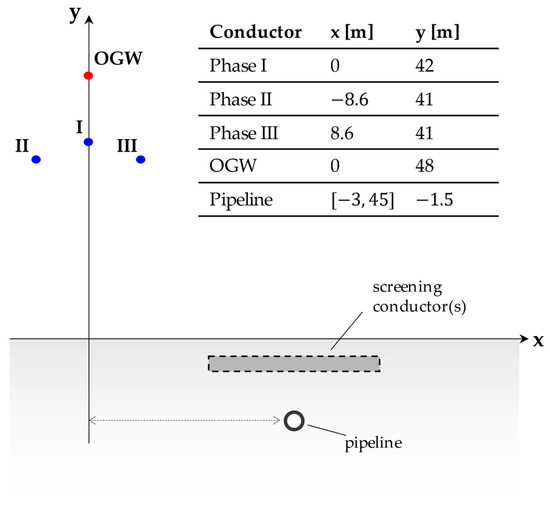
Figure 5.
Generic 2D section of the pipeline–power line corridor; position of the power line conductors and pipeline depth; the interval refers to the pipeline horizontal displacement with respect to the power line center throughout the different sections (see Figure 4) employed to discretize the corridor; details on the shape and positioning of the screening conductors are provided in a dedicated figure.
3.1.2. Screening Conductors
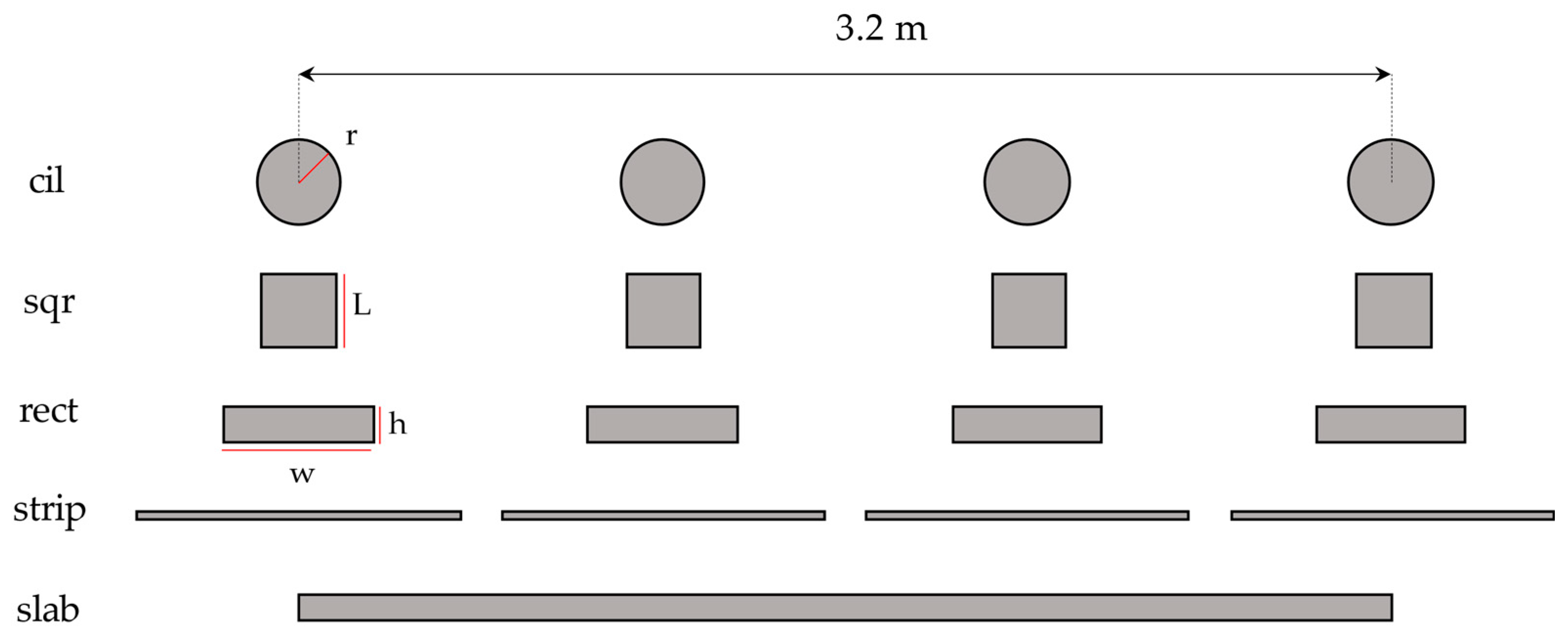
Figure 6 shows the five different shapes and configurations of screening conductors considered in this work. The first configuration (cyl)—also studied in [21,22]—is composed of 4 equispaced cylindrical conductors, with a radius . This shape of the screening conductors has the advantage of being easily accessible, since it is typically employed for reinforcement steel bars in the construction industry. The centers of the four cylindrical conductors are distributed following a horizontal segment of 3.2 m.
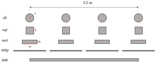
Figure 6.
Screening conductors’ arrangements employed in the study; Configurations strip and slab are not to scale; , , , , , , , and ; the screening conductors follow the same routing as the pipeline, and are buried 0.25 m below the soil surface.
The second configuration is composed of four equispaced square conductors (sqr), with the same cross section of the cylindrical screening conductors. Hence, the edge of these square conductors is . As a consequence, even if the cross section of the sqr conductors is the same as cyl, the perimeter-to-area ratio is higher in this second case.
The third (rect) and the fourth (strip) configurations are obtained by further increasing the perimeter, while keeping the same cross section. In the rect configuration the four conductors are rectangular, with width and height , while for the strip configuration and .
The fifth configuration (slab) features a single screening conductor, with and . The has the same width as the whole 3.2 m segment to which the centers of the conductors belong in the first four configurations. Hence, the slab is characterized by a considerably larger cross section compared to the other described configurations. The cylindrical, square, rectangular and strip screening conductor configurations have been obtained using an equal cross section criterion. Since the same material is considered, this criterion yields an equal weight of the employed material for the aforementioned four configurations. The slab configuration is an exception, since it features a considerably larger cross section. Differently from the other four screening conductor shapes, the idea behind the slab is not to provide a realistic technical solution, but rather showing a limiting case that is used as a reference. In this way, the results yielded by the slab configuration show how close to an ideal case the results obtained with the other configurations are.
3.1.3. Equivalent Circuit, Electrical, and Geometrical Data
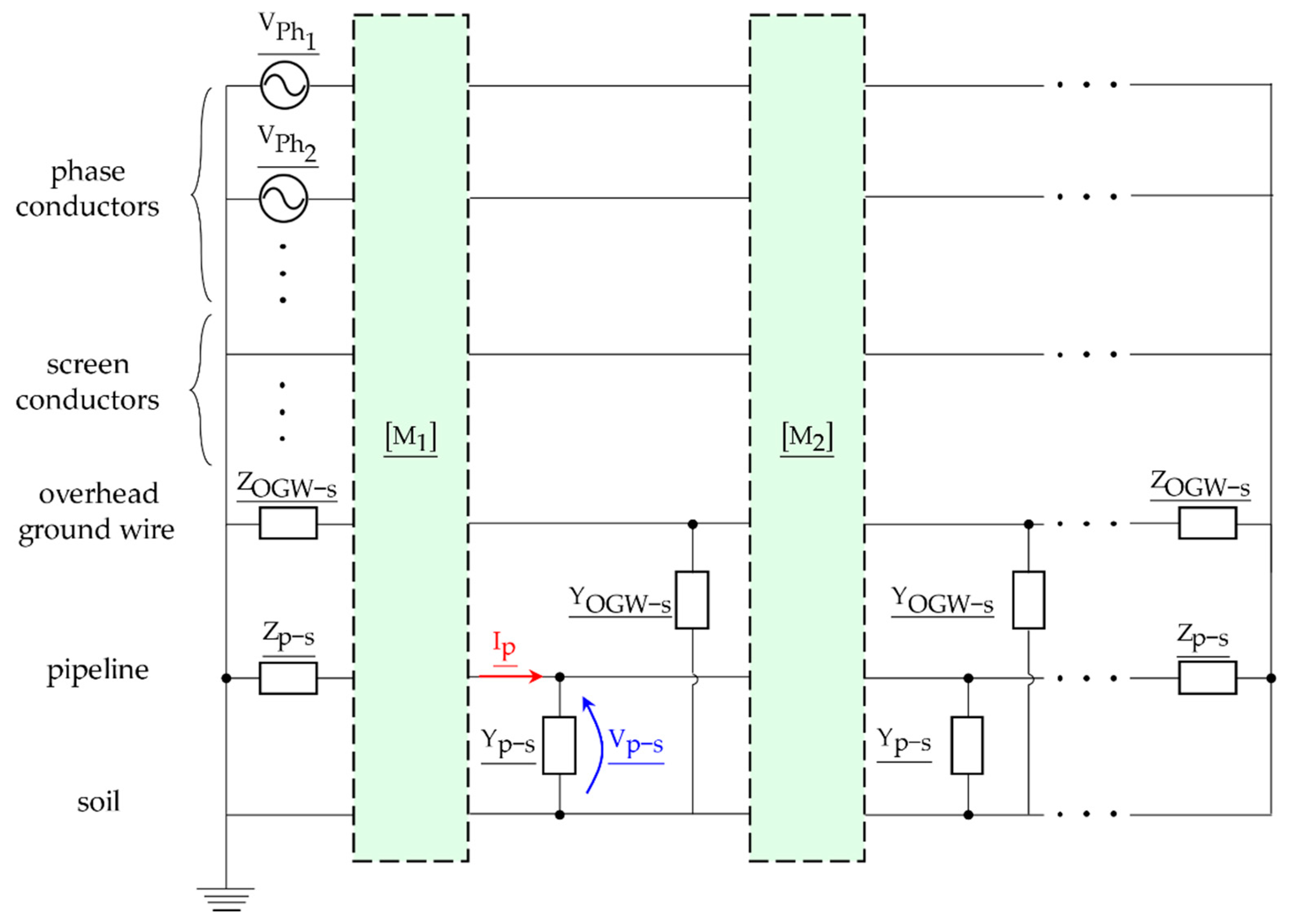
The application of the methodology described in Section 2 to the described pipeline–power line routing leads to the construction of the equivalent network depicted in Figure 7. The figure shows the first two cells of the equivalent network, embodying the corresponding characteristic matrices, extracted via FEA of the first two corridor cross sections indicated in Figure 4. The equivalent network includes the power line conductors, i.e., the three-phase conductors, and an overhead ground wire (OGW). The OGW is connected to the soil at both ends of the domain by means of two equal terminal impedances . The OGW is also connected to each power-tower grounding system, represented by an admittance between the OGW and the soil in each cell of the circuit. The same reasoning is applied to the pipeline. The pipe-to-soil voltage phasor is indicated in blue in the drawing, while the pipeline (longitudinal) current is marked in red. It should be highlighted that , the pipe-to-soil voltage, can also be obtained as the voltage drop due to the (transversal) current flowing through the pipeline coating () at each cell of the circuit. The network in Figure 7 has been employed to obtain all the numerical results that will be presented and discussed in the next sections of this work.
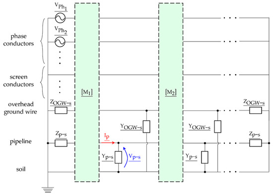
Figure 7.
Pipeline–power line corridor equivalent circuit; each characteristic matrix is extracted by performing 2D FEA on a single cross section of the corridor.
The electrical and geometrical characteristics of the considered physical configuration are reported in Table 1. Unlike the other metallic conductors, for the sake of simplicity, the screening conductors are assumed to be perfectly insulated from the soil within the routing, giving , where is the per-unit-length admittance of the screening conductor to earth. The physical impact of non-negligible admittances to soil on the screening conductor currents will be discussed in a future work.

Table 1.
Geometrical data and material properties adopted in the simulations.
3.2. Simulation Results
3.2.1. Induced Voltage and Current in Absence of Screening Conductors
In order to provide a reference case for the evaluation of different shapes and characteristics of the screening conductors, the configuration described in the previous section is firstly assessed assuming the absence of any mitigation measures. Hence, in this case only the soil exerts a screening effect towards the induced voltage and current on the pipeline. Figure 8a,b show the obtained pipe-to-soil voltage () and longitudinal pipeline current () along the length of the simulated corridor. These results are yielded by the network analysis of the equivalent circuit shown in Figure 7, without the screening conductors. At this point, it is worth highlighting that—even if the term network analysis is used for the sake of conciseness—the tableau analysis is carried out using physical information extracted through FEA of the discretized domain, as described in Section 2. The obtained results show that both the induced voltage-to-soil and current reach considerable values, requiring the employment of mitigation means [27]. As one can see, a dual behavior can be observed in the induced current and voltage profiles, i.e., the zones with large values of correspond to low values of , and vice versa. This can be explained considering that—as anticipated in Section 3.1.3—with reference to Figure 7 can be regarded as the voltage drop due to the (transversal) current flowing through the pipeline coating () at each cell of the circuit.
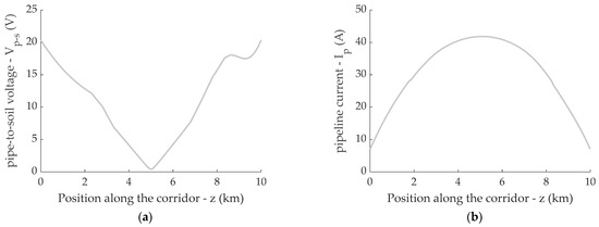
Figure 8.
Induced pipe-to-soil voltage (a) and current (b) along the corridor when no screening conductors are employed (reference for voltage mitigation effectiveness).
3.2.2. Parametric Analysis of Electromagnetic Screening Effectiveness
In the previous section, the routing described in Figure 4 was simulated without any screening conductor. Hence, the results in Figure 8 represent the unmitigated voltage and current induced in the pipeline by the currents flowing through the nearby HVAC power line.
In this section, the same pipeline–power line corridor is simulated adding—in turn—one of the five different sets of screening conductors shown in Figure 6. The set of simulations is then repeated four times, to cover a range of relative magnetic permeability of the steel screening conductors, from 1 to 1500.
3.2.3.
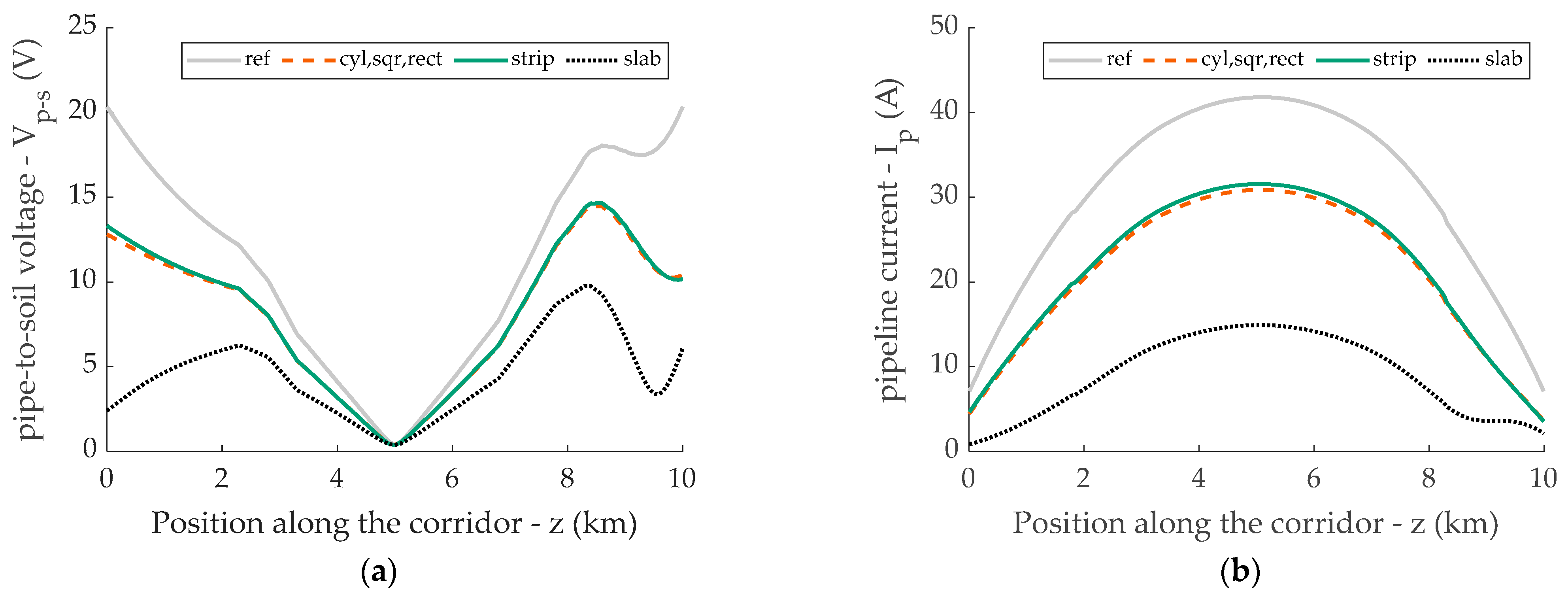
Figure 9 shows the induced voltage-to-soil (a) and current (b), for the five different screening conductor configurations, when the (relative) magnetic permeability of the steel screening conductors is set to unity, . The comparison with the unmitigated results (grey continuous line) shows that a marked reduction of both and is achieved with all the tested configurations. Still, mitigation obtained with the slab configuration is considerably higher than that obtained with the previous configurations.
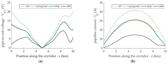
Figure 9.
Induced pipe-to-soil voltage (a) and current (b) along the length of the corridor for different shapes of the screening conductors when the magnetic permeability of the screening conductors is set to 1 (); the results obtained the cyl, sqr, and rect screening conductors have been grouped for the sake of readability; the unmitigated results (grey continuous line) are marked as ref.
This is expected, since the cross section of the slab is larger than the other configurations, leading to a higher induced current on the screening conductor, exerting in turn a more pronounced mitigating effect by screening the pipeline from the power line electromagnetic field.
Focusing on the results obtained using the remaining four configurations (with the same cross section), the induced voltage and current obtained when , sqr, and rect are employed are almost identical, so that a single dashed line has been used to represent the three results for the sake of readability. This can be explained considering that the skin depth at a frequency of for steel ( S/m) is mm. The induced current density for the three configurations can therefore be reasonably considered as uniform. Given that the cross section is the same, an approximately equal current must flow through , sqr, and rect yielding the observed similar mitigating effect.
The same reasoning can be applied to the strip configuration, which is obtained by further increasing the perimeter-to-area ratio with respect to rect. As can be observed, the strip mitigation efficiency for suffers a slight decrease (i.e., higher values of and are obtained) compared to the other cross sections. This result can be explained by observing that the mitigating effect is mainly due to the currents that are induced by the overhead power line in the screening conductors. A strip cross-section conductor is inherently less efficient in producing a magnetic field in the close vicinity of the conductor itself. Indeed, considering a conductor with a circular cross-section A carrying an electric current I, the magnetic field on the outer surface of the conductor can be easily calculated as . Conversely, the magnetic field on the surface of a strip-conductor carrying the same current I, can be estimated neglecting the end effect as where is the strip width. Then, the ratio inversely depends on the width , implying that the wider the strip, the lower is the magnetic field in the region exposed to its wide edge. Of course, this difference becomes negligible for large distances from the screening conductor, but in the proposed study this mechanism apparently plays some kind of physical role.
3.2.4.
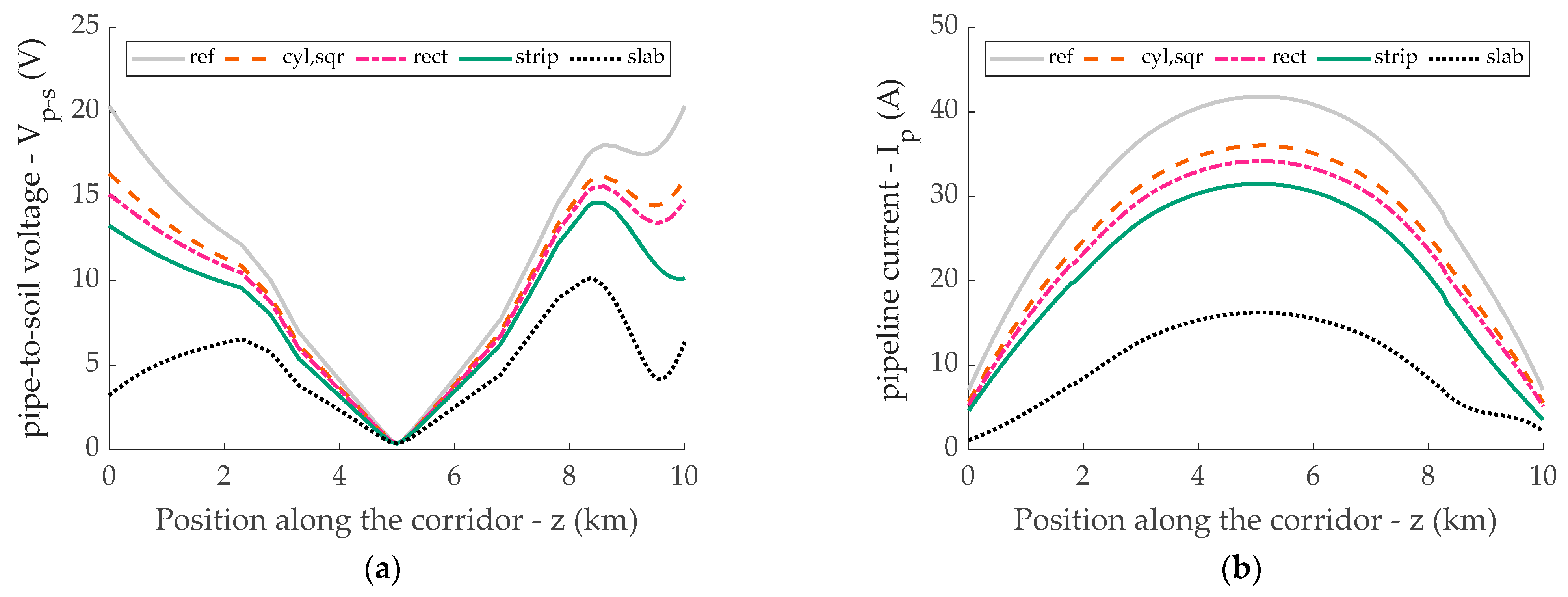
The parametric simulation described in the previous paragraph for is repeated for increasing values of relative magnetic permeability of the screening conductors. In order to obtain the results in Figure 10, Figure 11 and Figure 12, the value of has been set to 250, 500, and 1500, respectively, to assess the influence of this parameter on the screening effectiveness of the conductors. Starting from Figure 10, it can be noticed that—while the results yielded by cyl and sqr are still very close—a noticeable difference can be now appreciated with the rect configuration. In particular, the latter produces a higher screening effect with respect to cyl and sqr. This is due to the skin depth ( mm), well under the characteristic length of cyl () and sqr (). The rect configuration, having a smaller height (), is less affected by the skin effect, leading to slightly higher mitigating effects towards both the induced voltage and current. The same rationale can be applied to the strip, where the perimeter-to-area ratio is further increased with respect to rect , which is lower than the skin depth for the considered electrical conditions, granting a higher level of induced current.
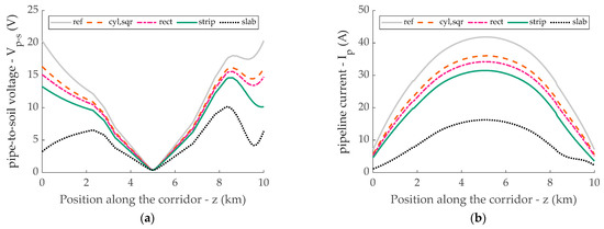
Figure 10.
Induced pipe-to-soil voltage (a) and current (b) along the length of the corridor for different shapes of the screening conductors when the magnetic permeability of the screening conductors is set to 250 (); the unmitigated results (grey continuous line) are marked as ref.
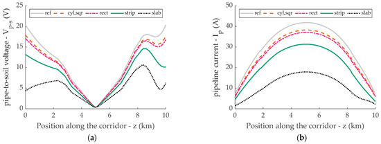
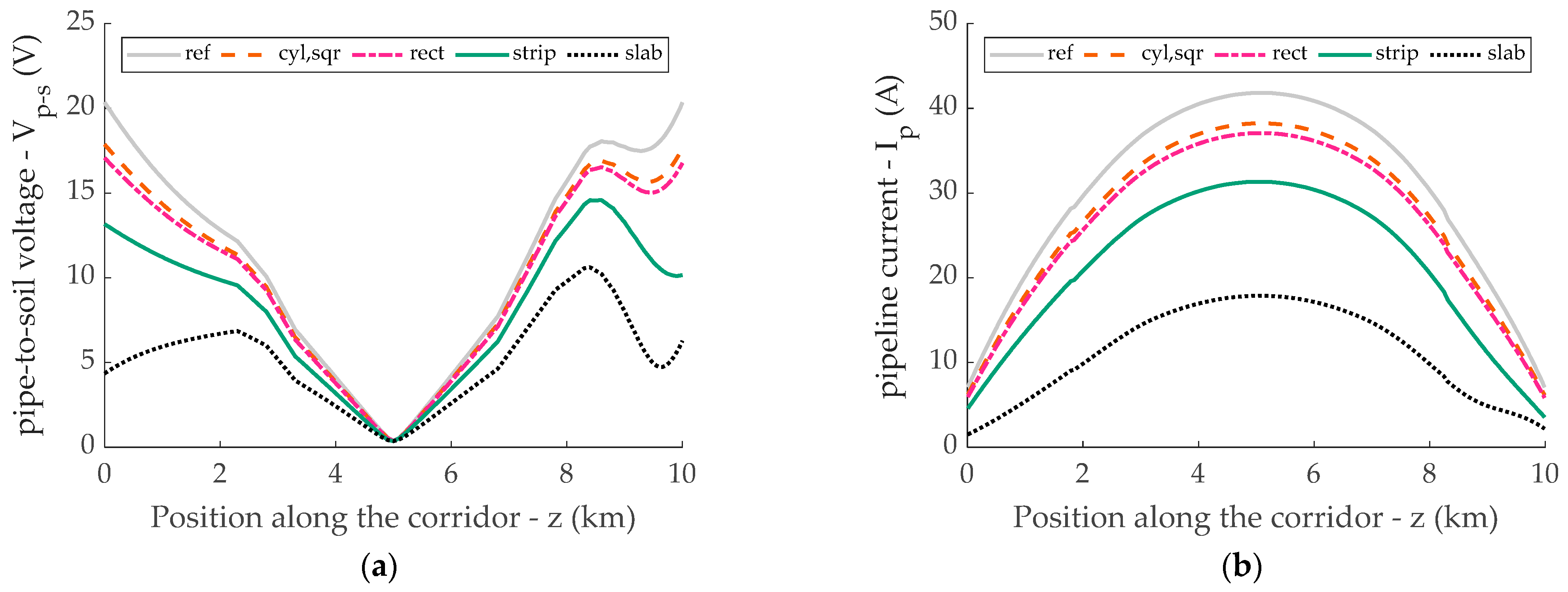
Figure 11.
Induced pipe-to-soil voltage (a) and current (b) along the length of the corridor for different shapes of the screening conductors when the magnetic permeability of the screening conductors is set to 850 (); the unmitigated results (grey continuous line) are marked as ref.
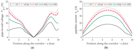
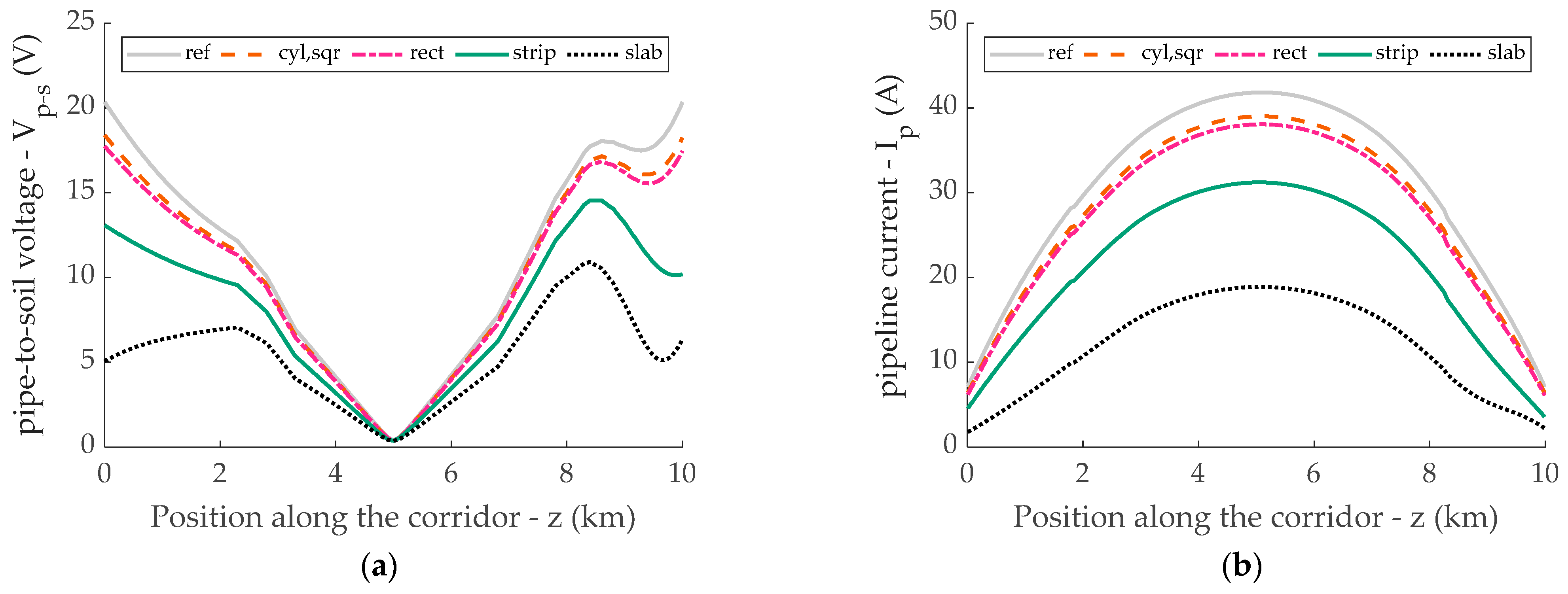
Figure 12.
Induced pipe-to-soil voltage (a) and current (b) along the length of the corridor for different shapes of the screening conductors when the magnetic permeability of the screening conductors is set to 1500 (); the unmitigated results (grey continuous line) are marked as ref.
Comparing Figure 10 to Figure 9 (where , ), a marked difference can be found in the results corresponding to cyl, sqr, and rect. However, the difference between the two plots is more subtle when strip is considered, since in both cases the reduced height of the conductor allows for an approximately uniform current density distribution.
The same trend described for Figure 10 can be noticed in the results depicted in Figure 11 and Figure 12, where the relative magnetic permeability is increased to 850 and 1500, respectively. Consequently, the screening conductor skin depth decreases to and mm, respectively. The comparison between these results and the ones in Figure 9 where show that the cylindrical, squared, and rectangular screening conductors become ineffective for higher values of magnetic permeability.
4. Discussion
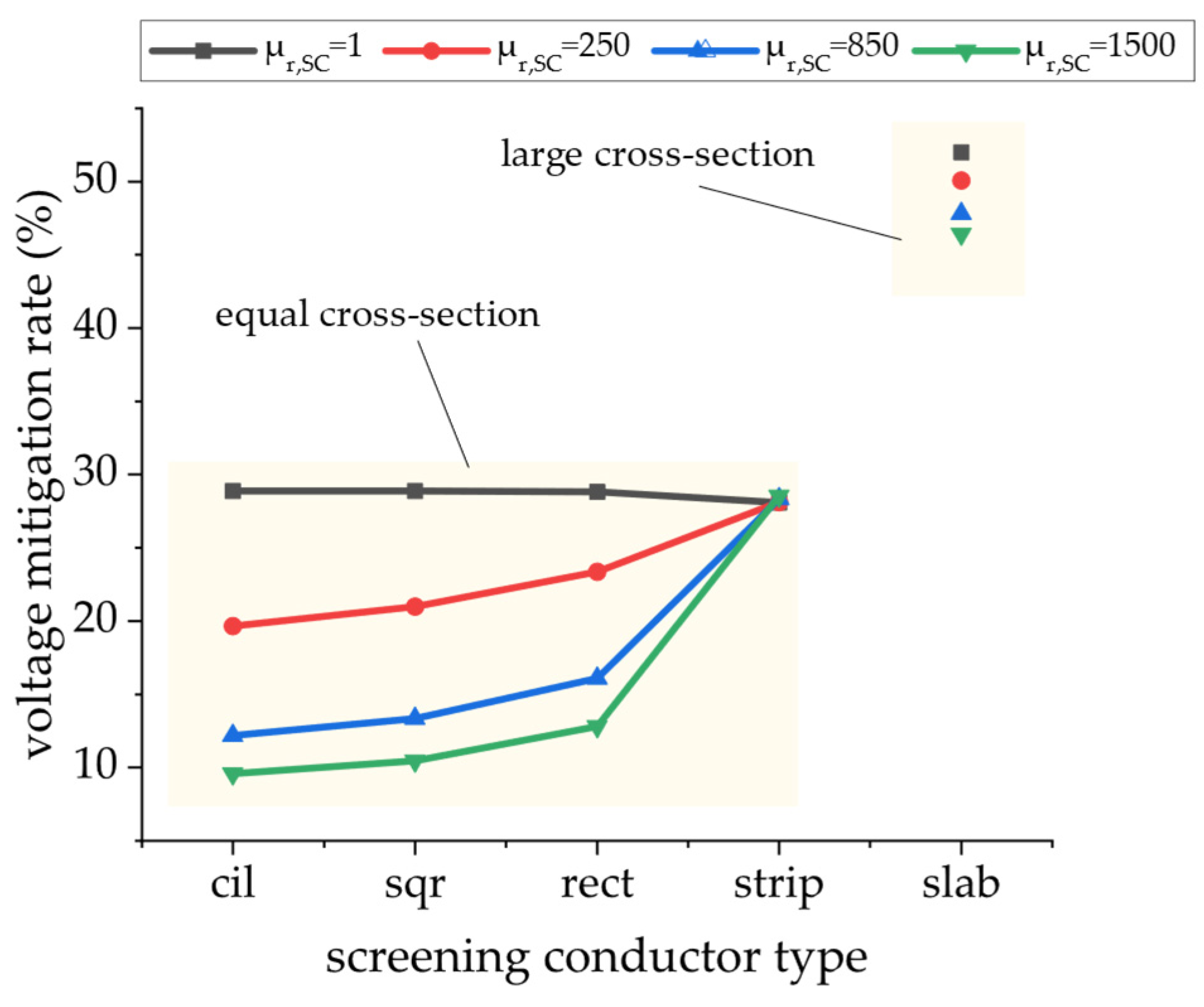
In order to provide a quantitative description of the different mitigation efficacies obtained in the results reported in the previous section, the mitigation rate can be defined for both the induced pipe-to-soil voltage and pipeline current. Considering for example the voltage migration rate, the figure of merit can be defined as:
where is the maximum value of pipeline-to-soil voltage in the considered corridor when no mitigation means are considered.
The computed mitigation rates for both the induced voltage and current, obtained with all the different screening conductor types and values of magnetic permeability described in the previous section, are reported in Figure 13 and Figure 14, respectively.
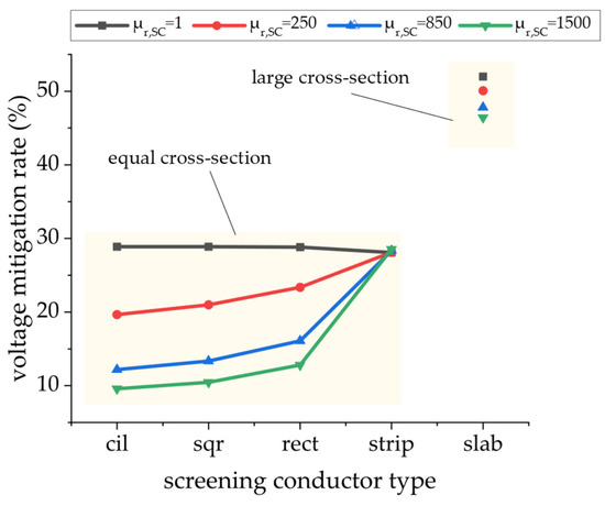
Figure 13.
Voltage mitigation rate for different configurations of the screening conductors; each color corresponds to a different value of , the relative magnetic permeability of the screening conductors; the results corresponding to the slab configuration represent an ideal case, where a considerably larger cross section is employed.
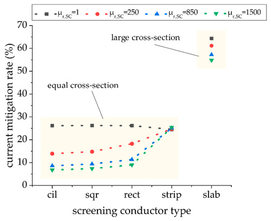
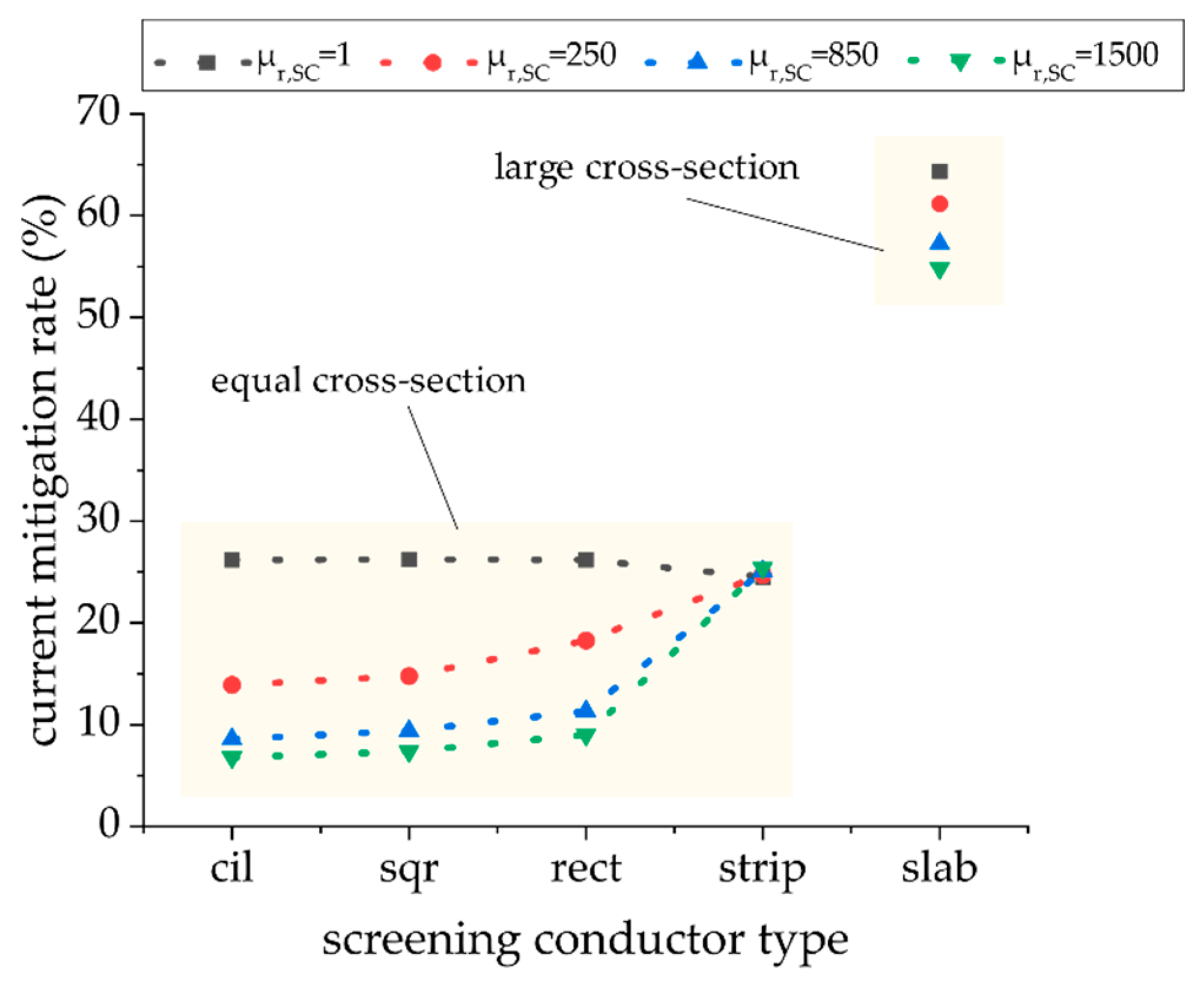
Figure 14.
Current mitigation rate for different configurations of the screening conductors; each color corresponds to a different value of , the relative magnetic permeability of the screening conductors; the results corresponding to the slab configuration represent an ideal case, where a considerably larger cross section is employed.
The mitigating effect of a screen is attributable to two different mechanisms. The first one is due to the electric currents that are induced by the main time varying magnetic field, created by the power line. The currents induced in the screening conductors, in turn, produce a reaction magnetic field that opposes the inducing field. In this respect, an increase of the screening conductor’s magnetic permeability is potentially detrimental, since it causes a skin depth reduction. This may reduce the portion of the conductor crossed by the current, significantly impairing the mitigation rate. The conductor cross-section shape also affects the distribution of the magnetic field produced by the conductor itself. Considering the same current and cross-section area, the magnetic field in close proximity to the conductor is higher for the conductor with the smallest outer perimeter. That is, the same current provides the most efficient local shielding when flowing in a cylindrical conductor, which exhibits the lowest ratio between the outer perimeter and cross-section area. This explains the slight reduction in the mitigation rates observed in Figure 13 and Figure 14 for the strip configuration, with respect to the cyl, sqr, and rect ones, when . Indeed, this is the only case where the current density in the screening conductors is approximately uniform, due to the large skin depth.
A second mechanism exploits the magnetic properties of the material constituting the screen [6]. Indeed, a high-permeability screen constitutes a preferential path for the magnetic field produced by the power line, diverting it away from the pipeline. The obtained results show that—in the cases presented in this paper—the latter mechanism plays little role, since the small size of the screening elements does not reduce significantly the reluctance of the magnetic flux tubes. An exception can be found by observing the behavior of the strip configuration, where an increase of the magnetic permeability does not cause any change in the current induced in the conductor. Still, the voltage mitigation rate slightly increases from 28.1% for to 28.5% for . In this case, the improvement in screening efficiency can be ascribed to the way in which the magnetic properties of the shielding material affect the distribution of the magnetic field lines.
Apart from this case, the screening efficiency is generally dominated by the electric current induced in the screening conductors. As a result, while the voltage and current mitigation rates of the strip screen type do not vary significantly when different values of are considered, marked differences are obtained for the cyl, sqr, and rect configurations. As previously mentioned, this is due to the strip geometrical height, , being smaller than the skin depth in the whole range of relative permeability values.
Conversely, the observed physical behavior changes when a single large slab of steel is employed as a single screening conductor instead of four strip type screening conductors. In particular, as can be observed in Figure 13 and Figure 14, both and show a decrease for increasing values of , just like the cyl, sqr, and rect configurations, but for overall higher values of mitigation rate (due to the markedly larger area of the conductor). This behavior is expected, due to the height of the slab, being larger than the skin depth when .
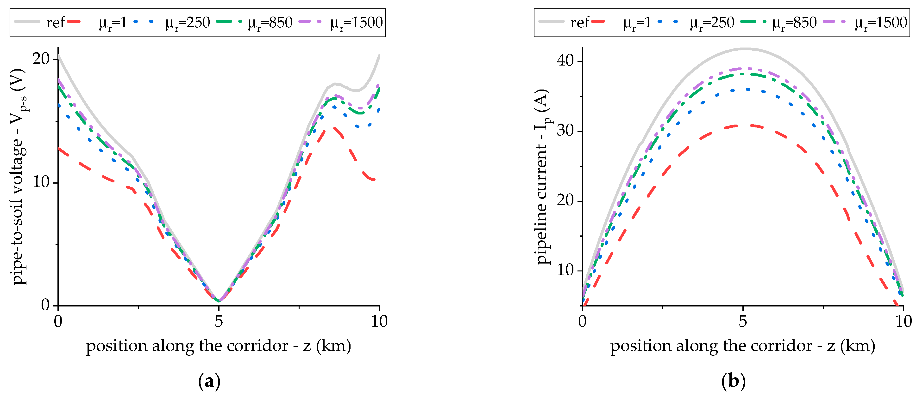
At this point, it its worthwhile to focus on the different behavior yielded by the different screen conductors in relation to the employed magnetic permeability. Figure 15 shows the obtained pipe-to-soil voltage and pipeline current when cylindrical mitigation wires are employed, for different values of the relative magnetic permeability. The results are compared to the unmitigated case (marked in grey color). The figure shows that—for this particular shape—the magnetic permeability exerts a significant influence the mitigation efficacy of the screening conductors. This is somehow an expected result, since (at 50 Hz) even for the penetration depth ( mm) is comparable to the conductor radius (). Therefore, if is increased the consequent reduction of the penetration depth leads to lower currents in the mitigation conductors due to a correspondingly increased impedance.
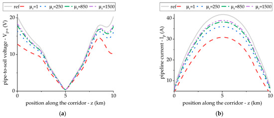
Figure 15.
Induced pipe-to-soil voltage (a) and current (b) along the length of the corridor for different values of relative magnetic permeability () of four cylindrical screening conductors (cyl in Figure 6); the unmitigated results (grey continuous line) are marked as ref.
The comparison between the above discussed results and the ones for the strip shape shows two opposite situations. Indeed, in this second case the penetration depth is considerably smaller than the strip height () in the whole range (1–1500) of magnetic permeability, leading to the observed independence between and the mitigation rate.
As a general note, the results discussed in this work have been obtained by simulating a power line characterized by a symmetric (spatial) disposition of the phase conductors. Assuming equal power line currents—an asymmetric disposition of the conductors would lead to higher magnetic fields and hence higher levels of induced currents and voltages on the power line. Nevertheless, the mitigation efficiency in Equation (10) has been defined as a relative quantity. Hence, the result in terms of screening efficacy would not be affected by the magnitude of the inducing magnetic field, provided that the levels of the induced magnetic fields are low enough to allow the assumption of linearity of the magnetic materials formulated in Section 2.
Finally, the practical consequence of the results reported in this work is that—in general—in order to maximize the mitigation rate non-magnetic steel should be employed for the construction of electromagnetic screens such as the ones considered in this work.
Nevertheless, retaining the same area and electrical conductivity for the screening conductors, the adoption of strip-like shapes, i.e., conductors characterized by a height smaller than then the skin depth, allows the employment of cheaper magnetic steels, while retaining the same mitigation performances that can be obtained using non-magnetic steels.
5. Conclusions
In this work an investigation aimed at highlighting how the shape and magnetic properties of a shielding conductor affect its mitigation efficiency was presented. The considered application is the mitigation of electromagnetic interference induced by a high-voltage power line on a metallic pipeline sharing the same corridor.
The numerical study was conducted through a quasi-3D finite element analysis. Mitigation was achieved using four steel conductors, buried at a fixed depth above the pipeline. Keeping the same cross-sectional area, different shapes and magnetic permeabilities have been considered, and the obtained shielding performances have been compared and discussed.
Results have shown that the magnetic properties of the material used for the screening elements do not directly produce any substantial modifications in the distribution of the magnetic field lines. The mitigation efficiency is mainly determined by the currents that are induced in the screening conductors. As a result, an increase of the magnetic permeability causes a decrease of the active cross section of the cylindrical, square, and rectangular conductors, determining a performance decay. Conversely, the increase of the magnetic permeability does not negatively affect the performance of the strip-shaped conductors, their height being smaller than the skin depth in all the considered conditions. This suggests that an appropriate choice of the screening element cross section allows the use of cheaper magnetic steel, keeping the performance of the device unaltered. Hence, in general, higher values of magnetic permeability are expected to produce lower screening efficiencies unless, as suggested by the strip configuration results, an appropriate choice is made for the screening conductors shape, i.e., maximizing the perimeter-to-area ratio.
Author Contributions
Conceptualization, A.P., A.C. and L.S.; methodology, A.C. and A.P.; software, A.P. and A.C.; validation, A.P., A.C. and L.S.; formal analysis, A.C.; investigation, A.P.; resources, A.C., L.S.; data curation, A.P.; writing—original draft preparation, A.P.; writing—review and editing, A.P., A.C. and L.S.; visualization, A.P.; supervision, A.C. All authors have read and agreed to the published version of the manuscript.
Funding
This research received no external funding.
Institutional Review Board Statement
Not applicable.
Informed Consent Statement
Not applicable.
Data Availability Statement
Not applicable.
Conflicts of Interest
The authors declare no conflict of interest.
Appendix A
Each of the 27 corridor sections marked in Figure 4 has been discretized by means of a 2D triangular mesh, obtained using the GMSH software [28]. Each section has a circular shape, with the boundary condition enforced on the outer edge. The top part of the mesh contains the aerial power line, whereas the bottom part corresponds to the soil, containing the pipeline and the screening conductors. In this study, the soil electrical conductivity has been set to , yielding a skin depth of . The mesh radius has accordingly been set to 10 km.
For what concerns the implementation of the proposed methodology, the 2D finite element solver employed to extract the characteristic matrices from the sections of the corridor was implemented by the authors in Fortran 90 language. The code employs the Intel MKL PARDISO library to solve the sparse complex linear system stemming from the magnetic vector potential equation discretization over 2D triangular meshes. The tableau analysis routine—used to solve the equivalent circuit embodying the physical information extracted with FEA—has been implemented in MATLAB, since the computational load is considerably lower compared to the finite element solver.
References
- Peabody, A.W.; Verhiel, A.L. The Effects of High-Voltage AC Transmission Lines on Buried Pipelines. IEEE Trans. Ind. Gen. Appl. 1971, IGA-7, 395–402. [Google Scholar] [CrossRef]
- Dabkowski, J.; Taflove, A. Prediction Method for Buried Pipeline Voltages Due to 60 Hz AC Inductive Coupling Part II–Field test Verification. IEEE Trans. Power Appar. Syst. 1979, PAS-98, 788–794. [Google Scholar] [CrossRef]
- Lucca, G. AC interference from a faulty power line on nearby buried pipelines: Influence of the surface layer soil. IET Sci. Meas. Technol. 2020, 14, 225–232. [Google Scholar] [CrossRef]
- Micu, D.D.; Christoforidis, G.C.; Czumbil, L. AC interference on pipelines due to double circuit power lines: A detailed study. Electr. Power Syst. Res. 2013, 103, 1–8. [Google Scholar] [CrossRef]
- Ruan, W.; Southcy, R.D.; Tee, S.; Dawalibi, F.P. Recent advances in the modeling and mitigation of AC interference in pipelines. In Proceedings of the NACE-International Corrosion Conference Series; Nace International: Nashville, TN, USA, 2007; pp. 76521–765210. [Google Scholar]
- Gomes, N.; Almeida, M.E.; Machado, V.M. Series Impedance and Losses of Magnetic Field Mitigation Plates for Underground Power Cables. IEEE Trans. Electromagn. Compat. 2018, 60, 1761–1768. [Google Scholar] [CrossRef]
- Corrosion of Metals and Alloys-Determination of AC Corrosion-Protection Criteria; Standard EN ISO 18086:2017; International Organization for Standardization: Geneva, Switzerland, 2017.
- Abdel-Gawad, N.M.K.; El Dein, A.Z.; Magdy, M. Mitigation of induced voltages and AC corrosion effects on buried gas pipeline near to OHTL under normal and fault conditions. Electr. Power Syst. Res. 2015, 127, 297–306. [Google Scholar] [CrossRef]
- Ouadah, M.; Touhami, O.; Ibtiouen, R.; Benlamnouar, M.F.; Zergoug, M. Corrosive effects of the electromagnetic induction caused by the high voltage power lines on buried X70 steel pipelines. Int. J. Electr. Power Energy Syst. 2017, 91, 34–41. [Google Scholar] [CrossRef]
- Bortels, L.; Parlongue, J.; Fieltsch, W.; Segall, S. Manage Pipeline Integrity by Predicting and Mitigating HVAC Interference. In Proceedings of the NACE-International Corrosion Conference Series; Nace International: San Antonio, TX, USA, 2010; pp. 1–15. [Google Scholar]
- Al-Badi, A.H.; Ellithy, K.; Al-Alawi, S. Prediction of voltages on mitigated pipelines paralleling electric transmission lines using ANN. Int. J. Comput. Appl. 2010, 32, 15–22. [Google Scholar]
- Dabkowski, J. How to predict and mitigate A. C. voltages on buried pipelines. Pipeline Gas J. 1979, 206, 19–21. [Google Scholar]
- Tachick, H. AC mitigation using shield wires and decoupling devices. Mater. Perform. 2008, 47, 36–39. [Google Scholar]
- Popoli, A.; Cristofolini, A.; Sandrolini, L.; Abe, B.T.; Jimoh, A. Assessment of AC interference caused by transmission lines on buried metallic pipelines using F.E.M. In Proceedings of the 2017 International Applied Computational Electromagnetics Society Symposium, Firenze, Italy, 26–30 March 2017. [Google Scholar] [CrossRef]
- Ametani, A.; Yoneda, T.; Baba, Y.; Nagaoka, N. An Investigation of Earth-Return Impedance Between Overhead and Underground Conductors and Its Approximation. IEEE Trans. Electromagn. Compat. 2009, 51, 860–867. [Google Scholar] [CrossRef]
- Lucca, G. Mutual impedance between an overhead and a buried line with earth return. In Proceedings of the Ninth International Conference on Electromagnetic Compatibility, Wroclaw, Poland, 13–17 September 2010; (Conf. Publ. No. 396). pp. 80–86. [Google Scholar]
- Kaboli, A.; Hr, S.; Al Hinai, A.; Al-Badi, A.; Charabi, Y.; Al Saifi, A. Prediction of Metallic Conductor Voltage Owing to Electromagnetic Coupling Via a Hybrid ANFIS and Backtracking Search Algorithm. Energies 2019, 12, 3651. [Google Scholar] [CrossRef] [Green Version]
- Popoli, A.; Sandrolini, L.; Cristofolini, A. A quasi-3D approach for the assessment of induced AC interference on buried metallic pipelines. Int. J. Electr. Power Energy Syst. 2019, 106, 538–545. [Google Scholar] [CrossRef]
- Popoli, A.; Sandrolini, L.; Cristofolini, A. Inductive coupling on metallic pipelines: Effects of a nonuniform soil resistivity along a pipeline-power line corridor. Electr. Power Syst. Res. 2020, 189, 106621. [Google Scholar] [CrossRef]
- CIGRE. Guide on the Influence of High Voltage AC Power Systems on Metallic Pipelines; Cigré Working Group 36.02: Paris, France, 1995. [Google Scholar]
- Cristofolini, A.; Popoli, A.; Sandrolini, L. Numerical Modelling of Interference from AC Power Lines on Buried Metallic Pipelines in Presence of Mitigation Wires. In Proceedings of the 2018 IEEE International Conference on Environment and Electrical Engineering and 2018 IEEE Industrial and Commercial Power Systems Europe (EEEIC/I&CPS Europe), Palermo, Italy, 12–15 June 2018; pp. 1–6. [Google Scholar]
- Popoli, A.; Sandrolini, L.; Cristofolini, A. Finite Element Analysis of Mitigation Measures for AC Interference on Buried Pipelines. In Proceedings of the 2019 IEEE International Conference on Environment and Electrical Engineering and 2019 IEEE Industrial and Commercial Power Systems Europe (EEEIC/I&CPS Europe), Genoa, Italy, 11–14 June 2019; pp. 1–5. [Google Scholar]
- Popoli, A.; Cristofolini, A.; Sandrolini, L. A numerical model for the calculation of electromagnetic interference from power lines on nonparallel underground pipelines. Math. Comput. Simul. 2020. [Google Scholar] [CrossRef]
- Steele, C.W. Numerical Computation of Electric and Magnetic Fields; Springer Science & Business Media: New York, NY, USA, 2012. [Google Scholar]
- Hayashi, T.; Mizuno, Y.; Naito, K. Study on Transmission-Line Arresters for Tower with High Footing Resistance. IEEE Trans. Power Deliv. 2008, 23, 2456–2460. [Google Scholar] [CrossRef]
- Yadee, P.; Premrudeepreechacharn, S. Analysis of Tower Footing Resistance Effected Back Flashover across Insulator in a Transmission System. In Proceedings of the International Conference on Power Systems Transients, Lyon, France, 4–7 June 2007. [Google Scholar]
- ITU-T. CCITT Directives Volume {III}: Calculating Induced Voltages and Currents in Pratical Cases; ITU-T: Geneva, Switzerland, 1989. [Google Scholar]
- Geuzaine, C.; Remacle, J.-F. Gmsh: A three-dimensional finite element mesh generator with built-in pre- and post-processing facilities. Int. J. Numer. Methods Eng. 2009, 79, 1309–1331. [Google Scholar] [CrossRef]

Publisher’s Note: MDPI stays neutral with regard to jurisdictional claims in published maps and institutional affiliations. |
© 2021 by the authors. Licensee MDPI, Basel, Switzerland. This article is an open access article distributed under the terms and conditions of the Creative Commons Attribution (CC BY) license (https://creativecommons.org/licenses/by/4.0/).