Shading and Masking of PV Collectors on Horizontal and Sloped Planes Facing South and North—A Comparative Study

Abstract

With the increase in PV system installations, the available free land and rooftops for these systems may become scarcer, and therefore sloped fields facing the north may be utilized for that purpose. In deployments of PV collectors in multiple rows, either on horizontal or sloped planes, the second and subsequent rows are subject to two effects: shading and masking. Both effects reduce the electric energy generated by the PV systems. Multiple rows of collectors are deployed on horizontal planes and on sloped planes facing south, and literature on the topic has been published. No literature deals analytically with deployments of PV fields on north-facing slopes in the northern hemisphere, to the best of our knowledge. The present study develops explicit analytical expressions for the shadow height and length cast on a collector row by a row in front in multiple-row PV systems installed on slopes facing north. In addition, analytical expressions are developed for row spacing and sky view factors, altogether leading consequently to the determination of shading and masking losses. Having the developed expressions, a comparison was made between PV deployments on north-facing sloped planes to PV deployments on horizontal and south-facing slopes regarding shading and masking losses. The main finding is that the percentage of masking losses (diffuse radiation) may exceed the percentage of shading losses (beam radiation) in PV fields. At the local site ${32}^{\circ } \mathrm{N}$, collector inclination angle $\beta ={25}^{\circ }$ and sloped-plane $\epsilon ={10}^{\circ }$, for example, the percentage of masking losses for a horizontal plane is 6.90%; for a sloped plane facing south, the losses are 5.39%, and for a sloped plane facing north, the losses are 6.86%. In comparison to the masking losses, the percentage of shading losses for the horizontal plane is 0.83%; for the sloped plane facing south, the losses are 0.42%, and for the sloped plane facing north, the losses are 1.37%.

1. Introduction

Photovoltaic (PV) energy as a sustainable source of energy is among the renewable low-carbon resources having scalability features and reaching technological maturity. As a fast-growing energy technology, photovoltaic energy will contribute vastly to the global increase in electricity for years to come. With the increase in the number and size of PV system installations, the land becomes a player in the triangle relation between electricity consumption, PV electricity production and land use [1,2]. To mitigate the land-use issue, building-integrated photovoltaics (BIPVs) including rooftops are widely used where electricity consumption is in proximity with electricity production, avoiding energy distribution losses. In addition, dual uses of land have applications in agrivoltaic systems where energy production is associated with crop growing, known as land-integrated photovoltaics (LIPVs) [2]. As free land available for PV systems is becoming scarcer, sloped fields facing the north may be utilized for that purpose. Photovoltaic fields are usually deployed in multiple collector rows with a row-to-row distance. The PV collectors in the second and in the subsequent rows are subject to shading and masking (obscuring), both of which reduce the incident solar radiation and, as a result, reduce the electric energy generated by the PV field. Shading on a second row by a front row affects the direct beam incident radiation, and masking the second row by a front row affects the diffuse incident radiation. Masking reduces the view angle of a collector to the sky, known as the sky view factor. Both shading and masking are dependent on field and collector parameters. These two effects have technical significance implications because the design of a PV system is based on the module’s rated power for all modules in the PV field. The investigation on shading by adjacent collector rows deployed on horizontal surfaces and its effect on solar PV systems started early in [3]. The calculation of global radiation on rows tilted toward the equator on a horizontal surface is presented in [4] considering shading and masking. A mathematical model for shading calculation is developed in [5] for a multiple row deployment of PV collectors on a horizontal surface. A mathematical formulation of the shading effect is presented in [6] and used to investigate shading for three possible collectors’ orientations: fixed-tilt, full-tracking and half-tracking. The effect of row distance shading on the output of PV modules is reported in [7]. References [8,9] follow the above studies and include step-like structures and sloped grounds facing south. The study in [8] is an extension to [3] and deals with the analytical formulation of shading on PV collectors deployed on horizontal and step-like collectors (equivalent to sloped surfaces) facing south. The shadow geometry for horizontal and inclined solar fields facing south is presented in [9] for different types of solar fields. Studies on row distances in PV systems are presented in [10,11,12], as row distance affects the amount of shading. Reference [10] proposes a method that optimizes the minimization of the distance between rows, which is of particular interest for stand-alone PV systems. In [11], a vector analysis method is used to determine the spacing between rows, and the results are validated by comparing with a ray-tracing method. Optimal row spacing taking into account economic factors such as land purchase and preparation and wiring costs is dealt with in [12]. Masking (expressed by sky view factor) that affects the diffuse incident radiation on collectors was considered later in time in [13,14,15]. The study in [13] emphasizes the difference in the amounts of incident diffuse radiation on a top and a bottom module installed on a collector due to the difference in the sky view factors. Various types of view factors to the sky, between opposite collectors, between collector and shaded and unshaded grounds and for front and rear sides of collectors were developed in [14]. The work in [15] analyses the sky view factor for isotropic and anisotropic diffuse and albedo radiation. The effect of shading and masking on optimized PV system deployments is dealt with in [16] for horizontal and sloped fields. Numerous articles, including [17,18], to mention a few, investigate the effect of non-uniform solar radiation on the PV module’s electrical output power resulting from shading and masking on the PV modules. The study in [17] outlines a model for evaluating the extent to which steps are induced on a PV module I-V curve as a direct result of the view-factor variations across the module’s surface. In [18], a method is presented for inter-row shading to calculate irradiance distribution along the width of the PV rows using the Hay transposition model for diffuse, circumsolar and ground-reflected irradiance components.

The studies above on shading and masking have been published for horizontal and south-facing sloped planes (in the northern hemisphere), providing analytical expression for row spacing, shadow height and length, view factors and shading losses. No literature deals analytically with the deployment of PV fields on north-facing slopes in the northern hemisphere, to the best of our knowledge. North-facing sloped fields and north-facing sloped rooftops may be economically utilized for PV energy generation depending on the gradient of the slopes. The contribution of the present study is in developing explicit analytical expressions for the shadow height, length and area cast on a collector row by a row in front in a multiple-row sloped-PV field facing north. In addition, analytical expressions are developed for row spacing and sky view factors, altogether leading consequently to the determination of the shading and masking losses. Having the developed expressions for north sloped fields, comparing the shading and masking losses of PV systems deployed on horizontal and sloped fields facing south to PV systems on north slopes is of interest and is performed. The study pertains to latitude ${32}^{\circ } \mathrm{N}$ (Tel Aviv, Israel) and is based on hourly solar radiation data from the Israel Meteorological Service (IMS). The main finding is that the percentage of masking losses (diffuse radiation) amounts to several percent, whereas the percentage of shading losses (beam radiation) is around 1%. The percentage losses are calculated by the difference between yearly incident solar diffuse and beam radiations on the first row (not subject to losses) and the second (subject to losses) rows. The study relates to mono-facial PV collectors.

2. Materials and Methods

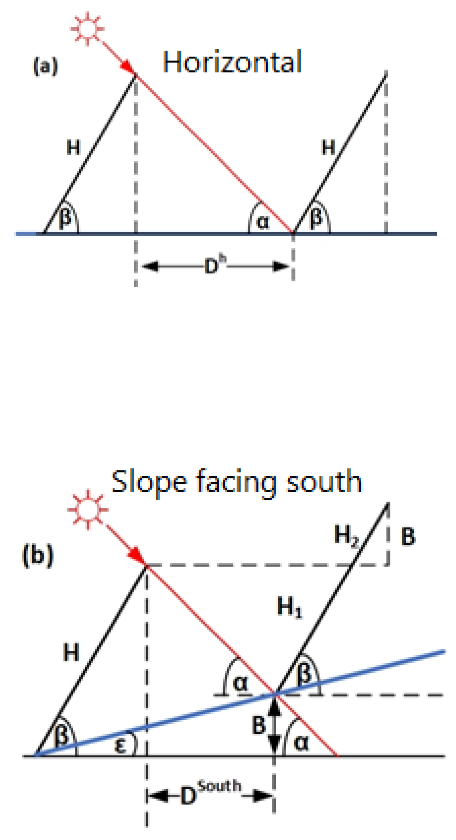
Shading and masking on collectors occur on the second and subsequent rows in PV fields, resulting in generated energy losses. These losses are dependent on field and collector parameters, latitude and solar radiation.

2.1. Row Distance

Figure 1a depicts a horizontal deployment of two collectors facing south of width $H$ and inclination angle $\beta$ and separated by a distance $D^h$. Collectors facing south deployed on a south sloped-plane $\epsilon$ and separated by row distance $D^{south}$ are shown in Figure 1b, and collectors facing south deployed on a north sloped-plane $\epsilon$ separated by $D^{north}$ are depicted in Figure 1c. The sun elevation angle is $\alpha$.

The row distance in PV fields is customarily determined by the shadow length on 21 December at solar noon (see Figure 1) for which the sun elevation angle $\alpha$ [19] is given by $\sin \alpha =\sin \varphi \sin {\delta }_0+\cos \varphi \cos {\delta }_0$ or

$$\tan \alpha =\tan [{\sin }^{-1}(\cos (\varphi -{\delta }_0))]$$

(1)

where $\varphi$ is the site latitude and δ₀ is sun declination angle at solar noon on 21 December.

2.1.1. Horizontal Plane

A deployment of two collectors on a horizontal plane is shown in Figure 1a.

From the figure, we obtain ($h$ for horizontal): $\tan \alpha =\frac{H\sin \beta }{D^h}$, i.e.,

$$D^h=\frac{H\sin \beta }{\tan \alpha }$$

(2)

Therefore, the row distance between the collectors on a horizontal plane $D^h$ becomes:

$$D^h=\frac{H\sin \beta }{\tan [{\sin }^{-1}(\cos (\varphi -{\delta }_0))]}$$

(3)

2.1.2. South Sloped Plane

A deployment of two collectors on a south sloped-plane $\epsilon$ is shown in Figure 1b. From the figure, we obtain:

$$\tan \alpha =(H\sin \beta -B)/D_{\epsilon }^{south}$$

(4)

By substituting Equation (1) into Equation (4), we obtain:

$$D_{\epsilon }^{south}=\frac{H\sin \beta -B^{south}}{\tan [{\sin }^{-1}(\cos (\varphi -{\delta }_0))]}$$

(5)

where

$$B^{south}=(H\cos \beta +D_{\epsilon }^{south})\tan \epsilon$$

(6)

and substituting Equation (6) into Equation (5) we obtain:

$$D_{\epsilon }^{south}=\frac{H\sin \beta -H\cos \beta \tan \epsilon }{\tan [{\sin }^{-1}(\cos (\varphi -{\delta }_0))]+\tan \epsilon },\hspace{1em}\hspace{1em}\hspace{1em}\epsilon \le \beta$$

(7)

By comparing Equation (3) with Equation (5) (or Equation (7)), we see that the row distance for a south-facing slope is shorter as compared to the row distance for a horizontal plane: $D_{\epsilon }^{south}=D^h\frac{H\sin \beta -B^{south}}{H\sin \beta }<D^h$.

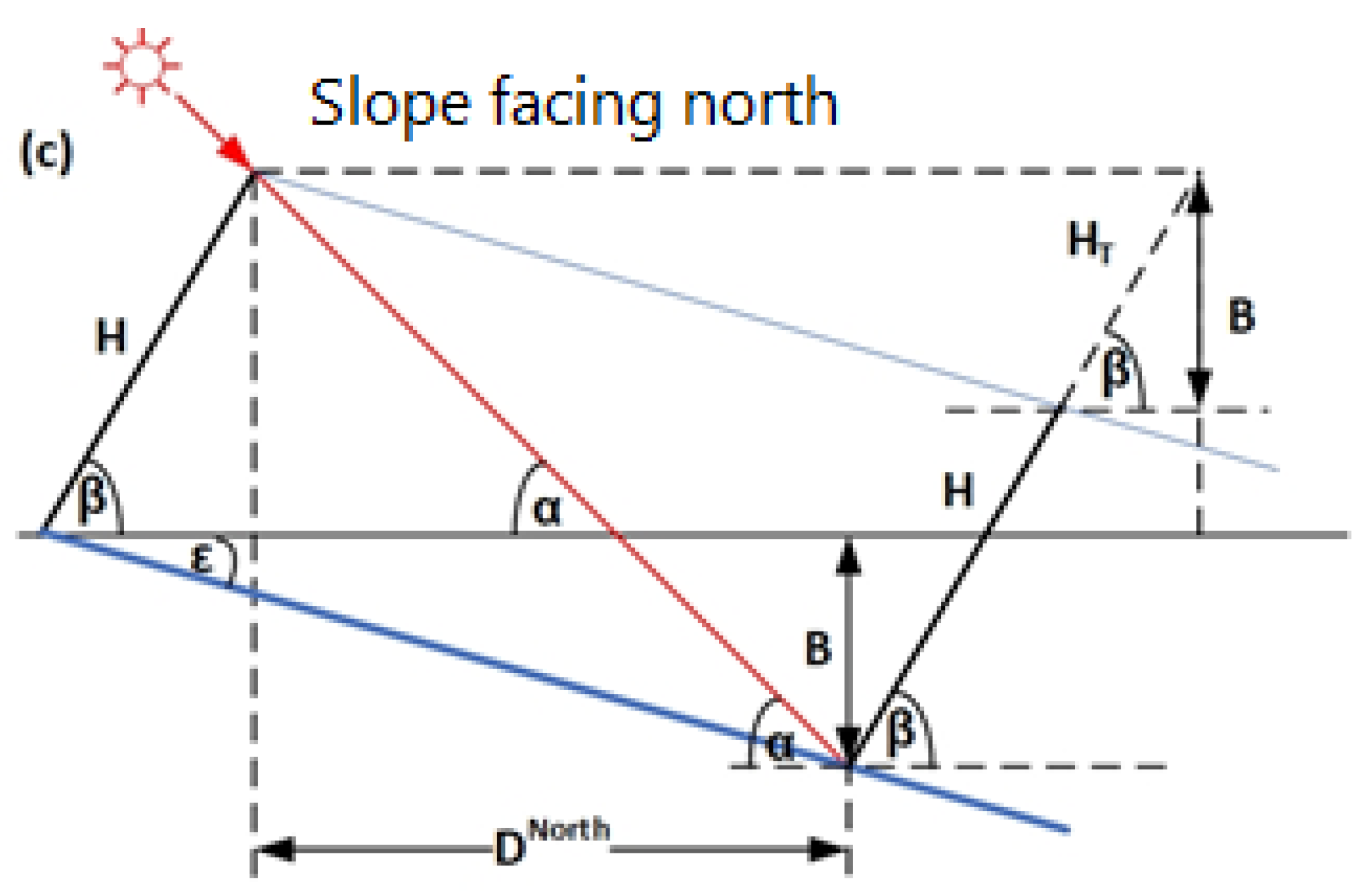
2.1.3. North Sloped Plane

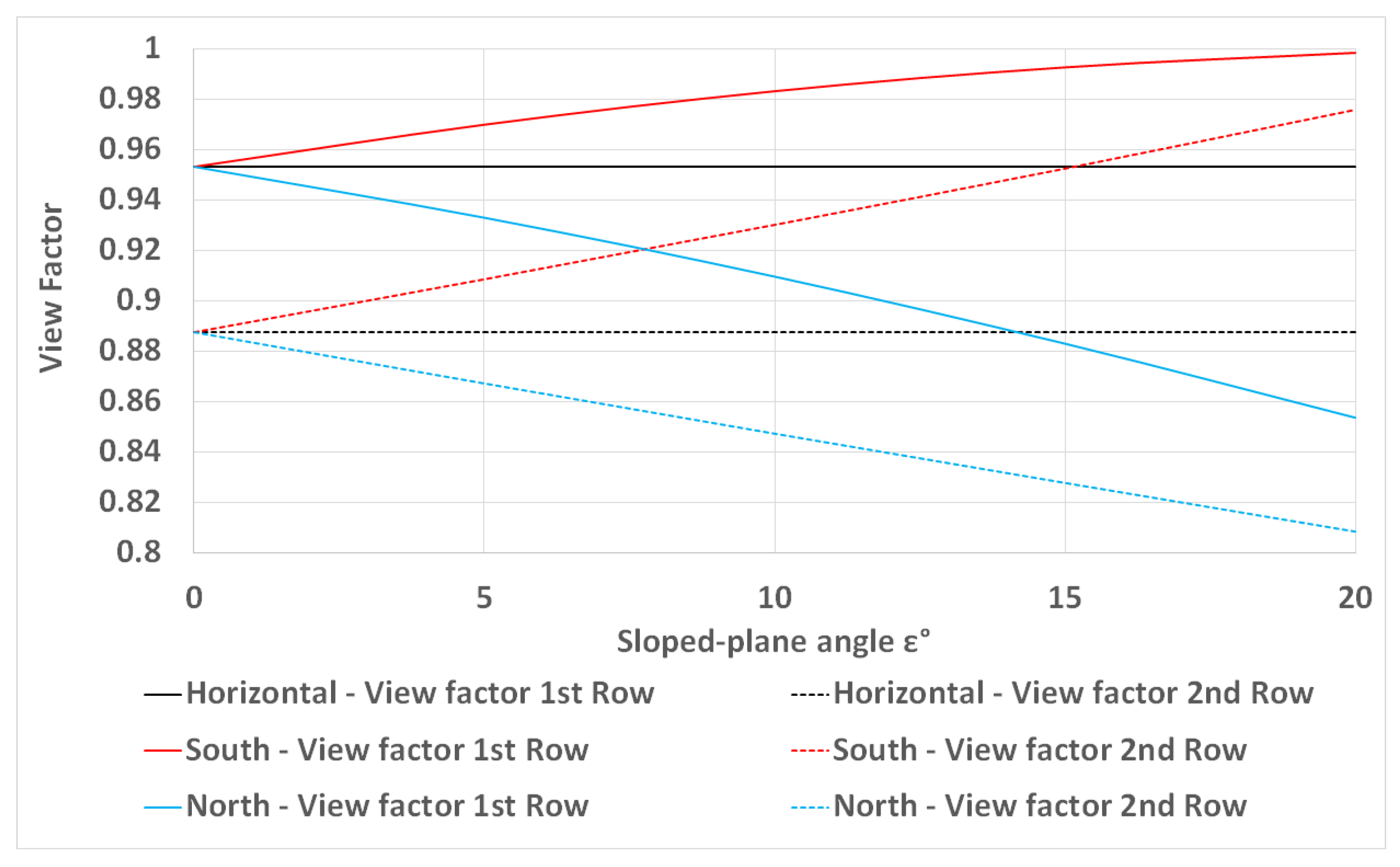
A deployment of two collectors on a north sloped-plane $\epsilon$ is shown in Figure 1c. From the figure we obtain:

$$\tan \alpha =(H\sin \beta +B^{north})/D_{\epsilon }^{north}$$

(8)

$$B^{north}=(H\cos \beta +D^{north})\tan \epsilon$$

(9)

and substituting Equation (9) into Equation (8) we obtain:

$$D_{\epsilon }^{north}=\frac{H\sin \beta +H\cos \beta \tan \epsilon }{\tan [{\sin }^{-1}(\cos (\varphi -{\delta }_0))]-\tan \epsilon },\hspace{1em}\hspace{1em}\hspace{1em}\hspace{1em}\epsilon <{\alpha }_{Dec.21}\hspace{1em}$$

(10)

By comparing Equation (3) with Equation (8) (or Equation (10)) we see that the row distance for a north-facing slope is larger as compared to the row distance for a horizontal plane: $D_{\epsilon }^{north}=D^h{\frac{H\sin \beta +B}{H\sin \beta }}^{north}>D^h$.

The analysis shows that north-facing planes require the widest row spacing (distance) between the collectors as compared to horizontal and sloped planes facing south; i.e., the deployment of the collectors in PV fields on north sloped planes is less dense. The variation of the row distance (see Equations (3), (7) and (10)) with the sloped-plane angle $\epsilon$ is depicted, for example, in Figure 2 for $H=2.12\mathrm{m},\beta ={25}^{\circ },\varphi ={32}^{\circ } \mathrm{N}$.

3. View Factors

Masking (obscuring part of the sky) of a collector row by a row in front is expressed by the sky view factor and is a numerical value depending on the collector width $H$, collector inclination angle $\beta$, distance between the collector rows $D$ and plane slope $\epsilon$. The diffuse radiation collected by a PV collector is coupled with the collector sky view factor and may constitute a large portion of the global radiation. View factors in PV fields on horizontal and sloped planes facing south are dealt with in [13,14]. The sky view factors for the first (front) row on a horizontal plane ${}^1{F}^h$, on a sloped plane facing south ${}^1{F}_{\epsilon }^{south}$ and on a sloped plane facing north ${}^1{F}_{\epsilon }^{north}$ are given by: ${}^1{F}^h=(1+\cos \beta )/2,{}^1{F}_{\epsilon }^{south}=[1+\cos (\beta -\epsilon )]/2,{}^1{F}_{\epsilon }^{north}=[1+\cos (\beta +\epsilon )]/2$.

Based on the “cross-string rule” by Hottel [20], the sky view factor for the second and subsequent rows in a multiple-row PV field deployed on a horizontal plane is given by:

$$F^h=\frac{H+D+H\cos \beta -{[D^2+{(H\sin \beta )}^2]}^{1/2}}{2H}$$

(11)

The sky view factor for a sloped plane facing south is:

$$F_{\epsilon }^{south}=\frac{H+{[{(D_{\epsilon }^{south}+H\cos \beta )}^2+{(B^{south})}^2]}^{1/2}-{[{(D_{\epsilon }^{south})}^2+{(H\sin \beta -B^{south})}^2]}^{1/2}}{2H}$$

(12)

where $B^{south}$ is given in Equation (6), and the sky view factor for a sloped plane facing north is:

$$F_{\epsilon }^{north}=\frac{H+{[{(D_{\epsilon }^{north}+H\cos \beta )}^2+{(B^{north})}^2]}^{1/2}-{[{(D_{\epsilon }^{north})}^2+{(H\sin \beta +B^{north})}^2]}^{1/2}}{2H}$$

(13)

where $B^{north}$ is given in Equation (9).

The variations of the view factors (see Equations (11)–(13)) with the slope angle $\epsilon$ are depicted in Figure 3, for example, for $H=2.12\mathrm{m},\beta ={25}^{\circ },\varphi ={32}^{\circ } \mathrm{N}$, and for the appropriate row distances $D^h,D_{\epsilon }^{south},D_{\epsilon }^{north}$ (see Equations (3), (7) and (10).

Percentage of Masking Losses

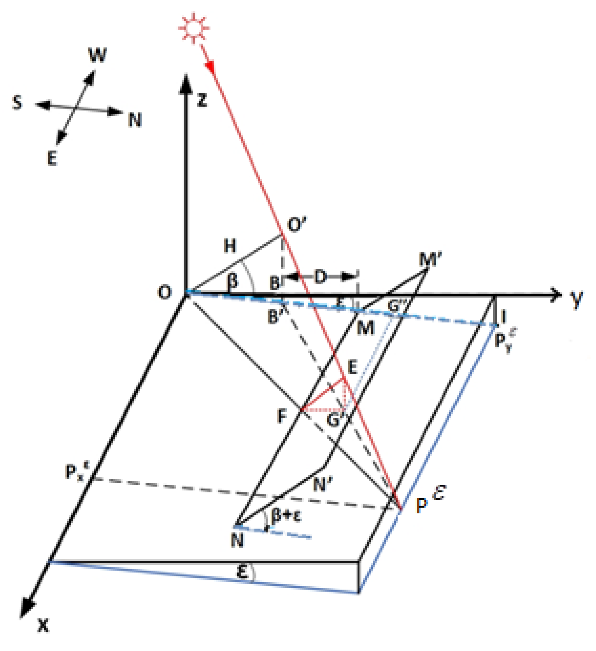
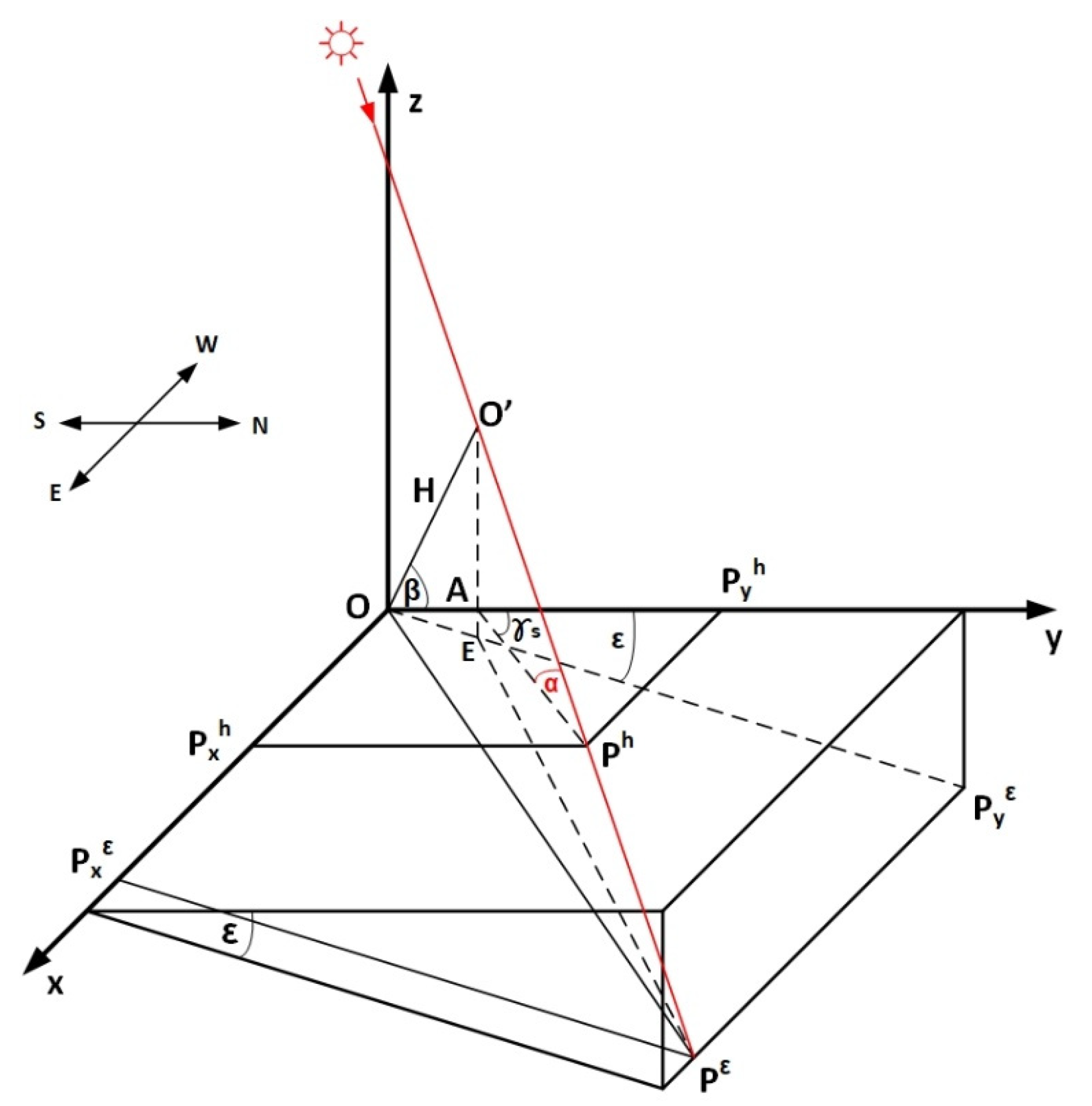
The amount of masking losses is determined by the difference between the annual diffuse incident radiation on the first and on the second row and based on the solar radiation data at Tel Aviv. Figure 4 depicts the ratio of the diffuse radiation between the second and first rows. The ratio pertains to horizontal and sloped-plane $\epsilon$ facing south and north for PV field deployments for $H=2.12\mathrm{m},L=40\mathrm{m}$, $\beta ={20}^{\circ },{25}^{\circ },{30}^{\circ }$ and for the appropriate row distances $D^h,D_{\epsilon }^{south},D_{\epsilon }^{north}$. An isotropic diffuse radiation model is used for the calculations. For example, the percentages of masking losses for a horizontal plane are 5.48% ($\beta ={20}^{\circ }$), 6.90% ($\beta ={25}^{\circ }$) and 8.33% ($\beta ={30}^{\circ }$). In terms of energy losses, 5.48% (for $\beta ={20}^{\circ }$ and horizontal plane) amounts to a yearly masking loss of $36.7\mathrm{kWh}/{\mathrm{m}}^2$ (the horizontal global solar irradiation at the site is 1826 kWh/m²/year). For a south sloped-plane $\epsilon ={10}^{\circ }$, the masking losses are 3.58%, 5.39% and 7.22%, respectively, and for a north sloped plane, the masking losses are 5.83%, 6.86% and 7.92%, respectively. The results show, as expected, that the masking losses increase with the increase in the collector inclination angle $\beta$. The lowest diffuse radiation losses are obtained for deployments on south sloped planes. Actually, the diffuse radiation losses stem from the difference in the view factors of the first and the second collector rows; therefore, the percentage of these losses may be calculated from the sky view factors for the isotropic diffuse radiation model.

4. Shading by Poles

To compute the shadow height, length and area cast on a collector row by a row in front, the shadow components of a pole need to be derived first, as a collector may be considered as composed of an infinite number of poles. At the onset, the shadow components of vertical and inclined poles on horizontal and sloped planes are derived to determine finally the amount of shading on adjacent rows.

4.1. Vertical Pole on a Horizontal Plane

Figure 5 shows a vertical pole of height $H$ at the origin, a horizontal plane and a sloped plane facing north with an angle $\epsilon$. First, we consider a horizontal plane. The sun is in altitude $\alpha$ and in azimuth ${\gamma }_s$. The pole casts a shadow $O{P}^h$ on the horizontal plane, the components of which are:

$$P_y^h=H\frac{\cos {\gamma }_s}{\tan \alpha }$$

(14)

$$P_x^h=H\frac{\sin {\gamma }_s}{\tan \alpha }$$

(15)

4.2. Inclined Pole on Horizontal Plane

The shadow components of an inclined pole with angle $\beta$ in a ($y,z$) plane on a horizontal plane (see Figure 6) are given by:

$$P_x^h=\frac{H\sin \beta \sin {\gamma }_s}{\tan \alpha }$$

(16)

$$P_y^h=\frac{H\sin \beta \cos {\gamma }_s}{\tan \alpha }+H\cos \beta$$

(17)

4.3. Vertical Pole on a Sloped Plane

The pole $H$ (see Figure 5) casts a shadow length $O{P}^{\epsilon }$ on the sloped plane $\epsilon$ with respect to the horizontal plane. The derivation of the shadow length and its components are now calculated. Using the “vector form of the equation of a straight line”, the shadow components $P_x^{\epsilon },P_y^{\epsilon },P_z^{\epsilon }$ of the shadow $O{P}^{\epsilon }$ are now determined. Any straight line in space may be presented by a vector (direction) and a point on the vector. Based on the coordinates of two known points $A(0,0,H)$ and $P^h(P_x^h,P_y^h,0)$ on the horizontal plane, we obtain $P_y^h=H\frac{\cos {\gamma }_s}{\tan \alpha }$, $P_x^h=H\frac{\sin {\gamma }_s}{\tan \alpha }$ and $P_z^h=0$ (see Equations (14) and (15)); thus, a point on the line $A,P^h,P^{\epsilon }$ may be presented by:

$$line:(0,0,H)+t\times (H\frac{\sin {\gamma }_s}{\tan \alpha },H\frac{\cos {\gamma }_s}{\tan \alpha },-H)$$

(18)

where $t$ is a scalar.

The coordinates of point $P^{\epsilon }(P_x^{\epsilon },P_y,P_z^{\epsilon })$ on the line (Equation (18)) are:

$$P_x^{\epsilon }=t\times H\times \frac{\sin {\gamma }_s}{\tan \alpha }$$

(19)

$$P_y=t\times H\times \frac{\cos {\gamma }_s}{\tan \alpha }$$

(20)

$$P_z^{\epsilon }=H\times (1-t)$$

(21)

In addition, from Figure 5 we have:

$$P_z^{\epsilon }/P_y=\tan \epsilon$$

(22)

where for $\epsilon <0$, the slope is facing north, and for $\epsilon >0$, the slope is facing south. Substituting Equations (20) and (21) into Equation (22), we obtain $\frac{H\times (1-t)}{t\times H\times \frac{\cos {\gamma }_s}{\tan \alpha }}=\tan \epsilon$ and solving for $t$ we obtain:

$$t=\frac{\tan \alpha }{\cos {\gamma }_s\tan \epsilon +\tan \alpha },$$

(23)

Therefore, the coordinates of point $P^{\epsilon }(P_x^{\epsilon },P_y,P_z^{\epsilon })$ become:

$$P_x^{\epsilon }=\frac{H\sin {\gamma }_s}{\cos {\gamma }_s\tan \epsilon +\tan \alpha }$$

(24)

$$P_y=\frac{H\cos {\gamma }_s}{\cos {\gamma }_s\tan \epsilon +\tan \alpha }$$

(25)

$$P_z^{\epsilon }=\frac{H\cos {\gamma }_s\tan \epsilon }{\cos {\gamma }_s\tan \epsilon +\tan \alpha }$$

(26)

Finally, point $P_y^{\epsilon }$ is obtained (see Figure 5) by:

$$P_y^{\epsilon }={[{(P_z^{\epsilon })}^2+{(P_y)}^2]}^{1/2}=\frac{H\cos {\gamma }_s}{\cos {\gamma }_s\sin \epsilon +\tan \alpha \cos \epsilon }$$

(27)

4.4. Inclined Pole on a Sloped Plane

The inclined pole $O{O}^{\prime }$ in Figure 6 casts a shadow $O{P}^{\epsilon }$ on a sloped-plane $\epsilon$ facing north. Similar to the derivation of a vertical pole on a sloped plane using the vector form approach, the line $O^{\prime }{P}^{\epsilon }$ is determined by two known points, $O^{\prime }(0,H\cos \beta ,H\sin \beta )$ and $P^h(P_x^h,P_y^h,0)$, where $P_x^h=H\sin \beta \frac{\sin {\gamma }_s}{\tan \alpha }$, $P_y^h=H\sin \beta \frac{\cos {\gamma }_s}{\tan \alpha }+H\cos \beta$ and $P_z^h=0$. Therefore, the line $O{P}^{\epsilon }$ may be represented by:

$$line:(0,H\cos \beta ,H\sin \beta )+t\times (H\sin \beta \frac{\sin {\gamma }_s}{\tan \alpha },H\sin \beta \frac{\cos {\gamma }_s}{\tan \alpha },-H\sin \beta )$$

(28)

where point $P^{\epsilon }$ in question lays on this line; i.e., the coordinates are:

$$P_x^{\epsilon }=t\times H\sin \beta \frac{\sin {\gamma }_s}{\tan \alpha }$$

(29)

$$P_y=t\times H\sin \beta \frac{\cos {\gamma }_s}{\tan \alpha }+H\cos \beta$$

(30)

$$P_z^{\epsilon }=H(1-t)\sin \beta$$

(31)

In addition, $P_z^{\epsilon }/P_y=\tan \epsilon$, and based on Equations (30) and (31), the scalar $t$ may be solved, obtaining:

$$t=\frac{\tan \alpha \sin \beta -\cos \beta \tan \epsilon }{\sin \beta \times [\tan \alpha +\cos {\gamma }_s\tan \epsilon ]}$$

(32)

By substituting $t$ into Equations (29)–(31), the coordinates of point $P_x^{\epsilon },P_y,P_z^{\epsilon }$ become:

$$P_x^{\epsilon }=\left(\frac{\sin \beta -\cos \beta \tan \epsilon }{\sin \beta \times (\tan \alpha +\cos {\gamma }_s\tan \epsilon )}\right)H\sin \beta \sin {\gamma }_s$$

(33)

$$P_y=\left(\frac{\sin \beta -\cos \beta \tan \epsilon }{\sin \beta \times (\tan \alpha +\cos {\gamma }_s\tan \epsilon )}\right)H\sin \beta \cos {\gamma }_s+H\cos \beta$$

(34)

$$P_z^{\epsilon }=H\tan \epsilon \left(\frac{\sin \beta \cos {\gamma }_s+\tan \alpha \cos \beta }{\tan \alpha +\cos {\gamma }_s\tan \epsilon }\right)$$

(35)

where $P_y^{\epsilon }$ is obtained from:

$$P_y^{\epsilon }={\left[{(P_z^{\epsilon })}^2+{(P_y)}^2\right]}^{1/2}$$

(36)

Notice that for $\beta ={90}^{\circ }$, the coordinates of point $P^{\epsilon }$ are reduced to the coordinates of point $P^{\epsilon }$ for a vertical pole on a sloped plane (see Equations (24)–(27)).

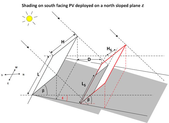
5. Shadow on Collectors

The shadow height $H_s$, length $L_s$ and area ($H_s\times L_s$) on an adjacent collector by a collector in front are now determined for a horizontal plane and for south- and north-facing sloped planes. A deployment of collectors on a north-facing slope is depicted in Figure 7.

5.1. Deployment on a Horizontal Plane

Based on [4], the shadow height $H_s^h$ on the adjacent collector deployed on a horizontal plane is given by:

$$H_s^h=H\left[1-R^h/P_y^h\right]$$

(37)

where $R^h$ (see Figure 1a and Equation (2)) is given by:

$$R^h=D^h+H\cos \beta =\frac{H\sin \beta }{\tan \alpha }+H\cos \beta$$

(38)

and $P_y^h$ is given in Equation (17), resulting in:

$$H_s^h=H\left(1-\frac{D^h+H\cos \beta }{H\cos \beta +H\sin \beta \cos {\gamma }_s/\tan \alpha }\right)$$

(39)

The shadow length is given by [4]:

$$L_s^h=L-R^h\times \frac{P_x^h}{P_y^h}$$

(40)

With Equations (16), (17) and (38), the shadow length results in:

$$L_s^h=L-(D^h+H\cos \beta )\frac{\sin \beta \sin {\gamma }_s/\tan \alpha }{\cos \beta +\sin \beta \cos {\gamma }_s/\tan \alpha }$$

(41)

5.2. Deployment on a Sloped Plane

5.2.1. North-Facing Plane—$\epsilon <0$

Similarly to the case of a horizontal plane, one may prove that the shadow height ${}^{north}{H}_s^{\epsilon }$ on an adjacent collector deployed on a sloped plane facing north is (see Figure 8):

$${}^{north}{H}_s^{\epsilon }=H(1-\frac{R_{north}^{\epsilon }}{{}^{north}{P}_y^{\epsilon }})$$

(42)

where (see Figure 1c and Equation (10)):

$$\begin{array}{l}{R}_{north}^{\epsilon }=(D_{\epsilon }^{north}+H\cos \beta )/\cos \epsilon =\frac{H\sin \beta +H\cos \beta \tan \epsilon }{(\tan \alpha -\tan \epsilon )\cos \epsilon }+\frac{H\cos \beta }{\cos \epsilon }\\ \end{array}$$

(43)

By substituting Equations (10), (36) and (43) in Equation (42), we obtain the shadow height $H_s^{\epsilon }$.

The shadow length is given by using Equations (33), (36) and (43):

$${}^{north}{L}_s^{\epsilon }=L-R_{north}^{\epsilon }\times \frac{{}^{north}{P}_x^{\epsilon }}{{}^{north}{P}_y^{\epsilon }}$$

(44)

and the shaded area is ${}^{north}{H}_s^{\epsilon }{\times }^{north}{L}_s^{\epsilon }$.

Notice that ${}^{north}{P}_x^{\epsilon }$ and ${}^{north}{P}_y^{\epsilon }$ (Equations (33) and (36)) are the coordinates of point ${}^{north}{P}^{\epsilon }$ for $\epsilon <0$, i.e., for a north-facing slope.

5.2.2. South-Facing Plane—$\epsilon >0$

The calculation of the shadow height and length on an adjacent collector deployed on a sloped plane facing south is similar to the calculation on a sloped plane facing north. The results are:

$${}^{south}{H}_s^{\epsilon }=H(1-\frac{R_{south}^{\epsilon }}{{}^{south}{P}_y^{\epsilon }})$$

(45)

where (see Figure 1b):

$$\begin{array}{l}{R}_{south}^{\epsilon }=(D_{\epsilon }^{south}+H\cos \beta )/\cos \epsilon =\frac{H\sin \beta -H\cos \beta \tan \epsilon }{(\tan \alpha +\tan \epsilon )\cos \epsilon }+\frac{H\cos \beta }{\cos \epsilon }\\ \end{array}$$

(46)

By substituting Equations (7), (36) and (46) in Equation (45), we obtain the shadow height $H_s^{\epsilon }$.

The shadow length is given by using Equations (25), (26) and (36):

$${}^{south}{L}_s^{\epsilon }=L-R_{south}^{\epsilon }\times \frac{{}^{south}{P}_x^{\epsilon }}{{}^{south}{P}_y^{\epsilon }}$$

(47)

and the shaded area is ${}^{south}{H}_s^{\epsilon }{\times }^{south}{L}_s^{\epsilon }$.

Notice that ${}^{south}{P}_x^{\epsilon }$ and ${}^{south}{P}_y^{\epsilon }$ (Equations (33) and (36)) are the coordinates of point ${}^{south}{P}^{\epsilon }$ for $\epsilon >0$, i.e., for a south-facing slope.

Figure 9 describes, for example, the variation of the shadow height and length with time on December 21 on a collector in the second row deployed on a horizontal plane and on sloped planes facing south and north with an angle $\epsilon =5^{\circ }$. The collector’s height and length are $2.12\mathrm{m},40\mathrm{m}$, respectively, erected with an inclination angle $\beta ={25}^{\circ }$ at latitude $\varphi ={32}^{\circ } \mathrm{N}$. The row distances corresponding to Equations (3), (7) and (10) are $D^h=1.30\mathrm{m},D_{\epsilon }^{south}=0.94\mathrm{m},D_{\epsilon }^{north}=1.77\mathrm{m}$. The shaded areas are depicted by rectangles; for example, at 9:00 a.m., the shaded areas are $10.9{\mathrm{m}}^2$ for horizontal deployment, $6.4{\mathrm{m}}^2$ for south deployment and $17.9{\mathrm{m}}^2$ for north deployment. North deployment suffers more shading than the other collector deployments.

5.3. Percentage of Shading Losses

The amount of shading losses is determined by the difference in the yearly beam incident radiation on the first and on the second row. Figure 10 depicts the percentage of shading losses (with respect to the first row) for horizontal and sloped planes $\epsilon$ facing south and north, for PV field deployments of $H=2.12\mathrm{m},L=40\mathrm{m}$, $\varphi ={32}^{\circ } \mathrm{N}$; for $\beta ={20}^{\circ },{25}^{\circ },{30}^{\circ }$; and for the appropriate row distances $D^h,D_{\epsilon }^{south},D_{\epsilon }^{north}$. For example, the shading losses for the horizontal plane are 0.68% ($\beta ={20}^{\circ }$), 0.83% ($\beta ={25}^{\circ }$) and 0.98% ($\beta ={30}^{\circ }$).

For a horizontal plane and $\beta ={25}^{\circ }$, 0.83% amounts to a yearly shading loss of $11.2\mathrm{kWh}/{\mathrm{m}}^2$, where the horizontal global solar irradiation at the site is $1826\mathrm{kWh}/{\mathrm{m}}^2/\mathrm{year}$. For a sloped-plane $\epsilon$ facing south, the shading losses are 0.29%, 0.42% and 0.56%, respectively; for a sloped plane facing north, the shading losses are 1.19%, 1.37% and 1.54%, respectively. The results show, as expected, that the shading losses increase with the increase in the collector inclination angle $\beta$.

6. Discussion

The available free land and rooftops for PV systems will become scarcer in the future, and therefore sloped fields facing the north may be utilized for that purpose. Analytical derivation of shading parameters (shadow height, length and area) for a field of PV collectors facing south and deployed on northern sloped planes (in the northern hemisphere) has not been published in the literature. Designing PV systems using various available computer software may have the option of designing PV systems on sloped planes facing the north; however, as the software does not specify the algorithms, one is not able to verify them, introduce modifications and perform different studies at will. The present article develops, step by step, mathematical expressions for shading losses in a PV field deployed on northern slopes. With the above-developed tool, a comparison of the annual shading and masking losses of PV fields is made for horizontal and sloped planes facing south and north. The parameters that govern the losses (in addition to solar radiation) are row spacing, sky view factors, shadow height and length, collector width and inclination angle. For a correct comparison, the row spacing was determined by the same criteria of the shadow length on December 21 for all three cases. As the result, the values of the row spacing are different, and consequently, the sky view factors and the shading and masking losses differ for each case of the PV deployment. The sloped-plane angle $\epsilon$ is limited to $\epsilon \le \beta$ for south slopes and $\epsilon <{\alpha }_{Dec.21}$ for north slopes (${\alpha }_{Dec.21}$ is the sun’s altitude on December 21 at solar noon). At higher latitudes $\varphi$, the utilization of sloped land facing north for PV systems are more limited. The main finding is that the percentage of masking losses amounts to several percent whereas the percentage of shading losses is around 1% for all three cases of land: horizontal, south and north slopes. The percentage losses are calculated by the difference between yearly incident solar diffuse and beam radiations on the first and the second row. Increasing the collector angle results in increasing both the masking and shading losses. The study presented in [16] shows that increasing the row distance has a greater effect on the masking losses than on the shading losses. Reference [16] refers to horizontal and sloped planes facing south; however, with the extension of the present study for north-facing sloped planes, it is plausible to state that the sensitivity of shading losses to row distance is less pronounced than that of masking losses since the row distance is determined by the same criteria for all three cases of land.

7. Conclusions

With the increase in PV system installations, sloped fields facing the north may be utilized for that purpose. In deployments of PV collectors in multiple rows on either horizontal or sloped planes, the second and subsequent rows are subject to two effects: shading and masking. Both effects reduce the electric energy generated by the PV systems. The purpose of the study was to develop analytical expressions for shading and masking losses in PV systems deployed on north-facing slopes and compare them to the shading and masking losses in PV systems deployed on horizontal and south-facing planes. The present paper dealt analytically with three factors to consider in the design of PV fields: row spacing, sky view factors and shadow heights and lengths cast on a collector row by a row in front. The main finding is that masking losses (diffuse radiation) amount to several percent whereas shading losses (beam radiation) are around 1%. The diffuse incident radiation on a PV field at the site of the simulation latitude ${32}^{\circ } \mathrm{N}$ is about 30%, resulting in masking losses exceeding the shading losses. At locations with a higher percentage of diffuse radiation, masking losses may imply more concern. Shading and masking effects have implications of technical significance because the design of a PV system is based on the module’s rated power for all modules in the PV field. PV fields on north-facing slopes require a larger row distance than the other deployments. Shading and masking losses increase with the increase in the collector inclination angle.

References

1. Mancini, F.; Nastasi, B. Solar energy data analytics: PV deployment and land use. Energies 2020, 13, 417. [Google Scholar] [CrossRef] [Green Version]
2. Scognamiglio, A. ‘Photovoltaic landscapes’: Design and assessment. A critical review for a new transdisciplinary design vision. Renew. Sustain. Energy Rev 2016, 55, 629–661. [Google Scholar] [CrossRef]
3. Appelbaum, J.; Bany, J. Shadow effect of adjacent solar collectors in large scale systems. Sol. Energy 1979, 23, 497–508. [Google Scholar] [CrossRef]
4. Jones, R.E., Jr.; Burkhart, J.F. Shading effect of collector row tilt toward the equator. Sol. Energy 1981, 26, 563–565. [Google Scholar] [CrossRef]
5. Budin, R.; Budin, L. A mathematical model for shading calculations. Sol. Energy 1982, 29, 339–349. [Google Scholar] [CrossRef]
6. Groumpos, P.P.; Kouzam, K.Y. A Generic approach to the shadow effect in large solar power systems. Sol. Cells 1987, 22, 29–46. [Google Scholar] [CrossRef]
7. Goswami, D.Y. Effect of Row-to-Row Shading on the Output of Flate South Facing Solar Arrays, Final Report; North Carolina Agricultural & Technical State University: Greensboro, NC, USA, 1986. [Google Scholar]
8. Bany, J.; Appelbaum, J. The effect of shading on the design of a field of solar collectors. Sol. Cells 1987, 20, 201–228. [Google Scholar] [CrossRef]
9. Alsadi, S.Y.; Nassar, Y.F. A general expression for the shadow geometry for fixed mode horizontal, step-like structure and inclined solar field. Sol. Energy 2019, 181, 53–69. [Google Scholar] [CrossRef]
10. Castellno, N.N.; Parra, J.A.G.; Valls-Guirado, J.; Manzono-Agugliaro, F. Optimal displacement of photovoltaic array’s rows using a novel shading model. Appl. Energy 2015, 144, 1–9. [Google Scholar] [CrossRef]
11. Copper, J.K.; Sproul, A.B.; Bruce, A.G. A method to calculate potential system size of photovoltaic arrays in urban environment using vector analysis. Appl. Energy 2016, 161, 11–23. [Google Scholar] [CrossRef]
12. Sanchez-Carbajal, S.; Rodrigo, P.M. Optimum array spacing in grid-connected photovoltaic system considering technical and economic factors. Int. J. Photoenergy 2019, 1486749. [Google Scholar] [CrossRef]
13. Appelbaum, J.; Aronescu, A. The effect of sky diffuse radiation on photovoltaic fields. Renew. Sustain. Energy 2018, 10, 033505. [Google Scholar] [CrossRef]
14. Appelbaum, J. The role of view factors in solar photovoltaic fields. Renew. Sustain. Energy Rev. 2018, 81, 161–171. [Google Scholar] [CrossRef]
15. Arias-Rosales, A.; LeDuc, P.R. Comparing view factor modeling frameworks for the estimation of incident solar energy. Appl. Energy 2020, 277, 115510. [Google Scholar] [CrossRef]
16. Aronescu, A.; Appelbaum, J. The effect of collector shading and masking on optimized PV field designs. Energies 2019, 12, 3471. [Google Scholar] [CrossRef] [Green Version]
17. Peled, A.; Appelbaum, J. The view-factor effect shaping of I-V characteristics. Prog. Photovolt. Res. Appl. 2017. [Google Scholar] [CrossRef]
18. Verga, N.; Mayer, M.J. Model-based analysis of shading losses in ground-mounted photovoltaic power plant. Sol. Energy 2021, 216, 428–438. [Google Scholar] [CrossRef]
19. Duffie, J.A.; Beckman, W.A. Solar Engineering of Thermal Processes; John Wiley and Sons, Inc.: New York, NY, USA, 1991. [Google Scholar]
20. Hottel, H.C.; Sarofin, A.F. Radiative Transfer; McGraw Hill: New York, NY, USA, 1967; pp. 31–39. [Google Scholar]
Figure 1. (a) Collectors deployment on planes (b) horizontal with D h , sloped planes facing south with D s o u t h and (c) sloped planes facing north with D n o r t h , blue lines represent the ground.
Energies 14 03850 g001aEnergies 14 03850 g001b
Figure 2. Variation of row distances with sloped-plane angle ε , β = 25 , H = 2.12   m , ϕ = 32   N .
Energies 14 03850 g002
Figure 3. Variation of sky view factors with sloped plane angle ε , β = 25 , H = 2.12   m ,   ϕ = 32 .
Energies 14 03850 g003
Figure 4. Ratio of diffuse radiation between the second and first rows for sloped plane angles ε , H = 2.12   m ,   L = 40   m , ϕ = 32   N .
Energies 14 03850 g004
Figure 5. Shadow components of a vertical pole on a horizontal plane at point P h and on a northern sloped plane at point P ε .
Energies 14 03850 g005
Figure 6. Shadow components of an inclined pole β on a horizontal plane at point P h and on a southern sloped plane at point P ε .
Energies 14 03850 g006
Figure 7. Shadow on a collector deployed on a north-facing sloped plane ε .
Energies 14 03850 g007
Figure 8. Shadow height E F =   n o r t h H s ε on collector M N M N .
Energies 14 03850 g008
Figure 9. Shadow variation on adjacent collectors for horizontal, south-facing and north-facing planes; β = 25 ,   ε = 5 ,   ϕ = 32   N ,   H = 2.12   m ,   L = 40   m ,   December   21 .
Energies 14 03850 g009
Figure 10. Percentage of shading losses between the first and second collector row; H = 2.12   m ,   L = 40   m ,   ϕ = 32   N , β = 20 ,   25 ,   30 .
Energies 14 03850 g010
Publisher’s Note: MDPI stays neutral with regard to jurisdictional claims in published maps and institutional affiliations.