Measurement Method of Thermal Diffusivity of the Building Wall for Summer and Winter Seasons in Poland

Abstract

The thermal diffusivity of building materials is an extremely important parameter influencing the subsequent thermal comfort of building users. By definition, thermal diffusivity describes how quickly heat from a hot source can flow through a material. Therefore, this parameter includes both the thermal conductivity and the heat capacity of the material. This parameter is often neglected in heat-related calculations which, in the case of dynamic problems, leads to unreliable results. It should be taken into account that heat flows through all materials at a finite speed. On the other hand, knowing the correct thermal diffusivity value of building materials, it is possible to accurately determine the internal parameters in rooms over time. There are several methods for determining thermal diffusivity, most of which are destined to determine this property in laboratories. The aim of the present research is to show how the thermal diffusivity of materials can be determined in existing buildings. The presented method can be used to determine more real thermal parameters used for thermal calculations in buildings, for example, during energy audits or when calculating the demand for cooling for air conditioning or heat for space heating. This research presents the results for a 60 cm brick wall. Thermal diffusivity was determined for specific summer and winter days—most representative of the whole year. This research has shown that the applied method should be used in the summer period, due to the fact that the wall has greater temperature fluctuations. The obtained results are comparable with the previously mentioned laboratory methods. However, due to the fact that the materials analyzed on the spot, the results are more reliable, and also take into account changes in the value of thermal diffusivity resulting from the use of binders, inaccuracies in joining and external layers made of other materials.

1. Introduction

Building materials comprise a large group of substances. Among them are thermal insulations with a thermal conductivity of $\lambda =0.02$ W/(m·W), materials that conduct heat well, such as metals with a conductivity coefficient of several hundred W/(m·K) and intermediate materials. The $c_p$—specific heat value also covers a wide range from 200 to 1000 J/(kg·K).

In turn, the coefficient of thermal diffusivity is a parameter that determines the speed of heat propagation in the body in the way of conduction [1,2]. It depends on the conductivity but also on the heat capacity of the material. Thermal conductivity characterizes the flow of conducted heat, and capacity characterizes the amount of energy that must be supplied by or received from a given part of the sample to change its temperature by a certain amount. Thus, diffusivity is an essential parameter in the analysis of non-stationary heat conduction. Thermal diffusivity is defined as [3]

$$a=\frac{\lambda }{\rho ·c_p},$$

(1)

where: a is thermal diffusivity (m${}^2$/s), $\lambda$ is thermal conductivity (W/m·K), $\rho$ is density (kg/m${}^3$) and c${}_p$ is specific heat (J/(kg·K)). Usually, materials with high thermal conductivity also have a high density, which limits the variability of thermal diffusivity. Comparing the most insulating materials with the best heat-conducting materials, a thermal diffusivity value of a = 1.54 × 10${}^{-7}$ m${}^2$/s can be obtained for aerogel insulation [4], and a = 1.00 × 10${}^{-4}$ m${}^2$/s for steel [5]. However, the lowest diffusivity value should not be pre-assigned to the best insulation and the highest should not be pre-assigned to the best heat conductor.

This article deals with the measurements of the thermal diffusivity of a wall made of mineral materials such as bricks and concrete. Based on the results of the works [6,7,8], the thermal diffusivity of concrete covers the range 5.090 × 10${}^{-8}$–1.283 × 10${}^{-5}$ m${}^2$/s. Concrete is a material with a large variety of components and as such it has wide range of possible values of this parameter [9,10]. The thermal diffusivity of a brick wall, obtained from [11,12,13] is in the range of 0.35 × 10${}^{-6}$–3.34 × 10${}^{-6}$ m${}^2$/s. Knowledge of thermal diffusivity values can also be used to evaluate other physical properties. By measuring the thermal diffusivity, it is possible to determine the hardness of steel [5] or the physical properties of new nanomaterials [14].

For building materials, thermal diffusivity often depends on moisture saturation [15,16]. For concrete, the ability to absorb water depends not only on the composition but also on the proportion of ingredients [17]. For bricks, the change of moisture saturation causes a 200% change in the value of the thermal conductivity coefficient and a 70% change in thermal effusivity [18].

Most of the methods for determining the thermal diffusivity coefficient consist of measuring the temperature of the tested sample during variable heat flow. The phenomenon of changing the heat flux is forced artificially in the laboratory or is the result of natural processes. Many methods compare the change in the measured temperature on the surface of the sample material with the change in temperature obtained as a result of calculations for known boundary conditions. A review of the methods based on the periodic boundary condition is presented in publication [19]. The Ångstrom method [20,21,22] is the most popular in this case. For this application, the measurement of two parameters characterizing non-stationary heat transfer is required; phase shift and amplitude decay with distance from the periodic boundary condition [23,24]. By analyzing the response of the sample to periodic extortion, it is even possible to determine the thermal properties of a multi-layer material [25,26,27,28]. The method based on the stepwise variability of the boundary condition was discussed in publications [11,29].

The next group of methods for determining thermal diffusivity is the use of variable natural conditions. In these studies, it was decided to use this method. This solution allows the obtaining of the thermal diffusivity in the place where the sample is located and where the heat flow directly influences the conformation of a building’s users. In the experiment, the outside wall’s temperature is influenced by solar radiation, air temperature, air humidity, wind speed and the occurrence of rainfall. In this study, the method for determining thermal diffusivity based on the approximation of the temperature measured in the wall has been presented. It was assumed that the approximating function satisfies the Fourier equation and the thermal diffusivity was determined by solving the inverse problem. Calculations were made for the selected summer and winter day. This parameter was then determined using the Ångström method. This method is based on measurements of amplitude and temperature phase difference. The advantages of this method are its simplicity of use, and its well-established correct operation, confirmed by many works. Based on the measurements made, this method could be directly applied. The Ångström method uses the entire month of August for summer and January for winter as the measuring time. The results of both methods were convergent. Finally, a summary is provided and conclusions are drawn.

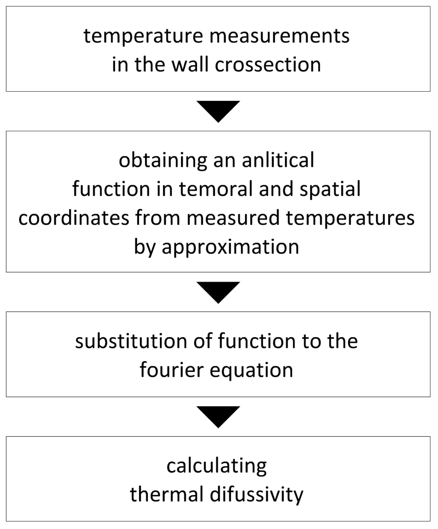
2. Method Description

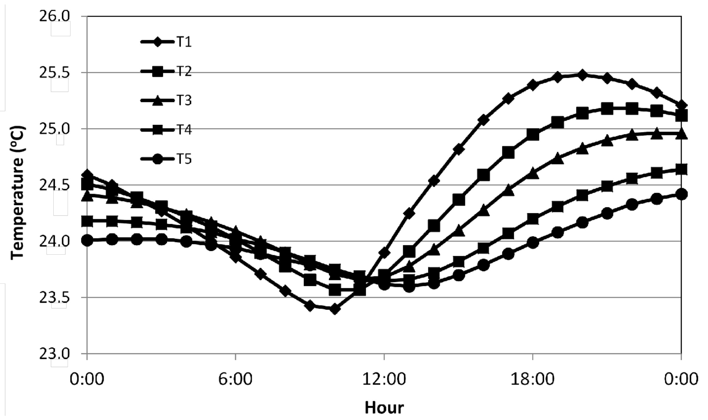
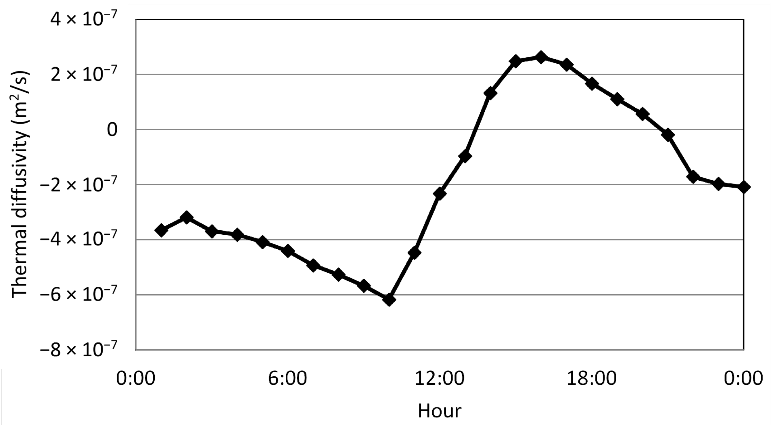
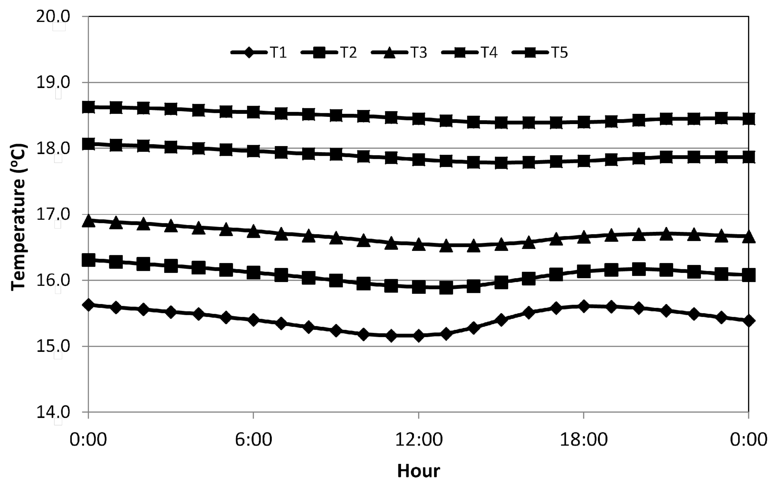
The method described in [30] was used to measure the thermal diffusivity for a selected wall over a period of six months. Figure 1 shows the procedure for the used method.

The measuring apparatus described in detail in [30,31] was used. Temperature sensors were placed in the wall of the existing building. The wall was 0.6 m thick and made of bricks. The distance of the wall temperature sensors from the side walls, ceiling and floor was so large that the heat flow was assumed to be one dimensional. The outer surface of the tested wall was exposed to natural weather conditions. In the experimental study, Pt1000 temperature sensors were used. The stand is shown in Figure 2.

The phenomenon of heat transport by conduction is described by the Fourier equation:

$$\frac{\partial T}{\partial t}=a\frac{{\partial }^{2}T}{\partial x^2},$$

(2)

where the coefficient a is called the thermal diffusivity.

In this analysis, it was assumed that the polynomial equation, which reflects the solution of Equation (2) with sufficient accuracy, has the following form:

$$T(x,t)=p00+p10·x+p01·t+p20·x^2+p11·x·t+p02·t^2,$$

(3)

where x is the wall depth position and t represents time. Equation (2) can be transformed into [32]:

$$a=\frac{\frac{\partial T}{\partial t}}{\frac{{\partial }^{2}T}{\partial x^2}}.$$

(4)

By finding the time and position derivatives from Equation (3), Equation (4) can be written as

$$a=\frac{p01+p11·x+2·p02·t}{2·p20}.$$

(5)

The coefficients shown in Equation (5) ($p00,p10,p01,p20,p11$ and $p02$) have been determined experimentally according to the T1–T5 temperature measurements in the tested wall. For the purposes of approximation, the whole day was divided into 24 patches. The breakdown is presented in Figure 3. Each patch lasts one hour and 10 min. They were defined so that the next patch overlaps the previous 10 min. Patch 3 was continued up to the 180th minute and patch 24 began in the 1380th, not shown in the picture.

Coefficients were calculated in the MATLAB Curve Fitting Toolbox application [33]. In configuration 24, thermal diffusivity values were obtained for each day. In the ideal case, all values are equal across the whole day, neglecting the thermal diffusivity change according to the temperature and moisture saturation changes in the wall. Since the described method is based on natural changes in wall temperature, there is the problem of choosing the right time of day to obtain the most accurate results. The article specifies the most favourable time of the day for carrying out measurements, assuming the criterion of the repeatability of the results.

3. Results

Two days were selected as representations of the summer and winter seasons. For the summer season it was 9 August 2019 and for the winter season it was 3 February 2020. Both days are close to mid-meteorological summer or winter and were cloudless. The calculations were made with the division of the day as shown in Figure 2. The calculated thermal diffusivity for 9 August 2019 is summarized in

Table 1. Thermal diffusivity obtained for 9 August 2019.

Patch no.	1	2	3	4	5	6
a (m${}^2$/s)	4.50 × 10${}^{-7}$	5.71 × 10${}^{-7}$	5.36 × 10${}^{-7}$	6.10 × 10${}^{-7}$	6.39 × 10${}^{-7}$	6.76 × 10${}^{-7}$
Patch no.	7	8	9	10	11	12
a (m${}^2$/s)	6.81 × 10${}^{-7}$	6.94 × 10${}^{-7}$	6.77 × 10${}^{-7}$	5.77 × 10${}^{-7}$	6.91 × 10${}^{-9}$	3.01 × 10${}^{-6}$
Patch no.	13	14	15	16	17	18
a (m${}^2$/s)	1.36 × 10${}^{-6}$	1.22 × 10${}^{-6}$	1.30 × 10${}^{-6}$	1.31 × 10${}^{-6}$	1.29 × 10${}^{-6}$	1.36 × 10${}^{-6}$
Patch no.	19	20	21	22	23	24
a (m${}^2$/s)	1.60 × 10${}^{-6}$	2.48 × 10${}^{-6}$	2.75 × 10${}^{-5}$	−1.10 × 10${}^{-6}$	−4.53 × 10${}^{-8}$	2.07 × 10${}^{-7}$

and for 3 February 2020 in

Table 2. Thermal diffusivity obtained for 3 February 2020.

Patch no.	1	2	3	4	5	6
a (m${}^2$/s)	−3.66 × 10${}^{-7}$	−3.19 × 10${}^{-7}$	−3.69 × 10${}^{-7}$	−3.82 × 10${}^{-7}$	−4.09 × 10${}^{-7}$	−4.41 × 10${}^{-7}$
Patch no.	7	8	9	10	11	12
a (m${}^2$/s)	−4.93 × 10${}^{-7}$	−5.27 × 10${}^{-7}$	−5.67 × 10${}^{-7}$	−6.18 × 10${}^{-7}$	−4.48 × 10${}^{-7}$	−2.33 × 10${}^{-7}$
Patch no.	13	14	15	16	17	18
a (m${}^2$/s)	−9.63 × 10${}^{-8}$	1.33 × 10${}^{-7}$	2.48 × 10${}^{-7}$	2.63 × 10${}^{-7}$	2.37 × 10${}^{-7}$	1.67 × 10${}^{-7}$
Patch no.	19	20	21	22	23	24
a (m${}^2$/s)	1.11 × 10${}^{-7}$	5.65 × 10${}^{-8}$	−1.87 × 10${}^{-8}$	−1.71 × 10${}^{-7}$	−1.97 × 10${}^{-7}$	−2.09 × 10${}^{-7}$

.

The obtained thermal diffusivity values were analyzed as a relation to the outside wall temperature change during a given day. Figure 4 shows the data from Table 1. Each patch represents another hour of the day. In Figure 4, the value for patch 21 is not shown, because this is the moment when a slight change in temperature occurred, and thus the error in determining thermal diffusivity is large (thus the result was more than ten times different than the results for the other patches).

The recorded temperature change from which the diffusivity was determined is shown in Figure 5. It is a typical temperature variation for a sunny summer day for a wall exposed to direct sunlight. Thus, it can be concluded that the shape of the determined thermal diffusivity value is also characteristic for the summer period.

Comparing Figure 4 with Figure 5, it can be concluded that there is a rapid change in the determined value of thermal diffusivity at the moment of the beginning of the morning temperature rise and then the evening temperature drop in the wall. These spikes are caused by the variability of both the solar radiation and the air temperature during the day. The problem of temperature variability in a non-steady state in a massive wall was also investigated in publications [34,35,36].

The examined wall shows large inertia in relation to the ambient temperature variability. The influence of solar radiation is more pronounced. The tested wall has the SE azimuth, therefore it is best irradiated in the morning and early afternoon hours. Since the measuring probes are located in about half of the wall, there is a delay similar to that of solutions with sinusoidal variability of boundary conditions [37]. Between the rapid changes, the value determined from subsequent measurements remains very stable. A different value is obtained for the night–morning period and a different value for the afternoon period. The reason for these differences is probably the different direction of heat flow in the wall. In the night and morning period it is related to the cooling down of the wall and in the afternoon to the heating up.

The second set of the calculated thermal diffusivity patterns is characteristic of the autumn–winter season, a representation of this season is 3 February 2020. Results are shown in Figure 6.

The recorded temperature change inside the wall, from which the thermal diffusivity was determined, is shown in Figure 7.

The temperature during the day shows a small variability and the calculated thermal diffusivity is sinusoidal with disturbances. This is also the typical temperature pattern for a winter day. The negative value of diffusivity is caused by the negative value of the time gradient of the temperature in the night and early afternoon hours.

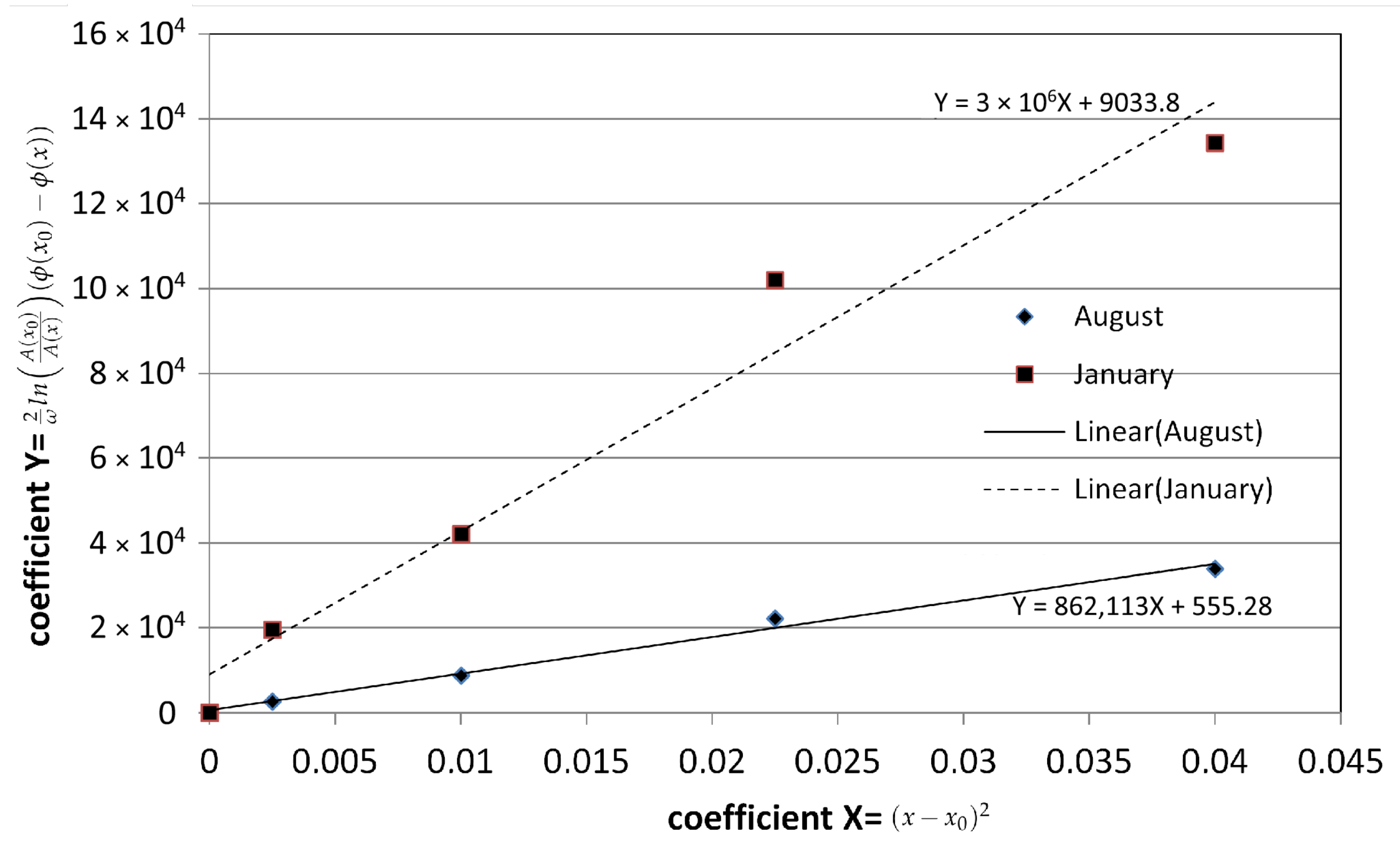
Comparison to the Modified Ångström’s Method

The Ångström method allows us to determine the thermal diffusivity on the basis of the phase shift and amplitude attenuation at a given distance from the boundary condition for the heat flow described by Equation (6)

$$\frac{\partial T}{\partial t}=a\frac{{\partial }^{2}T}{\partial x^2}+\frac{PR}{\lambda A}(T-T_0),$$

(6)

where T is temperature (${}^{\circ }$C), x is the distance inside the wall (m), a is the thermal diffusivity of the wall (m${}^2$/s), t is the time (s), A is the cross-sectional area of the sampled wall (m${}^2$), P is the perimeter of the area A (m), R is the heat loss term, which accounts for both radiation and convection (W/(m${}^2$·K)), $\lambda$ is the thermal conductivity (W/(m·K)), and $T_0$ is the ambient temperature (${}^{\circ }$C). Compared to Equation (2), there is a term related to heat losses to the external environment, but it is not important for the diffusivity calculation. Integrating Equation (6), the basic relation of the Ångström method can be obtained [38,39]:

$$a=\frac{\omega {(x_2-x_1)}^2}{2\varphi ln\left(\frac{A_1}{A_2}\right)},$$

(7)

where $\omega$ is the angular frequency of temperature variation, $(x_2-x_1)$ is the distance between measurement points, and $\varphi$ and $A_1/A_2$ are the phase difference and product of amplitudes at these points, respectively. In publication [40], Equation (7) is presented as

$$\frac{2}{\omega }ln\left(\frac{A\left(x_0\right)}{A\left(x\right)}\right)\left(\varphi \left(x_0\right)-\varphi \left(x\right)\right)=\frac{1}{a}{(x-x_0)}^2.$$

(8)

The point T1 was assumed to be $x_0$, making the assumption that:

$$X={(x-x_0)}^2,$$

(9)

and

$$Y=\frac{2}{\omega }ln\left(\frac{A\left(x_0\right)}{A\left(x\right)}\right)\left(\varphi \left(x_0\right)-\varphi \left(x\right)\right).$$

(10)

$X,Y$ coefficients can be determined for each measurement point. After plotting the points in these coordinates, it is possible to obtain a line the slope of which is the inverse of thermal diffusivity. Using MATLAB, an FFT transform of the temperature record was made for the measured months. Then, the phase and amplitude of a harmonic with frequency 1.157 × 10${}^{-5}$ Hz (T = 24 h), where $\omega$ = 7.272 × 10${}^{-5}$, were read for all points [19]. The obtained values are summarized in

Table 3. Amplitude and phase for the component within a period of 24 h for August 2019 at measurement points.

Measurement Point	Amplitude A	Phase $\mathit{\varphi } \left(\mathbf{rad}\right)$
T1	1298.1	0.578
T2	981.0	0.246
T3	760.3	−0.020
T4	541.3	−0.343
T5	419.5	−0.512

and

Table 4. Amplitude and phase for the component within a period of 24 h for January 2020 at measurement points.

Measurement Point	Amplitude A	Phase $\mathit{\varphi } \left(\mathbf{rad}\right)$
T1	233.3	0.602
T2	161.8	0.236
T3	119.4	−0.064
T4	72.5	−0.708
T5	66.3	−1.064

.

According to assumptions, the X and Y coefficients were calculated and are shown in Figure 8.

The results obtained from both methods are summarized in

Table 5. Thermal diffusivity values for the considered days.

Temperature Profile Method	9 August 2019	3 February 2020
Avg	9.15 × 10${}^{-7}$	2.95 × 10${}^{-7}$
Max	1.60 × 10${}^{-6}$	6.18 × 10${}^{-7}$
Min	4.50 × 10${}^{-7}$	1.87 × 10${}^{-8}$
$\Delta a_{Max-Min}$	1.15 × 10${}^{-6}$	5.99 × 10${}^{-7}$
Ångström method	1.16 × 10${}^{-6}$ (whole August)	3.33 × 10${}^{-7}$ (whole January)

. The mean results of the method proposed in the article were determined, excluding values from the minimum and maximum peaks for the summer day as unrepresentative. On a winter day, the absolute value of all results was taken into account.

The accuracy of the temperature measurement in the wall depends not only on the accuracy of the sensor itself, but also on the contact of the sensor with the wall. This is influenced by the porosity of the wall and the accuracy of the hole for the sensor. This type of problem can be seen in the publications of Habib et al. [41], where the authors introduced the BRT index, which is the quotient of the square of the brick thickness and the corresponding thermal diffusivity; this index changes with the change in the volume of air spaces in the brick for the same dimension (and said spaces are the result of poorly made holes for the sensors). The existence of space affects the diffusivity of the wall. A typical brick wall had about 25% greater thermal resistance than a wall with air voids removed, while having a lower heat capacity. In the experimental tests carried out, the wells were tightly filled with insulating foam, thanks to which the temperature measurement was correct.

Figure 9 shows the ranges of the thermal diffusivity obtained from the literature and previous studies of the authors. It can be seen that the consistency of the results for the wall is satisfactory, especially when comparing with the results obtained for concrete bricks in the literature.

4. Conclusions

The summer period seems to be a better time for measuring thermal diffusivity with the presented method. The obtained diffusivity values are more stable, apart from the temperature solstices occurring twice a day. The best time for measurements is the period from 02:00 to 09:00 and from 14:00 to 18:00. In winter, the obtained values are subject to constant fluctuations. At the same time, taking into account the absolute value, the daily variability for winter is lower than for the summer period. However, the resulting negative value creates problems of interpretation. The values obtained from the Ångström method are close to those obtained with the method proposed in the article, and also show different values in summer and winter. The lower value of diffusivity in winter is probably the result of the temperature distribution in the wall being closer to the steady state. In the steady state, the temperature is constant over time, so the heat capacity of the material does not affect heat propagation. Thus, thermal diffusivity cannot be determined in this condition. The presented method is so much better than other methods as it determines the thermal diffusivity for a real building partition, and it does not matter what material and what layers the partition is made of. It has to be remembered that building partitions not only have different layers, but can also be made of the same materials in a better or worse way. Thus, the results obtained with this method will allow more realistic thermal calculations for a measured building wall. As part of the research, it was not possible to determine the influence of wall moisture on the thermal diffusivity coefficient. This is due to the fact that, on the one hand, moisture increases the thermal conductivity coefficient and, on the other hand, it also increases the density of the material. It is difficult to clearly define which of the parameters is dominant. On the other hand, the wall is exposed to external atmospheric conditions, and the outside temperature fluctuation does not always coincide with the fluctuation of humidity.

The diffusivity values for concrete have a wide range because concrete is a material with a different physical and chemical composition. Research on bricks shows a much narrower scope. The wall studied by the authors shows values in the lower range for bricks and concrete. The obtained results show little variability in relation to the obtained ranges in the literature.

References

1. Salazar, A. On thermal diffusivity. Eur. J. Phys. 2003. [Google Scholar] [CrossRef]
2. Baryłka, A.; Tomaszewicz, D. Influence of measuring deviations of the components of layered walls on their durability. Inż. Bezpieczeństwa Obiektów Antropog. 2020. [Google Scholar] [CrossRef]
3. Carslaw, H.S.; Jeager, J.C. Conduction of Heat in Solids, 2nd ed.; Clarendon Press: Oxford, UK, 1986. [Google Scholar]
4. Lakatos, Á. Comprehensive thermal transmittance investigations carried out on opaque aerogel insulation blanket. Mater. Struct. 2017. [Google Scholar] [CrossRef]
5. Boubaker, K.M.; Bouhafs, M.; Yacoubi, N. A quantitative alternative to the Vickers hardness test based on a correlation between thermal diffusivity and hardness—Applications to laser-hardened carburized steel. NDT&E Int. 2003, 36. [Google Scholar] [CrossRef]
6. Noh, H.G.; Lee, J.H.; Kang, H.C.; Park, H.S. Effective Thermal Conductivity and Diffusivity of Containment Wall for Nuclear Power Plant OPR1000. Nucl. Eng. Technol. 2017, 49, 459–465. [Google Scholar] [CrossRef]
7. Asadi, I.; Shafigh, P.; Bin Abu Hassan, Z.F.; Mahyuddin, N.B. Thermal conductivity of concrete—A review. J. Build. Eng. 2016. [Google Scholar] [CrossRef]
8. Pomianowski, M.; Heiselberg, P.; Jensen, R.L.; Cheng, R.; Zhang, Y. A new experimental method to determine specific heat capacity of inhomogeneous concrete material with incorporated microencapsulated-PCM. Cem. Concr. Res. 2014, 55. [Google Scholar] [CrossRef]
9. Łasica, W.; Małek, M.; Szcześniak, Z.; Owczarek, M. Characterization of recycled glass-cement composite: Mechanical strength. Mater. Tehnol. 2020. [Google Scholar] [CrossRef]
10. Małek, M.; Jackowski, M.; Życiński, W.; Łasica, W.; Owczarek, M. Influence of silicone carbide additions on the mechanical properties of concrete. Mater. Technol. 2019. [Google Scholar] [CrossRef]
11. Azhary, E.; Raefat, S.; Laaroussi, N.; Garoum, M. Energy performance and thermal proprieties of three types of unfired clay bricks. Energy Procedia 2018, 147. [Google Scholar] [CrossRef]
12. Sassine, E.; Younsi, Z.; Cherif, Y.; Chauchois, A.; Antczak, E. Experimental determination of thermal properties of brick wall for existing construction in the north of France. J. Build. Eng. 2017. [Google Scholar] [CrossRef]
13. El Fgaier, F.; Lafhaj, Z.; Brachelet, F.; Antczak, E.; Chapiseau, C. Thermal performance of unfired clay bricks used in construction in the north of France: Case study. Case Stud. Constr. Mater 2015. [Google Scholar] [CrossRef]
14. Fujisawa, H.; Ryu, M.; Lundgaard, S.; Linklater, D.P.; Ivanova, E.P.; Nishijima, Y.; Juodkazis, S.; Morikawa, J. Direct Measurement of Temperature Diffusivity of Nanocellulose-Doped Biodegradable Composite Films. Micromachines 2020, 11, 738. [Google Scholar] [CrossRef]
15. Stolarska, A.; Strzałkowski, J. The Thermal Parameters of Mortars Based on Different Cement Type and W/C Ratios. Materials 2020, 13, 458. [Google Scholar] [CrossRef] [PubMed]
16. Khan, M. Factors affecting the thermal properties of concrete and applicability of its prediction models. Build. Environ. 2002. [Google Scholar] [CrossRef]
17. Szczesniak, A.; Siwinski, J.; Stolarski, A. Experimental Study on the Use of Granite as Fine Aggregatein Very-High-Strength Concrete. IOP Conf. Ser. Mater. Sci. Eng. 2019. [Google Scholar] [CrossRef]
18. Vitiello, V.; Castelluccio, R.; Del Rio Merino, M. Experimental research to evaluate the percentage change of thermal and mechanical performances of bricks in historical buildings due to moisture. Constr. Build. Mater. 2020, 244, 118107. [Google Scholar] [CrossRef]
19. Corasaniti, S.; Potenza, M.; Coppa, P.; Bovesecchi, G. Comparison of different approaches to evaluate the equivalent thermal diffusivity of building walls under dynamic conditions International. J. Therm. Sci. 2020. [Google Scholar] [CrossRef]
20. Ångstrom, A.J. Neue Methode, das Wärmeleitungsvermögen der Körper zu bestimmen. Ann. Phys. Leipzig 1861. [Google Scholar] [CrossRef] [Green Version]
21. Zhu, Y. Heat-loss modified Angstrom method for simultaneous measurements of thermal diffusivity and conductivity of graphite sheets: The origins of heat loss in Angstrom method. Int. J. Heat Mass Transf. 2016. [Google Scholar] [CrossRef]
22. Prasad, A.; Ambirajan, A. Thermal diffusivity, Ångström method, Measurement technique, Thermal wave. Int. J. Therm. Sci. 2018, 134, 216–223. [Google Scholar] [CrossRef]
23. Ulgen, K. Experimental and theoretical investigation of effects of wall’s thermophysical properties on time lag and decrement factor. Energy Build. 2002. [Google Scholar] [CrossRef]
24. Lakatos, A. Investigation of heat transfer decrement of wall structures comparison of measurements and calculations. WSEAS Trans. Heat Mass Transf. 2016, 11, 1–7. [Google Scholar]
25. Ryu, M.; Batsale, J.-C.; Morikawa, J. Quadrupole modelling of dual lock-in method for the simultaneous measurements of thermal diffusivity and thermal effusivity. Int. J. Heat Mass Transf. 2020. [Google Scholar] [CrossRef]
26. El Rassy, E.; Billaud, Y.; Saury, D. Unconventional flash technique for the identification of multilayer thermal diffusivity tensors. Int. J. Therm. Sci. 2020. [Google Scholar] [CrossRef]
27. Baryłka, A.; Obolewicz, J. Technical diagnosis as an important engineering tool of electrical power facilities. Rynek Energii 2020, nr 6, 151. [Google Scholar]
28. Kleszcz, J.; Kmiecik, P.; Świerzawski, J. Vegetable and Gardening Tower of Othmar Ruthner in the Voivodeship Park of Culture and Recreation in Chorzów—The First Example of Vertical Farming in Poland. Sustainability 2020, 12, 5378. [Google Scholar] [CrossRef]
29. Parker, W.J.; Jenkins, R.J.; Butler, C.P.; Abbot, G.L. Flash method of determining thermal diffusivity, heat capacity and thermal conductivity. J. Appl. Phys. 1961. [Google Scholar] [CrossRef]
30. Owczarek, M. Parametric study of the method for determining the thermal diffusivity of building walls by measuring the temperature profile. Energy Build. 2019. [Google Scholar] [CrossRef]
31. Owczarek, M.; Baryłka, A. Estimation of thermal diffusivity of building elements based on temperature measurement for periodically changing boundary conditions. Rynek Energii 2019, 5, 76–79. [Google Scholar]
32. Baryłka, A.; Bąk, G. Metodyka szacowania wartości współczynnika wyrównania temperatury obsypki gruntowej schronu w warunkach pożaru Bulletin of the Mil. Univ. Technol. 2015. (In Polish) [Google Scholar] [CrossRef]
33. Curve Fitting Toolbox for Use with Matlab—User Guide the MathWorks. 2005. Available online: http://128.174.199.77/matlab_pdf/curvefit.pdf (accessed on 5 January 2021).
34. Hall, M.R. Assessing the environmental performance of stabilised rammed earth walls using a climatic simulation chamber. Build. Environ. 2007, 42, 139–145. [Google Scholar] [CrossRef]
35. Hall, M.R.; Allinson, D. Transient numerical and physical modelling of temperature profile evolution in stabilised rammed earth walls. Appl. Therm. Eng. 2010. [Google Scholar] [CrossRef] [Green Version]
36. Baryłka, A.; Obolewicz, J. Safety and health protection (s&hp) in managing construction projects. Inż. Bezpieczeństwa Obiektów Antropog. 2020, 1. [Google Scholar] [CrossRef]
37. Taller, J.; Duda, P. Solving Direct and Inverse Heat Conduction Problems, 2006th ed.; Springer: Berlin/Heidelberg, Germany, 2006. [Google Scholar]
38. Bouchard, A.M. Angstrom’s Method of Determining Thermal Conductivity; The College of Wooster: Wooster, OH, USA, 2000; Available online: https://physics.wooster.edu/JrIS/Files/Drew.pdf (accessed on 6 January 2021).
39. Lytle, A.L. Ångström’s Method of Measuring Thermal Conductivity; The College of Wooster: Wooster, OH, USA, 2000; Available online: http://216.92.172.113/courses/phys39/ThermalMeasurement/AngstromMethodBrassRod.pdf (accessed on 6 January 2021).
40. Hahn, J.; Felts, T.; Vatter, M.; Reid, T.; Marconnet, A. Measurement of hair thermal diffusivity with infrared microscopy enhanced Ångström’s method. Materialia 2020. [Google Scholar] [CrossRef]
41. Habib, E.; Cianfrini, M.; de Lieto Vollaro, R. Definition of parameters useful to describe dynamic thermal behavior of hollow bricks. Energy Procedia 2017, 126, 50–57. [Google Scholar] [CrossRef]
Figure 1. Method procedure.
Energies 14 03836 g001
Figure 2. Experimental stand for temperature measurement inside the wall.
Energies 14 03836 g002
Figure 3. Approximation surface patches on measured data.
Energies 14 03836 g003
Figure 4. Calculated thermal diffusivity of surface patches on 9 August 2019.
Energies 14 03836 g004
Figure 5. Temperature change in the wall for 9 August 2019.
Energies 14 03836 g005
Figure 6. Calculated thermal diffusivity of surface patches for 3 February 2020.
Energies 14 03836 g006
Figure 7. Temperature change in the wall for 3 February 2020.
Energies 14 03836 g007
Figure 8. Linear regressions of the measured data for the Ångström method.
Energies 14 03836 g008
Figure 9. Ranges of measured values of thermal diffusivity from the literature and the authors’ measurements.
Energies 14 03836 g009