Coal Pricing in China: Is It a Bit Too Crude?

Abstract

China is a global leader in methanol production volume, while coal is a major feedstock. The country also has the world’s largest commercial coal-to-methanol operations. Coal-based methanol is used widely within China and is a competitive substitute for gasoline. Owing to this, it is plausible that the price of coal may be linked to international crude oil prices, with methanol prices serving as the connecting channel. We add supporting evidence to a recently emerging area of literature and observe statistically significant relationships among the three prices, and, therefore, the influence from international crude oil and methanol prices on the coal price determination in China. This paper investigates the relationships among these prices for the period from January 2010 to December 2019 through spectral Granger causality analysis, alongside more traditional cointegration tests to develop a comprehensive picture of causal association between the price series in both the frequency and time domain. Cointegration is found in our tri-variate system while the frequency domain Granger causality tests reveal the long-run causality in all directions except from crude oil to methanol, thus, emphasizing the structure of coal price dependence. According to the generalized impulse response functions, the coal price reacts positively to shocks in crude oil prices.

1. Introduction

This paper contributes to the literature on the empirical/applied coal price determination. This topic remains of immediate and considerable importance owing to several market features, some of which are well known, but others of which have emerged only in recent years. To elaborate, coal remains King in countries such as China, even in the face of the constantly evolving policy aiming to decarbonize the fuel mix. In recent years, technological advances coupled with policy revisions have made coal-to-liquids (CTL) much more commercially viable, and there is a sense that the empirical relation between coal and fuels for transport may have become intricately connected in recent years.

Coal has long played an important role in global economic development. Although climate concerns and other economic forces have led to the closure of coal mines and coal-fired power plants in some countries, coal demand remained strong, partly due to the growing electricity demand in Asia. According to the IEA World Energy Outlook, coal demand is projected to expand for the foreseeable few decades [1]. China is expected to continue to be the largest consumer and producer of coal in the world through to the year 2040, and the country has the largest coal conversion sector in the world, much of which focuses on CTL conversions [1]. In China, methanol is either blended into gasoline or used directly in dedicated vehicles, and coal is the dominant feedstock in methanol production accounting for 85% of the total capacity in 2015 (including coking gas). The value added from converting coal to methanol can be up to four-fold. Moreover, compared with gasoline refined from crude oil, methanol has a relative cost advantage [2]. Motivated by huge profit, investors are attracted to the coal-based methanol industry, resulting in the substitution between coal-based methanol and oil-refined gasoline. Considering the heavy reliance of the country on imported crude oil, coal-to-methanol operations in coal-abundant China are also seen as an opportunity to increase energy security for the country and methanol–gasoline substitution is promoted by government policy.

Amid climate change concerns and tightening emissions policies, coal still makes up over 60% of primary energy consumption in China. The critical role of coal in China’s energy structure has spurred renewed interest in the coal price determination. Coal prices are affected by determinants in three broad areas: (1) coal demand which is mainly coming from electricity and heat generation, residential, chemical, and iron and steel industries; (2) coal supply which is mainly affected by reserves, production level, production cost, transportation cost, and inventories; and (3) prices of other energy commodities [3,4]. As we can see from Figure 1, China’s coal demand has weakened somewhat since 2014. The decline in demand can largely be attributed to (1) improvements in energy efficiency and tightened environmental policies, which led to substitution away from coal, and (2) the slowing economic growth and changing economic structure away from energy-intensive industries, which led to a direct reduction in industrial demand of coal and an indirect reduction of steam coal demand in electricity production. Coal demand grew by 12.6% over the 2010–2019 period. China’s domestic coal demand was largely matched by domestic supply until 2011. The closure of numerous smaller coal mines, slackening demand and lower coal prices led to a decline in supply between 2013 and 2016. Since 2012, we observe a supply deficiency that must be made up for, either through the release of domestic reserves and/or coal imports. We note that the upward shift in production in 2016 aligns with domestic coal policy changes to ‘optimize production capacity’ [5].

China has long been the biggest consumer and producer of coal in the world, consuming and producing half of the world’s output. The country also imports a significant amount of coal from Indonesia, Australia and Russia, accounting for nearly 21% of Indonesia’s and Australia’s exports, as well as 12.5% of Russia’s in 2018 [6]. The size of China’s domestic coal consumption is more than twice as large as the total coal trade in the world. While the international coal market is conventionally understood to be regionalized [7,8], low freight rates and changing demand conditions in the world’s coal markets have recently brought the Atlantic and Pacific basins closer together [9]. Given the dominant position of China in the world coal market, the demand and supply conditions in China will likely continue to (at least partially) determine, or influence, global market and pricing trends. It is, therefore, important to maintain an up to date understanding of the potential contributors to the coal price movements in China.

Since the two crude oil price shocks in the 1970s, the effects of the crude oil price volatility have received much attention. Besides its pronounced impact on economic activities [10,11,12], the crude oil price volatility also exerts a great impact on commodity markets. For instance, Zhang and Wei [13] report a unidirectional Granger causality running from crude oil to gold prices. Esmaeili and Shokoohi [14] demonstrate the effects crude oil price has on food prices by means of principal component and Granger causality analysis. Nazlioglu and Soytas [15] find cointegration between crude oil and agriculture commodity prices, and Granger causality (GC) flowing from the crude oil price to agricultural commodity prices. Researchers have also examined the relationship between coal and crude oil prices. These studies are summarized in

Table 1. Empirical studies on the relationship between coal and crude oil prices.

Authors	Geographic Coverage	Period	Frequency	Variables	Conclusion
Bachmeier and Griffin [17]	US	1990–2004	Weekly	Coal and crude oil prices	Weak linkage
He and Lu [18]	China	1998–2010	Monthly	Coal and crude oil prices	Oil → coal
Mjelde and Bessler [19]	US	2001–2008	Weekly	Coal, crude oil, natural gas and electricity prices	Weak linkage
Jiao et al. [20]	China	1980–2006	Annual	Coal price, oil price, coal demand and income	Cointegration
Joets and Mignon [21]	Europe	2005–2010	Daily	Coal, crude oil, natural gas and electricity forward prices	Cointegration
Mohammadi [22]	US	1960–2007	Annual	Coal, crude oil and electricity prices	No relationship
Mohammadi [23]	US	1970–2007	Monthly	Coal, crude oil and natural gas prices	No relationship
Zamani [16]	Global	1989–2013	Monthly	Coal and crude oil prices; economic activity index; crude oil production	Oil → coal

“Oil → coal” indicates causality running from crude oil price to coal price; “Cointegration” indicates that there is cointegration among the investigated variables.

. The resulting empirics paint a mixed picture of the oil–coal price relationships, leading to the following remarks. First, apart from [16], these studies are mainly regional in nature, possibly due to the regionalization hypothesis surrounding coal markets [7] and the relative complexity of transporting coal over long distances. Second, varying measures of energy prices are applied in US focused studies and the results of different studies are mixed as a consequence. Third, the two studies that focus on China both find a relationship between coal and crude oil prices. Fourth, the China studies only cover up to 2010, necessitating an empirical update due to the developments of the economy and energy markets in China.

Traditionally, the connection between crude oil and coal prices derives from the substitution between oil products and coal, primarily for industry uses. However, coal and oil products (and crude oil) seldom compete head-to-head and substitute each other directly nowadays. This motivates the following set of research questions: Does there remain a connection between coal and crude oil prices? If so, what sustains this connection given that oil and coal seldom substitute for each other directly?

Following coal market reforms and the government’s price decontrol, Chinese coal prices have gradually risen through the years and become more volatile. As shown in Figure 2, coal and imported crude oil prices have displayed correlated trends in China over recent years. Huang et al. [24] employ a partial equilibrium model to simulate and forecast the effects of CTL activities on the Chinese coal and oil markets from 2005 to 2025. Their results show that the planned increase in CTL will reduce both crude oil and coal prices in China, pointing to a possible relationship between the two prices through CTL. In their analysis of the coal-based chemical industry in China, Yang et al. [12] also purported coal-to-methanol conversions as a potential contribution to the linkage between coal and crude oil prices in China. Since the opening of the first commercial CTL facility in China in 2009, CTL operations have continued to expand and gain traction in the country. Despite the potential influence such operations may have on the oil and coal industries, the proposition of the oil–methanol–coal price linkage is still largely an empirically untested one.

Elaborating further on the usefulness and importance of understanding coal’s pricing mechanism, it is useful to recall the prominent role coal plays in electric power generation. In 2017, approximately 65% of electric power generation in China was from coal [1]. In light of which, it is possible that there are new regulatory concerns to address. The importance of power generation from coal in China implies that any adjustment to the balance and range of factors that determine coal prices may have subsequent impacts to the price of electricity itself, and regulators may then need to more closely monitor the fairness of tariff structures and/or reforms. These ‘second order’ effects, i.e., from crude oil and methanol to coal, and in turn coal to electricity, are not straightforward to examine or prove, and are not a focus of our paper here, but they reinforce the importance of our line of inquiry. It is nonetheless interesting to consider that domestic electricity prices may ultimately become contingent on international oil markets via growing external risk to oil prices being passed though methanol into coal prices.

The main contributions of our work with respect to the extant literature can be summarized as follows:

• We model a previously unexplored (trivariate) relationship between coal, methanol and crude oil prices in China. To our knowledge, this is the first paper that explicitly analyzes these prices in a time-series modelling framework. By doing so, we are able to establish the empirical robustness of the relations, and importantly, the role of methanol in passing through the oil price uncertainty to coal price formation.
• In keeping with previous literature, we adopt conventional cointegration and Granger causality methods to gain an initial understanding on the general relationships. To ensure that our results reflect recent advances in econometric techniques we also apply frequency domain-based Granger causality tests as proposed by Breitung and Candelon [25] to elaborate more detail on the causal relationships. By testing causality in the frequency domain, we can more clearly position the nature of causal influences between the prices in our tri-variate system and offer a richer account of how rapidly shocks propagate through the system.
• The results of this paper help uncover questions of potential regulatory importance that have emerged only in the most recent phase of coal price determination. To be more specific, our analysis verifies that coal pricing is not immune to methanol price shocks, which can in turn be driven by oil price shocks. Since much of coal consumption in China is to support electric power generation, this gives rise to a possible channel through which domestic electric prices are tainted by international oil price movements.
• The results of this paper help guide future efforts in the energy price modelling, both in the Chinese context and globally. More specifically, we add to the growing evidence base that energy markets embed increasingly connected and complex relations that benefit in analysis, from the application of leading-edge econometric techniques. Traditional vector auto-regressive (VAR) modeling would give an incomplete characterization of the relation between variables in our system. Conversely, by using frequency domain-based tests we obtain incrementally important insights that would otherwise not be available to us.

The remainder of this paper is organized as follows: Section 2 provides a brief description of the methodologies and data used in this paper. Section 3 documents the empirical results. Section 4 further discusses the policy implications of the results and Section 5 concludes.

2. Materials and Methods

Motivated by the discussions in the introduction, the objective of this part of the paper is to outline a suitable empirical strategy that will help us to uncover evidence, should it exist, of the connections between oil, methanol and coal prices. We cannot simply assume coal prices are purely dependent on the other fuels and, therefore, must concede the presence of endogeneity from the outset, i.e., that coal price movements may additionally stimulate reactions (price changes) in the oil and methanol markets. Accordingly, we are naturally drawn towards the suite of VAR econometric procedures. In recent years there have been many interesting evolutions on traditional VAR frameworks. Here, we make use of a variant, which can be traced back to Breitung and Candelon [25] that blends estimation in the time domain with variable transformations in the frequency domain to offer an extension to the Granger-type causality testing which not only uncovers a general existence of causality, but offers more refined insights on the frequency at which the causality is strongest. In the following, we detail the method after briefly discussing the usual battery of stationary tests to be applied, and further elaborate on the interpretation of our approach to causality testing.

2.1. Unit Root Test

We examined the unit root property of the prices using the DF-GLS method proposed by Elliot et al. [26]. The DF-GLS test is essentially an augmented Dickey–Fuller (DF) test, except that the data are transformed via a generalized least squares regression that estimates the intercept and trend prior to the standard DF test procedure. Elliot et al. [26] demonstrated that this method can greatly improve the power of the test, particularly when an unknown mean or trend is present in the data. The maximum lag length for both tests was determined by 12((T + 1)/100)^0.25, where T is the number of observations. The optimum lag length for the DF-GLS method is based on the principle of minimum modified the Bayesian information criterion value constructed following the Perron and Qu [27] approach. For comparison, we also performed the KPSS unit root test [28] which has a null hypothesis of stationarity.

2.2. Cointegration Analysis

The existence of cointegration implies a stable long-run relationship among the prices in question and it necessitates a long-run modeling strategy. We adopted the Johansen [29] procedure to detect cointegration in the data. The model to be estimated is a vector error correction model (VECM) which is a re-parameterized reduced form of the vector autoregression (VAR) model:

$$\Delta X_t={{\displaystyle \sum }}_{i=1}^{k-1}{\Gamma }_i\Delta X_{t-i}+\alpha \beta ’X_{t-1}+{\epsilon }_t, X_t^{’}=\left(C_t, O_t, M_t\right),$$

(1)

where X_t is a vector that contains the energy price variables at time t, e is the error term, and C, O and M stand for the price of coal, crude oil and methanol, respectively. G_i is a matrix of short-run coefficients, a is the speed of adjustment coefficient measuring how fast the cointegrated system returns to long-run equilibrium, and b is a vector of long-run equilibrium coefficients. The lag length (k) is chosen by a test-down procedure based on the likelihood ratio test, while ensuring the error terms (ε_t) are serially uncorrelated. In addition to the usual trace and λ-max statistics, we also make use of the Schwarz–Bayesian information criterion (SBIC) and the Hannan–Quinn information criterion (HQIC) to help determine the number of cointegrating equations in the VECM [30,31].

2.3. Granger Causality

Granger causality (GC) is useful for assessing whether information contained in one variable can help improve the forecast of another variable. To test for GC among our energy prices in the time domain (i.e., evaluating the data as a function of time), we adopted the test procedure proposed by Toda and Yamamoto [32] and Dolado and Lutkepohl [33]. This method overcomes the problem of ‘non-standard’ asymptotic properties in the VAR system when variables are integrated or cointegrated. Granger causality was tested on a level VAR model with k + d lags where d is the maximum order of integration in the price series:

$$C_t={{\displaystyle \sum }}_{i=1}^{k+d}{\varphi }_i^c{C}_{t-i}+{{\displaystyle \sum }}_{i=1}^{k+d}{\theta }_i^c{O}_{t-i}+{{\displaystyle \sum }}_{i=1}^{k+d}{\gamma }_i^c{M}_{t-i}+{\delta }_t;$$

(2)

$$O_t={{\displaystyle \sum }}_{i=1}^{k+d}{\varphi }_i^o{C}_{t-i}+{{\displaystyle \sum }}_{i=1}^{k+d}{\theta }_i^o{O}_{t-i}+{{\displaystyle \sum }}_{i=1}^{k+d}{\gamma }_i^o{M}_{t-i}+{\nu }_t;$$

(3)

$$M_t={{\displaystyle \sum }}_{i=1}^{k+d}{\varphi }_i^m{C}_{t-i}+{{\displaystyle \sum }}_{i=1}^{k+d}{\theta }_i^m{O}_{t-i}+{{\displaystyle \sum }}_{i=1}^{k+d}{\gamma }_i^m{M}_{t-i}+{\mu }_t,$$

(4)

where δ, ν and μ are error terms, and ϕ, θ and γ are coefficients to be estimated in the VAR. In the time domain, the GC test, a single test statistic is calculated over time. For example, the Granger non-causality from oil price to coal price is tested by joint zero restrictions on the ${\theta }_i^c$ coefficients in Equation (2). This results in a useful summary measure of the lead–lag relationships among the variables.

A nuanced view of cointegration that is attracting popularity is that the strength of cointegration may vary with the constituent trends and/or cycles that define the alternative price series. Appreciating that time-series properties such as trends and cycles can be represented in a spectral form by spectral cycles of different frequency and amplitude, it is, therefore, worthwhile to assess causality across a spectrum of frequencies. The Granger causality in the frequency domain focuses on whether a particular component of a variable at frequency ω ∈ (0, π) can help predict the component of another variable at the same frequency. Breitung and Candelon [25] constructed a frequency domain GC test based upon the framework proposed by Geweke [34] and Hosoya [35]. This test has gained increasing popularity in the energy economics literature in the past decade (e.g., [36,37,38,39,40,41]). Details of the test construction are well documented in [25,42], as well as the above-mentioned applied studies. As an illustration in our application, GC from oil price to coal price at any frequency ω can be tested using a linear restriction H₀: R(ω)qθ^c = 0, where ${\theta }^c=\left|{\theta }_1^c\dots {\theta }_p^c\right|’$ contains the coefficients of lagged oil price in Equation (2) in which p = k + d and $R\left(\omega \right)=\left[\frac{\cos \left(\omega \right) \cos \left(2\omega \right)\dots \cos \left(p\omega \right)}{\sin \left(\omega \right) \sin \left(2\omega \right)\dots \sin \left(p\omega \right)}\right]$. In the presence of cointegration, we expect GC at (or near) zero frequency in some directions as it indicates long-run causality between the variables.

2.4. Data

This paper employs monthly average data from January 2010 to December 2019. We chose 2010 as the starting point because this is approximately when the major coal market reform in China was completed. We end the sample in 2019 to avoid including the start of the COVID-19 pandemic period, which would undoubtedly introduce market activity that is not representative of ‘normal times’. The daily coal price of 5500 Kcal Qinhuangdao composite transactions (RMB/t) was obtained from the CCTD coal information portal (cctdcoal.com). The monthly average Chinese oil import price was obtained from Datastream and converted from USD/t to RMB/t using exchange rate data from the Federal Reserve Bank of St. Louis. The monthly average price of methanol in the Chinese domestic market (RMB/t) was retrieved from Bloomberg. The coal price series was converted into a monthly average to match the frequency of the other price series. The oil import price was converted to RMB with the RMB/USD exchange rate obtained from the Federal Reserve Bank of St. Louis. All price series are in natural logarithms for our empirical analysis.

3. Results

3.1. Unit Root and Cointegration

The unit root results are shown in

Table 2. Unit root results.

	DF-GLS		KPSS
Variable	Level	1st Diff	Level	1st Diff
Ct	−1.325	−1.876 *	0.419 ***	0.142
Ot	−1.490	−6.462 ***	0.276 ***	0.119
Mt	−2.393	−8.960 ***	0.138 *	0.052

*** and * indicate statistical significance at 1% and 10%, respectively.

. Under the DF-GLS test, the null hypothesis of the unit root is not rejected for all price series in levels, while the same hypothesis can be rejected for the price series in the first difference form. Conversely, the null hypothesis of stationarity in the KPSS test is rejected for all series while the same hypothesis is not rejected for the series in the first difference. In light of these results, we conclude that all price series in this paper are I (1).

As unit roots were detected, we next proceeded to test for the existence of cointegration among the price series. For this objective, the Johansen [29] test was applied to our tri-variate system and the results are reported in

Table 3. Johansen cointegration results.

Rank	Eigenvalue	Trace	λ-max	SBIC	HQIC
0	0.171	31.384 *	21.398 **	−7.987	−8.671
1	0.052	9.986	6.164	−7.967	−8.723
2	0.033	3.822	3.822	−7.897	−8.695

** and * indicate statistical significance at 5% and 10%, respectively.

. We estimated a VECM with k = 6 lags. The trace and λ-max statistics both rejected the null hypothesis of a cointegration rank of 0 (i.e., no cointegration in the system) and suggested a cointegration rank of 1. While the SBIC is minimized at rank = 0, the HQIC suggests rank = 1, supporting the trace and λ-max results.

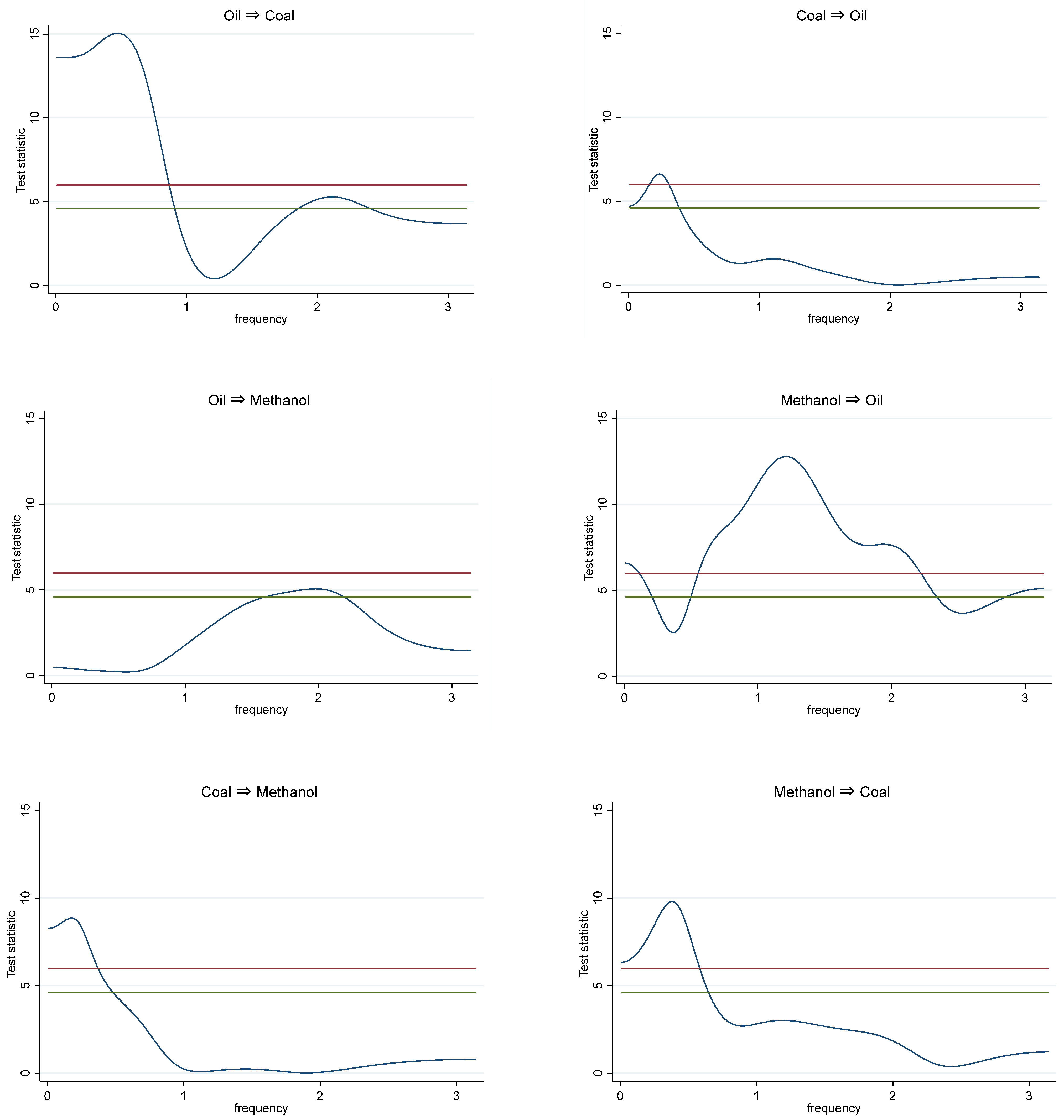
3.2. Granger Causality

We now turn to the Granger causality tests to uncover the direction of information flow in our tri-variate system. We carried out the frequency domain GC tests on our tri-variate system, testing GC between each pair of variables conditioned on the third variable. The results are plotted in Figure 3. In each diagram, the red and green horizontal lines represent the 5% and 10% critical values, respectively. When the test statistic curve lies above the horizontal lines, the null hypothesis of the Granger non-causality is rejected for that specific frequency. GC is evident from the oil price to coal price for all frequencies smaller than 0.87 at 5% significance and between frequencies of 1.86 and 2.39 at 10% significance. These frequencies and the corresponding wavelengths imply GC from 7.2 months (≈2π/ω) onwards and between 2.6 and 3.3 months. GC was also detected from the coal price to oil price in all frequencies smaller than around 0.38 (~16.5 months onwards). It is worth noting that the long-run causality (i.e., GC at or near zero frequency) was expected in our system as cointegration was found amongst the variables.

On the relationship between oil and methanol prices, we found GC from the oil price to methanol price at frequencies between 1.61 and 2.18 (wavelength between 3 and 4 months), implying that a short-term component of the methanol price is significantly affected by oil price. On the other hand, we found GC running from the methanol price to oil price at all frequencies other than 0.21–0.49 and 2.34–2.85, meaning that information of the methanol price can be used to improve forecasts of Chinese oil import price in both the short- and long-term. Finally, bi-directional GC was found between the coal price and methanol price in a similar range of lower frequencies, pointing to causalities only in the longer term (>10 months).

As a supplement to the frequency domain GC tests, time domain GC tests were performed, and the Wald test results are presented in

Table 4. Time domain Granger causality results.

Causal Direction	Test Statistic	p-Value
Mt→ Ot	28.08	0.000
Ct→ Ot	9.84	0.132
Ot→ Mt	6.50	0.370
Ct→ Mt	12.65	0.049
Mt→ Ct	14.00	0.030
Ot→ Ct	19.80	0.003

H₀: no Granger causality.

. Using a significance level of 10%, we observed unilateral causality from the oil price to coal price, and from the methanol price to oil price. Bi-directional causality was found between the coal and methanol pair. Considering the frequency domain and time domain GC results side-by-side, we found that the frequency domain tests discovered causal directions that were not picked up by the time domain tests. This is primarily due to the ability of frequency domain tests to offer deeper insights with regards to the dynamics of the causality across different frequencies. This highlights the advantage of the frequency domain GC tests in our empirical analysis.

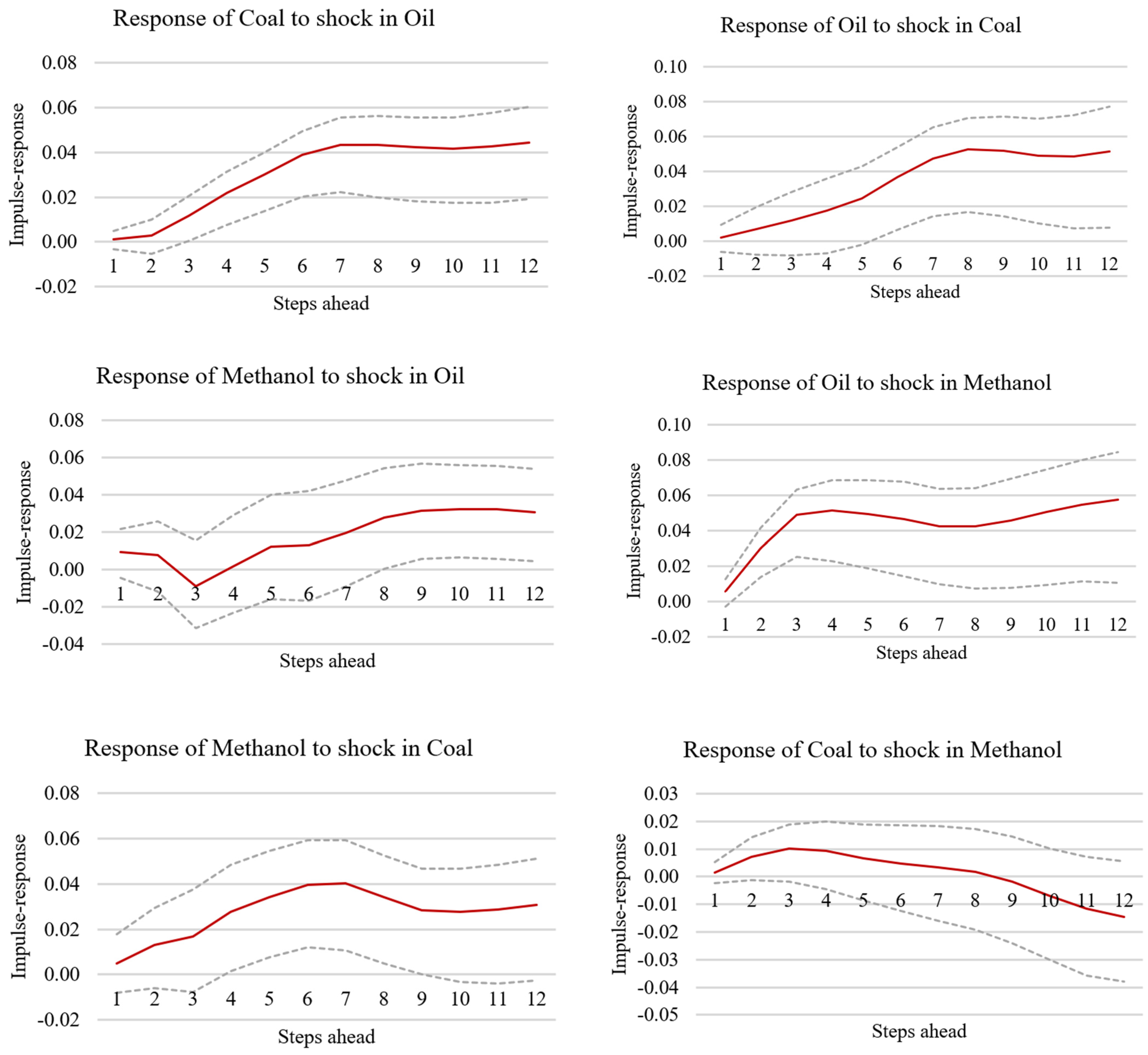
3.3. Generalized Impulse-Response Functions

To further visualize the relationships among the price series, we computed the generalized impulse response functions (GIRF) proposed by Pesaran and Shin [43]. Considering that three out of four indicators in Section 3.1 suggest a cointegration rank of 1, our computations proceeded with a VECM of rank 1. The GIRFs are displayed in Figure 4. The functions (in solid line) described the response of a variable to a one standard deviation shock in another variable over a 12-month horizon. Bootstrapped 90% confidence intervals are shown by dotted lines.

Following a shock in the price of oil, the price of coal responded statistically significantly with a three-month lag, and the magnitude of the response continued to increase before stabilizing from seven months onwards. Reversing the direction, a shock in the coal price induced a statistically significant positive response in the oil price from six months onwards. A shock in the methanol price lead to a positive response in the oil price, and the reverse is also true, albeit with an eight-month lag. These results indicate a reasonable degree of connectedness between the two prices, which is unsurprising due to the ability to substitute between methanol and gasoline.

While a shock in the methanol price did not trigger any statistically significant response in the coal price, shocks in the coal price were transmitted to the methanol price, and the positive response was statistically significant in four months after the shock and then leveled off and became insignificant from nine months onwards. The connection between coal and methanol prices were expected given the importance of coal as a major feedstock in methanol production. Consonant with the GC results, the price of coal appears to receive information from the oil price, while helping predict the methanol price.

4. Policy Implications and Future Research

Here we pause and reflect on the relevance of our results to the domestic energy policy in China. Building on discussions in the introduction, and conditional on our econometric results illustrating that China’s coal prices are impacted by methanol and international oil prices, we briefly consider the wider consequences to power markets. The concern implied by our results is that it may become possible that Chinese electric power prices for residential consumers, and industrial users, may be increasingly impacted by external market pressures, e.g., that oil prices could in fact manifest in cost pressure for electric power producers. While we do not prove this to be so through any modeling, nor do we offer any thought on how such relations ought to be handled, we nonetheless feel that our results, combined with a cursory examination of historic electric prices, point towards the need for an additional investigation and offer a direction for future research.

From Figure 5 we see that residential prices for electricity have been largely stable since 2006, with notional variation around a ‘benchmark’ price of around 0.525 RMB/kWh. A more striking feature, however, is the change, and subsequent reversal, in the price trend for industrial consumers. From 2002 to 2014, industrial prices for electricity saw a persistent and close to linear increase from about 0.525 RMB/kWh up to 0.8 RMB/kWh. Towards the end of 2014, approximately, the trend altered and prices stabilized for a while before going into a heavy decline from the end of 2017. Referring to Figure 2, we can observe that these timings loosely coincide with major coal and oil price movements. More specifically, towards the end of 2014, oil prices fell from 5000 RMB/t to around 2500 RMB/t, and have net reversed to pre-2014 levels. As for coal, in the third quarter of 2016, prices rose quickly away from 400 RMB/t and stabilized at around 600 RMB/t where it has remained until the end of the sample period.

We do not seek here to attribute any causal association from the above-mentioned movements in coal/oil prices to city average electricity prices, yet suspect their relation may be more than pure coincidence. Future research might seek to explore this issue more directly. In doing so, it would also seem relevant to question the salience of the price wedge between industrial and residential electric prices. Price variability was clearly skewed towards industrial power users, which may be justifiable. Nonetheless, in the final years of the sample, this manifests in double-digit percentage changes in price, which are not matched in residential prices. One concern here would be that the prevailing cost conditions for power generation may be benefited by the advances in energy technologies. If the electricity cost reductions derive from changes in production cost, are these benefits being passed on to the consumers in a fair or appropriate manner? Any proper answer to this question would require thorough analysis, but since these questions sit outside of the purpose of this paper, we leave this as an avenue for future research.

5. Conclusions

In this paper, we examined the relationships among crude oil, methanol and coal prices in China. The analysis was motivated by the concern that, with coal-to-liquid technologies becoming increasingly commercially viable, coal prices in China may be interconnected with other fuel prices, specifically oil and methanol. This was examined with a combination of cointegration analyses and two types of Granger causality tests (one in the time domain, another in the frequency domain). The price formation of coal is observed to be dependent on oil prices and methanol prices. Cointegration is found among the three prices and the generalized impulse response functions indicate that shocks in the oil price can stimulate a positive response in the coal price. Taking the two types of GC results together, we found clear evidence of GC running from oil and methanol prices to the coal price; thus, exemplifying their importance in explaining and predicting the price of coal in China. Beyond extending our understanding on the coal price formation, our results also emphasize the strong connection between methanol prices and both oil and coal prices.

The frequency domain-based causality analysis provided additional insights on the causal relations in the system that could have been missed had we performed only GC tests in the time domain. In all cases where GC exists (i.e., all cases except from oil to methanol), long-run causality is also detected. Both GIRF and frequency domain GC results indicate that methanol and coal prices are rather slow in responding to shocks in the oil price, while the oil price reacts more quickly to shocks in the methanol price. This may reflect the differences between the markets in terms of maturity and liquidity.

We can reconcile our empirical findings with economic theory given the substitutability between coal-based methanol and gasoline in China. When the price of crude oil rises, it leads to an upward pressure on the price of gasoline and, hence, creating an incentive to substitute gasoline for methanol. Other things being equal, the demand and price of methanol will tend to go up. The rise in price and the need to produce extra methanol will in turn raise the demand for the feedstock, which is coal in this case, lifting the price of coal as a result. Strong growth of the Chinese economy in recent decades and the country’s dominating scale in demand and supply of coal have shifted the geographical balance of the world coal market. The empirical linkage found between Chinese coal and oil prices in this paper may eventually have broader implications on the movement of other coal prices in the world. Causality in the opposite direction is equally plausible according to the economic theory, and our frequency domain GC results show that shocks originating from coal affect both methanol and oil.

References

1. IEA. World Energy Outlook 2019; International Energy Agency: Paris, France, 2019. [Google Scholar]
2. Yang, C.J.; Xuan, C.W.; Jackson, R.B. China’s coal price disturbances: Observations, explanations, and implications for global energy economies. Energy Policy 2012, 51, 720–727. [Google Scholar] [CrossRef]
3. Meng, T.; Huo, X.F. Study on the factors affecting international coal price. Price Theory Pract. 2008, 5, 55–56. (In Chinese) [Google Scholar]
4. Cao, C.F. Empirical study on changing tendency and influencing factors of coal price in China. Master’s Thesis, Xi’an University of Science and Technology, Xi’an, China, 2010. (In Chinese). [Google Scholar]
5. Hao, X.; Song, M.; Feng, Y.; Zhang, W. De-Capacity Policy Effect on China’s Coal Industry. Energies 2019, 12, 2331. [Google Scholar] [CrossRef] [Green Version]
6. BP. World Energy Statistics 2019; BP: London, UK, 2019. [Google Scholar]
7. Warell, L. Market Integration in the International Coal Industry: A Cointegration Approach. Energy J. 2006, 27, 99–118. [Google Scholar] [CrossRef] [Green Version]
8. Li, R.; Joyeux, R.; Ripple, R.D. International steam coal market integration. Energy J. 2010, 31, 181–202. [Google Scholar] [CrossRef] [Green Version]
9. IEA. Medium-Term Coal Market Report 2016; International Energy Agency: Paris, France, 2016. [Google Scholar]
10. Park, C.; Chung, M.; Lee, S. The effects of oil price on regional economies with different production structures: A case study from Korea using a structural VAR model. Energy Policy 2011, 39, 8185–8195. [Google Scholar] [CrossRef]
11. Masih, R.; Peters, S.; De Mello, L. Oil price volatility and stock price fluctuations in an emerging market: Evidence from South Korea. Energy Econ. 2011, 33, 975–986. [Google Scholar] [CrossRef]
12. He, Y.N.; Wang, S.Y.; Lai, K.K. Global economic activity and crude oil prices: A cointegration analysis. Energy Econ. 2011, 32, 868–876. [Google Scholar] [CrossRef]
13. Zhang, Y.J.; Wei, Y.M. The crude oil market and the gold market: Evidence for cointegration causality and price discovery. Resour. Policy 2010, 35, 168–177. [Google Scholar] [CrossRef]
14. Esmaeili, A.; Shokoohi, Z. Assessing the effect of oil price on world food prices: Application of principal component analysis. Energy Policy 2011, 39, 1022–1025. [Google Scholar] [CrossRef]
15. Nazlioglu, S.; Soytas, U. Oil price, agricultural commodity prices, and the dollar: A panel cointegration and causality analysis. Energy Econ. 2012, 34, 1098–1104. [Google Scholar] [CrossRef]
16. Zamani, N. The Relationship between Crude Oil and Coal Markets: A New Approach. Int. J. Energy Econ. Policy 2016, 6, 801–805. [Google Scholar]
17. Bachmeier, L.J.; Griffin, J.M. Testing for Market Integration Crude Oil, Coal, and Natural Gas. Energy J. 2006, 27, 55–72. [Google Scholar] [CrossRef]
18. He, W.; Lu, X.S. Study on the relationship between coal and crude oil prices. Energy Tech. Manag. 2011, 5, 16–27. (In Chinese) [Google Scholar]
19. Mjelde, J.W.; Bessler, D.A. Market integration among electricity markets and their major fuel source markets. Energy Econ. 2009, 31, 482–491. [Google Scholar] [CrossRef]
20. Jiao, J.L.; Fan, Y.; Wei, Y.M. The structural break and elasticity of coal demand in China: Empirical findings from 1980–2006. Int. J. Glob. Energy Issues 2009, 31, 331–344. [Google Scholar] [CrossRef]
21. Joets, M.; Mignon, V. On the link between forward energy prices: A nonlinear panel cointegration approach. Energy Econ. 2012, 34, 1170–1175. [Google Scholar] [CrossRef] [Green Version]
22. Mohammadi, H. Electricity prices and fuel costs: Long-run relations and short-run dynamics. Energy Econ. 2009, 31, 503–509. [Google Scholar] [CrossRef]
23. Mohammadi, H. Long-run relations and short-run dynamics among coal, natural gas and oil prices. Appl. Econ. 2011, 43, 129–137. [Google Scholar] [CrossRef]
24. Huang, H.; Fletcher, J.J.; Sun, Q. Modeling the impact of coal-to-liquids technologies on China’s energy markets. J. Chin. Econ. Foreign Trade Stud. 2008, 1, 162–177. [Google Scholar] [CrossRef]
25. Breitung, J.; Candelon, B. Testing for short- and long-run causality: A frequency-domain approach. J. Econom. 2006, 132, 363–378. [Google Scholar] [CrossRef]
26. Elliott, G.; Rothenberg, T.J.; Stock, J.H. Efficient tests for an autoregressive unit root. Econometrica 1996, 64, 813–836. [Google Scholar] [CrossRef] [Green Version]
27. Perron, P.; Qu, Z. A simple modification to improve the finite sample properties of Ng and Perron’s unit root tests. Econ. Lett. 2007, 94, 12–19. [Google Scholar] [CrossRef]
28. Kwiatkowski, D.; Phillips, P.C.B.; Schmidt, P.; Shin, Y. Testing the null of stationarity against the alternative of a unit root: How sure are we that economic time series have a unit root? J. Econom. 1992, 54, 159–178. [Google Scholar] [CrossRef]
29. Johansen, S. Likelihood-Based Inference in Cointegrated Vector Autoregressive Models; Oxford University Press: Oxford, UK, 1995. [Google Scholar]
30. Gonzalo, J.; Pitarakis, J.-Y. Specification via model selection in vector error correction models. Econ. Lett. 1998, 60, 321–328. [Google Scholar] [CrossRef] [Green Version]
31. Aznar, A.; Salvador, M. Selecting the rank of the cointegration space and the form of the intercept using an information criterion. Econom. Theory 2002, 18, 926–947. [Google Scholar] [CrossRef]
32. Toda, H.Y.; Yamamoto, T. Statistical inference in vector autoregressions with possibly integrated processes. J. Econom. 1995, 66, 225–250. [Google Scholar] [CrossRef]
33. Dolado, J.J.; Lutkepohl, H. Making Wald tests work for cointegrated VAR systems. Econom. Rev. 1996, 15, 369–386. [Google Scholar] [CrossRef]
34. Geweke, J. Measurement of linear dependence and feedback between multiple time series. J. Am. Stat. Assoc. 1982, 77, 304–313. [Google Scholar] [CrossRef]
35. Hosoya, Y. The decomposition and measurement of interdependency between second-order stationary process. Probab. Theory Relat. Fields 1991, 88, 429–444. [Google Scholar] [CrossRef]
36. Ciner, C. Oil and stock returns: Frequency domain evidence . J. Int. Financ. Mark. Inst. Money 2013, 23, 1–11. [Google Scholar] [CrossRef]
37. Wei, Y.; Guo, X. An empirical analysis of the relationship between oil prices and the Chinese macro-economy. Energy Econ. 2016, 56, 88–100. [Google Scholar] [CrossRef]
38. Ahmed, M.; Azam, M. Causal nexus between energy consumption and economic growth for high, middle and low income countries using frequency domain analysis. Renew. Sustain. Energy Rev. 2016, 60, 653–678. [Google Scholar] [CrossRef]
39. Batten, J.A.; Ciner, C.; Lucey, B.M. The dynamic linkages between crude oil and natural gas markets. Energy Econ. 2017, 62, 155–170. [Google Scholar] [CrossRef]
40. Aydin, M. Natural gas consumption and economic growth nexus for top 10 natural Gas–Consuming countries: A granger causality analysis in the frequency domain. Energy 2018, 165, 179–186. [Google Scholar] [CrossRef]
41. Gorus, M.S.; Aydin, M. The relationship between energy consumption, economic growth, and CO2 emission in MENA countries: Causality analysis in the frequency domain. Energy 2019, 168, 815–822. [Google Scholar] [CrossRef]
42. Lemmens, A.; Croux, C.; Dekimpe, M.G. Measuring and testing Granger causality over the spectrum: An application to European production expectation surveys. Int. J. Forecast. 2008, 24, 414–431. [Google Scholar] [CrossRef]
43. Pesaran, M.H.; Shin, Y. Generalized impulse response analysis in linear multivariate models. Econ. Lett. 1998, 58, 17–29. [Google Scholar] [CrossRef]
Figure 1. Coal production and consumption of China (2010–2019). Data source: National Bureau of Statistics of China.
Energies 14 03752 g001
Figure 2. China coal and crude oil prices (January 2010–December 2019). Oil import price is shown on the primary axis; coal price is shown on the secondary axis. Data source: Datastream and CCTD.
Energies 14 03752 g002
Figure 3. Frequency domain Granger causality tests. The red and green horizontal lines represent the 5% and 10% critical values, respectively. When the blue line sits above the critical values, we may conclude the existence of causality at the frequency level identified along the x-axis.
Energies 14 03752 g003
Figure 4. Generalized impulse-response functions. Dotted lines show 90% confidence bounds. When zero lies within the dashed lines (the 90% confidence interval), the response of the variable to a shock from another is considered statistically equal to zero and insignificant.
Energies 14 03752 g004
Figure 5. A total of 36 city average electricity prices in China. Prices are in RMB/kWh. Data source: CEIC database. Data reported cover the period January 2010–December 2019.
Energies 14 03752 g005