3D Modeling of the Thermal Transfer through Precast Buildings Envelopes

Abstract

In this paper, a finite-element-based model is being introduced and developed, using the Cast3m (CEA, Paris, France) simulation tool, to evaluate the thermo-mechanical behavior of a small-scale test bed. In fact, many studies on thermal behavior of cavities have been carried out in literature. However, none of them took into account the co-existence of all thermal phenomena (conduction, convection, internal/external radiation). The work presented in this paper presents a thermo-mechanical model, which aims to combine, in a holistic way, these phenomena. An experimental validation of the thermal model has been first carried out using an infrared camera and DS18B20 (Maxim Integrated Products, Dallas, TX, USA) numerical sensors. Results are reported and show the accuracy of the proposed model since both numerical and experimental values of heat transmittance fit together. The main objective is to evaluate heat losses through the walls, by means of heat transmittance calculation, and proposing new functional materials that will help in energy harvesting, as a perspective of this work. As for the mechanical study, it was meant to investigate the distribution of the mechanical stress towards the building envelope submitted to its own weight. Results showed that the stress is uniformly distributed on the lateral walls of the structure as well as on the floor.

1. Introduction

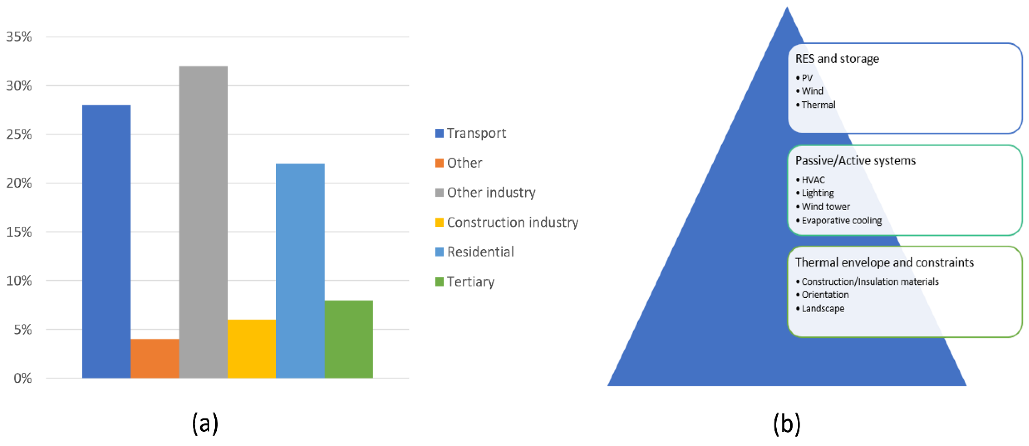
Worldwide, the construction and building sector is responsible for more than 40% of total energy consumption (see Figure 1a) and contributes one third of CO₂ emissions [1]. In Morocco, consumption represents about 25%, from which 18% concerns residential buildings while the rest is devoted to the tertiary sector [2].

This expenditure will escalate even more in the coming years given an increasing rate of population increase, as well as the still-improving standards of living [3]. This will not only lead to an increase in the construction rate and in the use of household equipment (e.g., HVAC), which increase electricity consumption, but also to the increase of harmful gas emissions. In order to face the climate change facing the world, reducing energy consumption is becoming an obligation more than a luxurious choice of living. Different countries have adopted laws and construction regulations in order to rationalize construction behavior and register the building sector through energetic sobriety while emphasizing on the comfort of occupants. Indeed, seventy-three countries have their own codes while eight are in the development process. Among these seventy-three, we can find four with voluntary residential codes, twelve with voluntary tertiary codes, fifty-one with imperative tertiary codes and forty-one with obligatory residential codes [4].

Thermal regulation represents a basic document for energy optimization in a building’s envelope at the design and conception phases. The appropriate approaches have been then developed to fit each zone according to its corresponding meteorological data [5]. In fact, one of the most efficient approaches to ensure energy efficiency in buildings is to analyze and study interfaces between all involved aggregated components (see Figure 1b) [6]: (i) much attention should be paid to the building’s construction materials (envelope and internal partitions) and its properties (orientation, landscape, design, internal distribution of the components, etc.), (ii) integration of active/passive systems in order to boost audible, visual and thermal comfort by integrating ICT technologies and concepts (e.g., Internet of Things, Big Data, forecast and prediction analytics) for data acquisition and control [7], and (iii) efficient incorporation of renewable energy technologies (e.g., solar panels, wind turbines) [8] and energy storage [9,10] devises (e.g., batteries, hydrogen).

The main idea behind this work is to focus on the building’s envelope by investigating the impact of thermo-mechanical aspects on its behavior. In literature, many researchers have carried out lots of work on thermal analyses of building as a means of ensuring thermal comfort. Candau and Piar [11] tracked indoor temperature of a building in response to externally imposed excitations. A comparative study between simulation and experimentation has been held, basing their analysis on, respectively, model identification and spectral analysis. Gargari et al. [12] presented in their work a ‘public housing’ building type simulation to evaluate energy savings generated by the change of insulation materials for external walls while adopting a green roof solution. Results showed that for a building with insulation that responds to restrictive energy regulation, moderate benefits are received from a green roof’s integration. Houda et al. [13] worked on improving the evaluation method of thermal comfort in office buildings through the arid zones with dry and hot climates, by the analysis of the external intervening parameters. It was shown that predictive comfort and perceived comfort are different, since the first can be calculated based on bioclimatic parameters; as for the second, it varies according to occupants.

Not only that, but other researchers have also investigated cavities with various geometries and a variety of construction materials. For instance, Markatos and Perideous [14] refined a calculation method essentially intended to procure solutions of heat transfer, turbulent flow and buoyancy-driven laminar flow in a square cavity with differentially heated side walls. They also took into consideration a refined mesh for fairly high Rayleigh numbers. The outcomes of their research mainly concern rectangular cavities with Rayleigh numbers going up to 10⁶, a Prandtl number of 0.71 and an aspect ratio of 1. Nonetheless, the method is considered to be more general and can be applied to any kind of geometry. Another interesting work has been performed by Cordoba et al. [15]. In this, the authors conducted a numerical study on a laminar, steady, incompressible, free convection with surface radiation in a two-dimensional open cavity. A heating source was imposed on the wall in parallel to the opening, while the rest of the walls were considered adiabatic. The governing equations of, respectively, energy, mass and momentum were resolved based on the usage of a finite volume approach, which was implemented in FORTRAN. Their study revolved around heat transfer characteristics, the orientation of the structure, and the influence of surface radiation on the fluid flow. Reported results showed that the heat transfer decreases when decreasing the cavity tilt angle for all used values of Rayleigh number and emissivity. They also mentioned that, at a certain tilt angle value, thermal radiation exchange between walls is much more significant. De Vahl [16] investigated the bi-dimensional circulation of air in an enclosed square cavity. Desirable movement was generated using a gradient of temperature imposed at both left and right walls as boundary conditions. Accordingly, De Vahl was able to prove that, in terms of vorticity transport and energy equations for Rayleigh numbers, up to 2 × 10⁻⁵, can converge. Additionally, he also reported the impact of the Prandtl number, which can play the role of a stabilizing factor, especially if it ranges from 10⁻¹ to 10³. Karatas and Derbently [17], in their study, have considered conjugated radiation and natural convection in a rectangular-shaped closed cavity with only one active vertical wall. The cooled surface is made of aluminum and plastic for the rest of the structure. However, since all walls are painted in white, the emissivity is considered to be constant.

Other research work focused on the influence of the aspect ratio on the Nusselt number and hence on the heat transfer with respect to the height of the cavity. For example, Yousaf and Usman [18] presented, in their work, an algorithmic study on a natural convection in two-dimensional square cavity with the presence of sinusoidal roughness elements, which are located simultaneously on hot and cold walls. To solve momentum and energy equations, various Rayleigh numbers, varying between 10³ and 10⁶, were used for a Newtonian fluid with a Prandtl number of 1. Results showed that the presence of these elements has an impact on the hydrodynamic and thermal behavior of the fluid in the cavity. Khatamifar et al. [19] presented numerical simulation results related to combined heat transfer and natural convection flow in a gradually heated square cavity for a large scope of the Rayleigh number (10⁵–10⁹). In fact, simulations were carried out using the finite volume method following three dimensionless partition thicknesses and positions. Results showed that the Nusselt number increases with the Rayleigh number but decreases with the thickness. Pandey et al., in their paper [20], presented a review of numerical and experimental research works linked to natural convection in enclosures with/out the presence of internal bodies. These latter were taken under different shapes in order to figure out their impact on buoyancy driven-flow among enclosures. The used methods mainly cover spectral element method, finite element approaches, Latice Boltzmann method (LBM), finite volume method and so on. Their paper also discussed the effect of multiple parameters, such as Rayleigh, Grashof, and Prandtl numbers, in order to make the optimal choice of design parameters according to the desired system requirements. Ouakarrouch et al. [21] presented a simulation englobing the conduction heat transfer and natural convection as well as radiative heat through two kinds of alveolar walls used in a recent building’s construction (3- and 6-hole numbers). Results showed that heat transfer is increased once radiative transfer is considered into calculations. Further, it was proved that conductive transfer accounts for almost the half of the heat flux in the block of 20 incorporating a thermally conducting vertical partition.

In most of the research work, and to the best of our knowledge, researchers mainly emphasize characterizing the thermal behaviors of cavities with different shapes. These latter are either heated using sun rays or a simple heating source so that an active wall is always present. They almost never take into account the co-existence of all thermal phenomena (natural convection, conduction, internal/external radiation) to study the thermal behavior of regular cavities. In the work presented in this paper, we shed more light on the thermal characterization of the envelope of a chosen structure using a combination between radiation, conduction among the different materials, and natural convection in a rectangular cavity clogged with air. Not only that, but we also conduct a mechanical study to evaluate stress distribution on the walls of a structure subjected to its own weight.

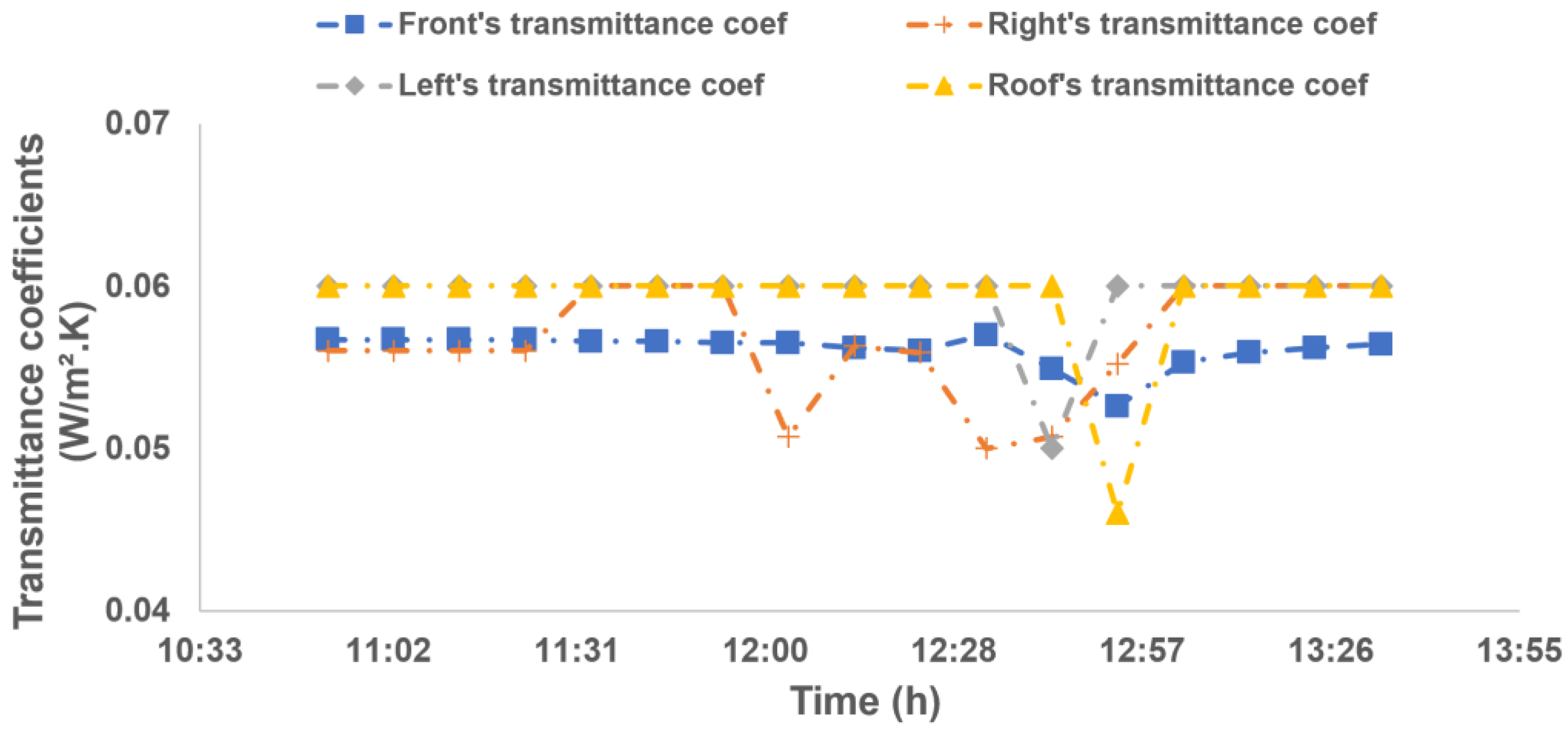
The main objective is to carry out a transient thermo-mechanical characterization of buildings’ envelopes. In fact, we are aiming to evaluate heat losses through the walls and especially through potential thermal bridge areas, by means of calculating transmittance coefficients. Once the behavior is known and the simulation models are fitted by means of experimentations in real sitting scenarios, we will be able to introduce (as perspective to this work) new functional materials in order to decrease heat losses and to contribute to energy harvesting.

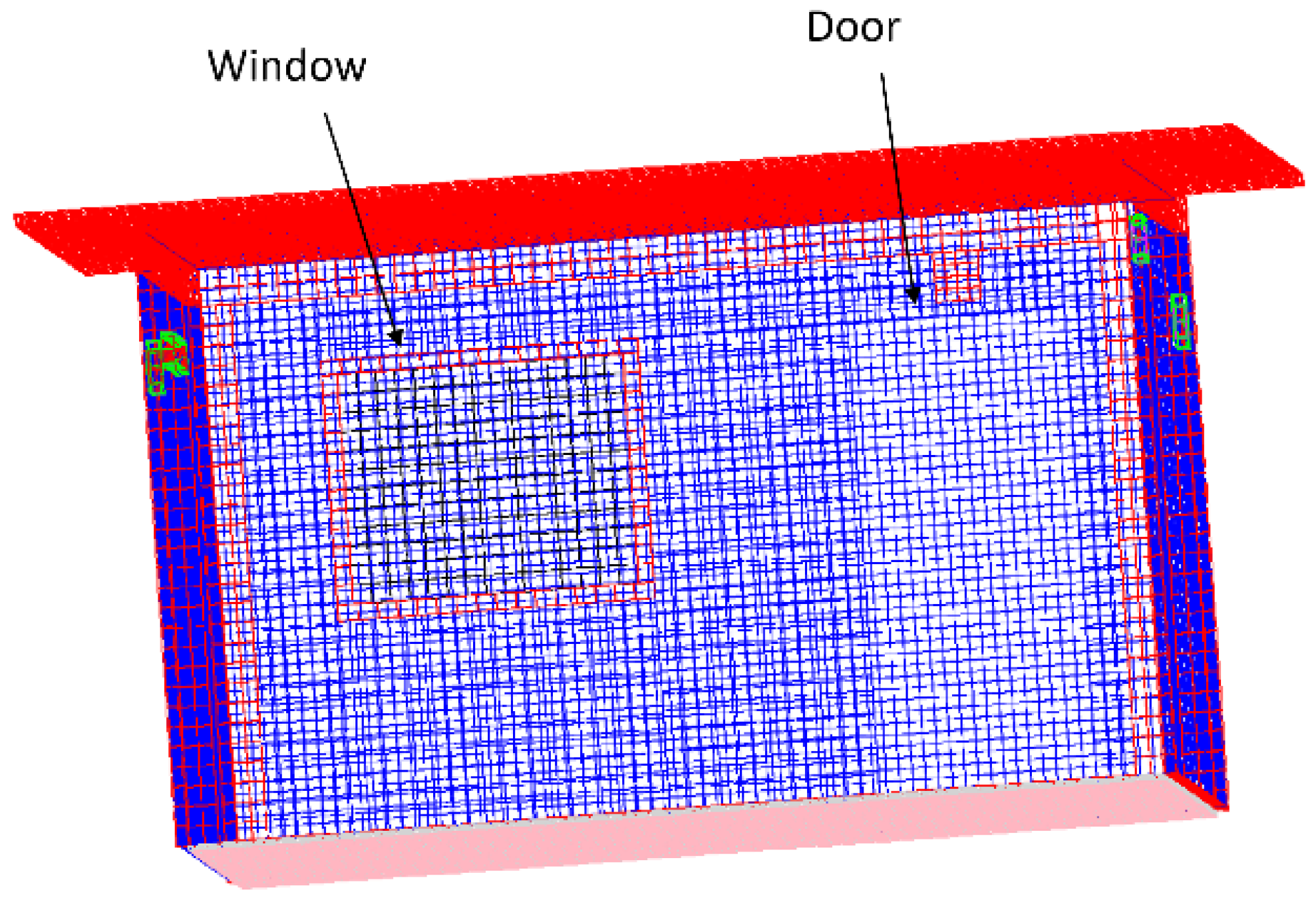
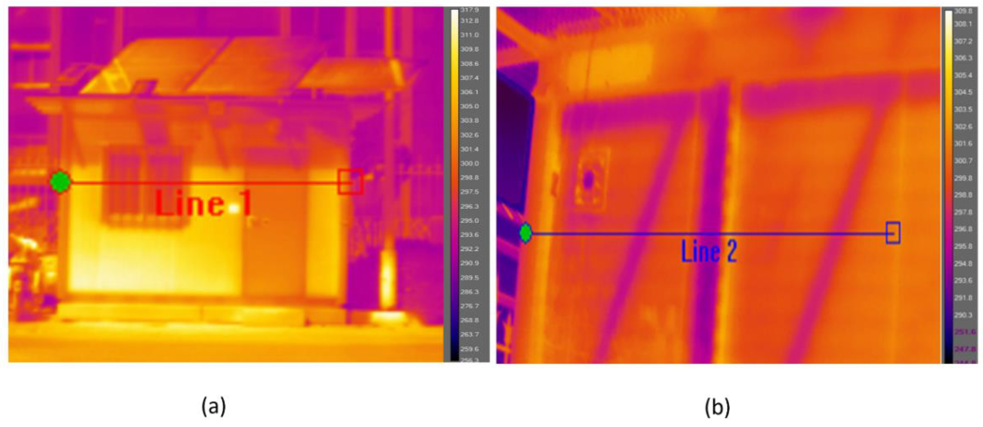
A small-scale building, called EEBLAB (Touax Maroc, Mohammedia, Morocco) (energy efficient building laboratory), is used as a testbed in order to conduct experimental and simulation evaluations. Its structure is essentially made of galvanized steel for the external walls, roof and flooring base. Expanded polyurethane is injected into the external walls as a means of insulation. Two types of internal insulation are used: chipboard for the floor and an air gap and plaster boards for the roof. Thermal sensors are placed in different areas on the surfaces of the walls in order to obtain real-time temperature values, which are used to evaluate thermal transmittance coefficients. It is also worth to note that some sensors are placed in areas where thermal bridges are expected to appear. These areas were distinguished using a thermal camera [22] (thermography analysis). Based on experimental results, a finite-element-based numerical model was developed. Simulations were directed and the main outputs are presented to show the accuracy and the performance of the developed mechanical and thermal models.

The leading grants of this work compared to our previous published paper [23] are threefold:

• Extensive experiments have been conducted using thermography analysis to detect thermal bridge placement among the EEBLAB.
• A transient numerical model is proposed for buildings’ thermal characterization, taking into account its dynamic behavior.
• A mechanical numerical model is presented to evaluate the distribution of mechanical stress towards buildings’ envelopes in response to the effect of their own weights.

The remainder of this paper is structured as follows. Section 2 presents an overview of the theoretical backgrounds allowing the creation of both thermal and mechanical models. In Section 3, we introduce the materials and methods, including numerical and experimental set-ups, used to develop and validate the numerical models. Results and discussion are presented in Section 4, where a mesh sensibility study is also presented. Section 5 concludes the paper and provides some perspectives on this work.

2. Theoretical Background

2.1. Thermal Model Equations

The performed thermal model includes conductivity within the materials, natural convection inside and outside the structure as well as both self-surface radiation and external radiation. The thermal transient problem in a certain domain Ω is mainly governed by the heat equation (Equation (1)) and Fourier‘s law [24] (Equation (2)). This latter describes the transmission caused by the difference in the temperature between two regions of a medium in physical contact; where $\rho$ is the density (kg/m³), C_p is the specific heat capacity (J/kg·K), q is the flux density (W/m²), S is the surface of the medium (m²), f is a function which includes all thermal loading sources, k is the conductivity (W/m·K), ∆T is the temperature variation, and n is the normal vector to the surface:

$$\rho C_p\frac{\partial T}{\partial t}+div\left(q\right)=f$$

(1)

$$Q=-k\frac{dT}{dn}={\displaystyle \iint }k·\Delta T·ndS$$

(2)

To resolve this kind of problem, we usually proceed by using variation methods and the resulting matrix system to solve on the element Ωe is given in the following equations:

$$C·\dot{T}+K·T=Q$$

(3)

where:

$$C_{ij}=\underset{{\Omega }_e}{{\displaystyle \int }}\rho ·C_p·N_i·N_j dV$$

(4)

$$K_{ij}=\underset{{\Omega }_e}{{\displaystyle \int }}\lambda ·grad\left(N_i\right)·grad\left(N_j\right) dV-\underset{\partial {\Omega }_c^e}{{\displaystyle \int }}h·N_i·N_j·dS-\underset{{\Omega }_c^e}{{\displaystyle \int }}\epsilon ·\sigma ·\widetilde{T^3}·N_i·N_j·dS$$

(5)

$$Q_{ij}=\underset{{\Omega }_e}{{\displaystyle \int }}f{N}_i dV-\underset{\partial {\Omega }_c^e}{{\displaystyle \int }}h·T_{ac}·N_i·dS-\underset{{\Omega }_c^e}{{\displaystyle \int }}\epsilon ·\sigma ·\widetilde{T^3}{T}_{ac}·N_i·dS-\underset{\partial {\Omega }_Q^e}{{\displaystyle \int }}{q}_0·N_i·dS$$

(6)

C, K and Q are respectively the capacity (J/kg·K), conductivity (W/m·K) and heat flux (W) matrixes.

The term convection refers to the heat transmission occurring between a certain surface and a fluid in motion when they are at different temperatures. This kind of transfer is usually divided into two categories depending on the nature of the flow. The first one concerns natural convection. It occurs mainly when the flow is induced by a difference in density, which varies with the temperature in the fluid. The second one is forced convection, which occurs when the flow is generated by external means, such as a fan or atmospheric winds.

The calculation of the heat flux, which is induced by natural convection, is estimated in two steps. First, we estimate the non-dimensional numbers of Grashof and Prandtl:

$$Gr=\frac{\beta g\Delta T{L_c}^3{\rho }^2}{{\mu }^2}$$

(7)

where β is the thermal expansion (K⁻¹), g is the gravity (m/s²), L_c is the characteristic length (m), $\rho$ is the density (kg/m³) and μ is the dynamic viscosity (Pa·s).

Following the Grashof number, the correlations in

Table 1. Correlations for the calculus of Nusselt number [25].

Geometry	Gr × Pr	$\mathit{\gamma }$	M
Vertical plate	104–109	0.59	1/4
	109–1013	0.021	2/5
Horizontal tube	104–2.12 × 107	0.53	0.25
	2.12 × 107–1012	0.13	0.33

allow calculating the Nusselt number as mentioned in Equation (8).

$$Nu=\gamma {\left(Gr·Pr\right)}^m$$

(8)

Then the heat transfer coefficient is computed by Equation (9):

$$h=\frac{\overline{Nu} L_c}{k}$$

(9)

The expression of the heat flux (W) is expressed following Equation (10), where T_a is the ambiance (internal or external) temperature (K), T is the temperature of the wall (K), and S represents the area of the wall (m²).

$$Q=h \left(T_a-T\right)S$$

(10)

In the formulation of the finite element problem adopted in our study, convection is accounted for by adding a convection matrix H, representing the coefficient h (W/m² K), to the conductivity matrix, and the addition of a term Q_c, representing the term h × T_a, to the second member.

$$C·\dot{T}+\left(k+H\right)·T=Q+Q_c$$

(11)

On the other hand, Stefan-Boltzmann’s law translates the radiant thermal transfer, where ε is the emissivity of the used material and φ is the heat flux density (W/m²).

$$Q=\epsilon \sigma S\left({T_a}^4 -T^4\right)$$

(12)

The condition at the radiation limits is thus considered as an equivalent condition of convection with a nonlinear convective exchange coefficient h = ε·S·T³. This factor can be extracted by factorizing by the term (T_a − T) in Equation (12).

$$\left(T_a^4-T^4\right)=\left(T_a-T\right)\left(T^3+T^2{T}_a+T{T}_a^2+T_a^3\right)$$

(13)

In addition, thermal transmittance coefficients are estimated on walls, floors, roofs and windows as follows:

• Considering a wall separating two different atmospheres, the total thermal resistance is the set of all the layers of materials or air that constitute the wall, in addition to surface-exchange resistances (resulting from the phenomenon of convection) (see Figure 2a). From this resistance, we can obtain the heat transfer coefficient, which represents the amount of heat transmitted through this wall in steady state, per unit time, per unit area and temperature difference of one-degree Kelvin. In other words, this transmittance coefficient represents the opposite of the total thermal resistance of the wall and is given in W/m²·K.
• However, if the wall is made of several non-homogeneous materials, a very simplified calculation method can be used. It mainly consists of considering that the total thermal resistance is between upper and lower limits. These limits, for each case, could be computed by dividing the wall into different sections whose layers are homogeneous and then applying the normal rules of calculation.

According to Figure 2b, the transmittance coefficient (in W/m²·K) can be subdivided into two coefficients (upper and lower) and can be calculated as shown in Equations (14) and (15).

$$U_{up}=P_{as}{U}_{as}+P_{bs}{U}_{bs}+P_{cs}{U}_{cs}$$

(14)

$$U_{low}=P_1{U}_1+P_2{U}_2+P_3{U}_3$$

(15)

where, U_up is the upper limit of the transmission heat coefficient. U_low is the lower limit of the transmission heat coefficient. P_as, P_bs, P_cs, P₁, P₂ and P₃ are respectively the percentage of material constituting layer a_s, b_s, c_s, 1, 2 and 3.

The total heat transfer coefficient (U_T) is then expressed as follows:

$$U_T=\frac{U_{up}+U_{low}}{2U_{up}{U}_{low}}$$

(16)

In order to obtain more accuracy in terms of calculations, thermal bridges should be taken into account. They essentially designate the heat losses through the interfaces of constructive elements and must be added to the surface losses. They are largely divided into two categories. The first category represents structural thermal bridges, which are related to the techniques used for insulator placement as well as those of constructions in the frame of wood. The second category represents thermal bridges due to geometric constraints, which are linked to the shape of the envelope.

Broadly, the main thermal bridges of any kind of buildings are located at the articulations of the facades and floors, facades and roofs, facades and opening frames. If the walls are highly insulated, thermal bridges persist more than usual and, hence, thermal losses increase. Therefore, in the case of low-consumption buildings, such as small-scale structure we are considering in this study, having high thermal resistances could ensure low heat losses per junction. If these leakages are not treated, they will cause discomfort for occupants, increase energy expenses, and might cause a deterioration of materials as well.

Taking into account thermal bridges’ effect, the global thermal transmittance is given in Equation (17):

$$U_T=\frac{1}{{\displaystyle \sum }{R}_{layer}+{\displaystyle \sum }{R}_s}+\frac{{{\displaystyle \sum }}_i{\psi }_i{L}_i+{{\displaystyle \sum }}_j{\chi }_j}{S}$$

(17)

where ${\psi }_i{L}_i$ represents punctual thermal bridges, ${\chi }_j$ represents linear thermal bridges and S is the surface of the layer.

As with heat losses through the walls, thermal transmittance of the window needs to be considered. The EEBLAB window consists mainly of two parts: the aluminum frame and the glazing. For each of these parts, we must calculate the heat transfer coefficient. It should be noted that the outline of the glazing is affected by additional heat loss resulting from the combined effects of the frames, panels and spacers (constituting the linear thermal bridges). All of these elements make it possible to determine, by computing, the heat transfer coefficient of the window U_w [26].

$$U_w=\frac{S_g{U}_g+S_f{U}_f+P_g{\psi }_g}{S_g+A_f}$$

(18)

It is possible to generalize this formula, as shown in Equation (19), if we take into account the panel of the window or the ventilation grid. P_g is the visible perimeter of the glazing; S_g, S_f, S_p and S_vg are respectively the surfaces of the glazing, frame, panel and ventilation grid.

$$U_w=\frac{S_g{U}_g+S_f{U}_f+P_g{\psi }_g+S_{vg}{U}_{vg}+P_p{\psi }_p+S_p{U}_p}{S_g+S_f+S_{vg}+S_p}$$

(19)

The “building energy performance” regulation provides a simplified formula for evaluating the effectiveness of glazing and framing, while taking into account good airtightness [26]. The proportion varies depending on whether the glazing is more thermally efficient or the reverse.

If the transmittance coefficient of the glazing is less than the transmittance coefficient of the frame, the total transmittance coefficient of the window is given as in Equation (20):

$$U_w\left(\mathrm{W}/{\mathrm{m}}^2\mathrm{K}\right)=0.7U_g+0.3U_f+3{\psi }_g+\frac{{\displaystyle \sum }{S}_{vg} \left(U_{vg}-U_g\right)}{{\displaystyle \sum }{S}_w}$$

(20)

Otherwise,

$$U_w\left(\mathrm{W}/{\mathrm{m}}^2\mathrm{K}\right)=0.8U_g+0.2U_f+3{\psi }_v+\frac{{\displaystyle \sum }{S}_{vg} \left(U_{vg}-U_f\right)}{{\displaystyle \sum }{S}_w}$$

(21)

In the case of absence of ventilation grid and panel (which is our case), the formula becomes simple, as follows:

$$U_w\left(\mathrm{W}/{\mathrm{m}}^2\mathrm{K}\right)=0.7U_g+0.3U_f+3{\psi }_g$$

(22)

In other words, we consider 70% of glazing (since in most cases it is considered to be the most efficient [26], 30% of framing and 3 m of interlayer per m² of window.

2.2. Mechanical Model Equations

Considering a general problem of linear mechanics in small deformations, governed by the following equations.

• The equilibrium equation (Equation (23)), which illustrates the static or dynamic equilibrium of all external and internal forces of the studied system [27]:

$$div\left({\sigma }_d\right)=0$$

(23)

• The behavior law following three-dimensional Hook elasticity as shown in Equation (24).

$${\sigma }_d=\mathrm{C}:{\epsilon }_T$$

(24)

• The hypothesis of small deformations by assuming that the transformation between the initial equilibrium state and the current equilibrium state is infinitesimal [28], i.e.,

$${\epsilon }_T=\frac{1}{2}\left(\nabla U+\nabla U^T\right)$$

(25)

where ε_T, σ_d, U and C are respectively the total strain tensor (no unit), the stress tensor (N/m²), the displacement field (m) and the elasticity modulus tensor (Pa).

3. Materials and Methods

3.1. Numerical Set-Up

This section presents the geometry of our testbed building, together with parameters and tools used.

3.1.1. Geometry

The specimen considered in this study is one of the rectangular cavities, shown in Figure 3, based at our university. It is mainly deployed to investigate energy efficiency approaches for buildings.

This small scaled testbed has 12 m² of occupied surface and 30 m³ of volume.

Table 2. Dimensions of the EEBLAB and its components.

EEBLAB’s Dimensions (Height, Length, Width)	4 m × 3 m × 2.2 m
Window’s dimensions	1.2 m × 1 m
Door’s dimensions	0.85 m × 2.1 m

gives more information about its dimensions. It is essentially made from galvanized steel and expanded polyurethane injected into the walls for insulation purposes. The roof is made of a stratification of 3 layers (inside-out): plaster, air, galvanized steel. However, the floor is insulated using chipboard.

3.1.2. Structure Meshing

The same geometry of the EEBLAB was re-constructed in respect to the real dimensions (see Figure 4), so that precision and reliability of the model can be expected. The model is implemented on the cast3m tool, based on the finite element method, and using an Inspiron 157,000 gaming laptop with a processor of Intel^®Core™i7-7700HQ CPU@ 2.8 GHz, 2801 MHz, 4 cores and 8 logical processors (Dell Technologies, Round Rock, TX, USA). The assigned number of elements is 19,768 with about 41,030 nodes. Using the Cast3m tool, a density of 0.08 has been imposed in order to acquire the previously mentioned number of elements. The chosen type of meshing elements was cubic, since the geometry is regular and has a parallelepiped shape.

3.1.3. Parameters Identification

In order to perform simulations under Cast3m, complementary information about the construction and insulation materials parameters are needed, especially those related to thermal and mechanical types, as shown in

Table 3. Thermal properties of the construction and insulation materials of the EEBLab [29].

	Heat Capacity [J/kg·K]	Density [kg/m3]	Conductivity [W/m∙ K]
GS	470	7800	52
Chipboard	2100	170	0.042
PB	1300	25	0.022
Glass	800	2530	0.93
Al	900	2690	210
Pl	1000	40	0.024

GS (Galvanized steel), PB (Plasterboard), Al (Aluminium), Pl (Polyurethan).

and

Table 4. Mechanical properties of the construction and insulation materials of the EEBLAB [29].

Characteristics	Materials
	GSI	CB	PB	Al	Gl
Young Modulus (GPA)	200	12	2	68	69
Poisson ration	0.29	0.2	0.5	0.34	0.22
Density (kg/m3)	7800	7500	1250	2690	2530
Expansion coefficient (xE-06)	11	40	78	23	9

GS (Galvanized steel), CB (Chipboard), PB (Plasterboard), Al (Aluminium), Gl (Glazing).

.

3.1.4. Numerical Tools

In order to numerically compute the thermomechanical behavior of the EEBLAB’s envelope, the following procedures were considered. First, we start by the creation of a thermal solving procedure considering all the classical thermal phenomena (see Figure 5). Then, the second procedure is used to solve the mechanical equilibrium problem taking into account the own weight of the EEBLAB as the only force.

The main objective of the thermal procedure is to evaluate the transmitted flux among the EEBLAB’s walls in every single node. Hence, the calculation of the global heat transfer coefficient, including all thermal phenomena, is crucial. Figure 5 summarizes the steps of the computing procedures starting with the regeneration of the same EEBLAB’s geometry in respect to the real dimensions for more accurate results. Thermal parameters are also required to be declared as input data. For this, a manual thermometer was used to measure the needed information (ambient temperatures, walls’ temperatures) and exploit them to calculate the heat transfer coefficients using the classical correlations of Grashof and Nusselt (see Equation (8), Table 1).

It is worth to mention that the flow was considered as being laminar.

Table 5. Air characteristics depending on temperature.

Air Characteristics	Internal Ambiance	External Ambiance
T (Temperature)	297.8	291.5	K
G (Gravity)	9.81	9.81	N/kg
$\rho$ (Density)	1.187	1.217	kg·m−3
μ (Dynamic viscosity)	1.84 × 10−5	1.81 × 10−5	kg·m−1·s−1
ν (Cinematic viscosity)	1.54 × 10−5	1.46 × 10−5	m2·s−1
β (Coefficient of thermal expansion)	0.003358	0.003431	K−1
Cp (Specific heat)	1006	1005	J·kg−1·K−1
k (Conductivity)	0.026	0.0255	W·m−1·K−1

gives complementary information about air characteristics, which are needed for computing heat transfer coefficients.

(a)

Thermal Boundary and Interface Conditions:

In this subsection, thermal boundary and interface conditions (see Figure 6) are presented. Starting with boundary conditions (see Figure 6a), internal and external temperatures have been imposed on each facade of the walls as boundary conditions for convective heat transfer. As for considering the external radiative heat transfer, an infinite temperature of the value 500 K has been imposed. This latter also presents the initial temperature for numerical calculations. It is worth noting that internal radiative heat transfer has also been taken into account by calculating form factors.

For interface conditions, the external walls are made from different construction materials (multi-layers). Hence, it was supposed that during the calculation of heat transfer coefficients that layers in contact with each other have the same temperature at the contact interface. In other words, the contact resistance is neglected.

$$T_1\left(x_0,t\right)=T_2\left(x_0,t\right)$$

(26)

In addition, thermal conduction at the surface of the galvanized steel is equal to thermal conduction at the surface of the insulation layer. In other words, the interface between layers does not store energy (see Figure 6b).

$$-{\lambda }_1\frac{d{T}_1\left(x_0,t\right)}{dx}=-{\lambda }_2\frac{d{T}_2\left(x_0,t\right)}{dx}$$

(27)

(b)

Mechanical Boundary Conditions:

To launch the mechanical study of the EEBLAB using the Cast3m tool, we have supposed that the displacement following axes x, y and z are equal to zero. The building is subjected to its own weight (see Figure 7).

The EEBLab in both mechanical and thermal models is subjected to weather conditions of Sala El Jadida during the simulated periodof time, mainly in March 2019 (see Figure 8).

The resulted numerical data are extracted in nodes where the temperature sensors are placed on both external and internal walls. Figure 9 depicts the orthonormal reference, which allowed us to extract the exact coordinates of the location of the sensors.

It is worth to mention also that the characteristic length needed in the calculation of the Grashof number was taken as the width of the construction (LC = 4 m). The surface, which is needed to calculate the heat flux afterwards, is equal to 16 m² (LC²). This is because the EEBLAB’s walls have different surfaces, which may complicate the calculation process and takes more simulation time.

For the mechanical model, the main objective is to evaluate the structure resistance to external forces. However, it is important to first evaluate the mechanical resistance of the structure in response to its own weight. In this study, we mainly focused our interest on this part (see Figure 10). The code requires the geometry and all its mechanical characteristics. Functions and procedures are then integrated in order to evaluate the displacement and stress fields.

3.2. Experimental Set-Up

Experimental setup consists of using two essential devices (see Figure 11a). First, an infrared camera was deployed in order to observe temperature distribution among the studied surfaces and to identify thermal bridges’ placements as well. The camera was mainly focused towards the front and left facades, since they contain different materials and components (e.g., beams, door, window, etc.). The thermal analysis leads to areas where temperature sensors, specifically DS18B20 (Maxim Integrated Products, Dallas, TX, USA) should be placed (see Figure 11b).

These sensors provide temperature measurement in degrees Celsius on the order of 9 to 12 bits and are equipped with a user-defined alarm function. It communicates via a one-bus wire and contains a numerical resolution of 12 bits. This kind of sensor integrates all required functionalities to measure temperature: (i) analog sensor, (ii) analog/digital converter, and (iii) communication electronics and power supply [31]. For our case study, the sensors were linked to an embedded card. To perform the assembly, extra equipment was needed, such as a 4.7 K-Ohm resistance (code color yellow-violet-red), a circuit board and cables.

Depending on an already existing internet of things (IoT) framework, as mentioned in the work of NaitMalek et al. [32], the walls’ temperature data were regularly acquired during different periods of time. The data were collected and treated using an Intel^® Xeon^® CPU E5-2650 0 @ 2GHz computer (Dell Technologies, Round Rock, TX, USA); 64 Gb of RAM, a GPU of 43 Go-NVIDIA, an operating system of 64 bits and a 64 processor.

This collection of data allows analyzing and comparing both experimental and simulation results. Sensors were, symmetrically, placed on external as well as internal sides of the walls, so that the transmittance coefficients could be correctly evaluated. The obtained data were then transmitted, in real time, via Wi-Fi to our IoT platform for processing and storage.

4. Results and Discussions

In this part, a mesh model and grid independence checking study is presented. Besides, experimental and numerical results are given and confronted to each other in order to ascertain the finite element model developed on CAST3M.

4.1. Mesh Model and Grid Independence Checking

In this subsection, we present a meshing sensibility study. As was previously mentioned in Section 3.1.2, the chosen type of meshing element is cubic since the geometry of the EEBLab is a regular parallelepiped. According to the Cast3m programming, the size of the meshes, and hence the number of elements, can be easily changed by using the command ‘dens’. Focusing our interest on the mechanical study, we can notice (see

Table 6. Shear values according to meshing density.

Density of Meshing	SMXX (Shear Stress in Pa)
0.03
0.04
0.05
0.06
0.07
0.08
0.09

) that the shear stress value on the external walls slightly varies (from −6.58 × 10⁻⁶ Pa to 3.26 × 10⁻⁵ Pa) until reaching a ‘dens’ value of 0.06 (SMXX = 3.25 × 10⁻⁵ Pa). As known, reducing mesh sizing leads to increasing the number of elements, which might slow the simulation and certainly requires a lot of memory. Hence, for optimization purposes, we chose to stick with the 0.08 value (19,768 elements with about 41,030 nodes).

4.2. Thermal Numerical Results

Figure 12 shows the temperature evolution given by numerical simulations. According to Figure 12a, the temperature on both the front and right wall evolves exactly in the same way, where it slightly decreases from a maximum of 293 K to reach a minimum of 292.8 K. For the sensor placed on the left wall, the temperature evolution may be considered as negligible since the temperature is almost stable at the value of 293 K. Concerning the roof, the temperature evolution behaves differently since it starts from a minimum value of 293 K to reach 293.15 K. All in all, internal temperature variation might be considered as insignificant since the difference between the minimum and the maximum is no larger than 0.3 K.

Regarding Figure 12b, the external temperature evolves in the same way for the roof, front and left walls. It varies between a minimum of 293 K and a maximum of 293.4 K; however, the right wall temperature is observed to be stagnant at a value of 293 K.

Figure 13 shows the numerical estimated evolution of the thermal transmittance coefficients towards the different walls. According to this figure, this parameter generally alters between a minimum value of 0.04 W/m² K and a maximum value of 0.06 W/m² K. The evolution curves have almost the same qualitative and quantitative aspects.

4.3. Thermal Experimental Results

As previously mentioned, the camera was only used towards the front and left walls because they are the only sides easily accessed, as well as because they contain different components. Regarding the front side, the camera was fixed at 28 m away to have a global view, but for the left side, it was placed 4 m away due to infrastructure constraints. In order to obtain reliable results, the setting parameters, such as values of emissivity, distance and ambient temperature were initialized accounting for the experiment period as well as the studied structure. Horizontal lines were plotted on both sides (see Figure 14), so that the temperature distribution can be observed and then the influence of the co-existence of different component on enhancing thermal bridges can be evidenced. Figure 14 shows the temperature distribution on both front and left walls, using thermography analysis. According to Figure 15a, at the level of galvanized steel areas, the temperature varies between 301.5 K and 307 K. However, once Line 1 crosses the window and the door, temperature falls down to reach 297 K and 301 K, respectively. This is due to the variation of the thermal conductivity due to the materials’ heterogeneity, which allows the air elusion through the material itself. In addition, in Figure 15b, it is observed that on the level of steel areas, the temperature varies between 298 K and 301 K. A significant offset is noticed when reaching the beam at the middle position and areas labeled IC. This is due to the imperfect contact between the wall and the beam as well as between the combined parts of steel sheets composing the wall.

All in all, thermal bridges mainly persist on areas where imperfect contacts exist in addition to ones where different materials and components coexist.

Figure 16 shows the temperature evolution given by the deployed sensors, which are installed symmetrically on each side. Measurements were conducted on the 21st of March 2019 between 10.53 a.m. and 13.44 p.m., with 10 min time step.

According to Figure 16a, the temperature on both roof and right wall evolves in the same way quantitatively as well as qualitatively, where it slowly increases from 290 K to reach 294 K. However, for the sensor placed on the left wall, the temperature increases from 290 K to attend 305 K during the same period of time. For the front wall, its evolution behaves differently since it starts from high values (302 K–310 K) between 11 a.m. and 12.30 a.m., and then decreases to reach 295 K afterwards. This can be explained by the fact that this specific wall was directly exposed to sun rays during this period of time.

Figure 16b presents the temperature evolution given by internal temperature sensors. The temperature on each of the four walls evolves in the same manner and starts from a mean value of 293 K to reach 297 K during, approximately, a 3 h period of time.

Figure 17 shows the evolution of the thermal transmittance coefficient towards the different walls. It can be noticed that this parameter generally alters between a minimum of 0.05 W/m²·K. and a maximum of 0.06 W/m²·K. It is worth to mention that the transmittance coefficients of all surfaces evolve quantitatively as well as qualitatively in the same way, except for some negligible off-sets noticed at the right wall and roof.

4.4. Thermal Results Confrontation

Figure 18 presents both numerical and experimental results of transmittance coefficients throughout the different walls. It is noticed that all values alter between a minimum of 0.045 W/m² K and a maximum of 0.06 W/m² K. Results are shown to be in agreement, with some discrepancies in the order of 1%, 7%, 6% and 8% on the front wall, right wall, left wall and the roof, respectively. This can be explained by the fact that the problem is non-linear and needs more calculation precision (number of iterations, time step, meshing size, etc.) to obtain more accurate results, not to forget the disturbances that numerical sensors may have experienced.

In summary, the thermography analysis allowed us to estimate the temperature distribution on the front and left surfaces as well as to detect thermal bridges through building areas. It was noticed that thermal bridges mainly exist on areas where there is co-existence of different materials making the contact non-perfect. When different materials coexist on the same wall, they lead to heat exhaust since the conductivity changes. Data acquired from temperature sensors allows computing the evolution of the temperature on both internal and external surfaces. According to Figure 16a, the temperature evolution on the front and left walls is more significant compared to the rest of the walls. This is due to the fact that sun rays directly reach these walls during this period of the day. Results depicted in Figure 16b show that the temperature evolves mainly in the same way. This is due to the fact that the structure is totally closed, blocking infiltrations and air circulation.

Regarding the experimental thermal transmittance coefficients, Figure 17 shows that these parameters evolve similarly on all of the walls. This is due to the fact that they are mainly made from the same materials with, more or less, the same proportions of thickness.

Indeed, 17 values of the ambient air temperature have been computed, between 10.53 a.m. and 13.44 p.m., and included into the simulation code as input values. Figure 18 confronts simulations and experimental results. Thermal transmittance coefficients turned out to have the same values, which prove the efficiency of our numerical thermal model. Despite that some discrepancies have been noticed, this can be avoided by improving the calculation precision (increasing the number of iterations, optimizing the meshing size, etc.). The small values of the thermal transmittance coefficients are due to the injection of lateral walls with polyurethane. This latter is considered to be a very performant insulation material (k = 0.024 W/m·K), hence, high resistance of the walls.

4.5. Mechanical Numerical Results

The implemented code is also used to solve the mechanical equilibrium problem and displays the variation of the building displacement and mechanical stress distribution. Since the structure is stationary, the displacement is considered to be negligible. This can be seen in Figure 19, where the displacement value is uniform through the envelope and is approximatively equal to −1.13 × 10⁻⁷ m.

The finite element mechanical model allows us to determine the distribution of the mechanical stress within the building’s envelope when it is submitted to its own weight. As shown in Figure 19, the displacement of the overall structure is uniform and very small, so it can be neglected. Regarding the stress distribution, Figure 20 shows that the values are uniform on the lateral walls and do not exceed −1.39 × 10⁴ Pa and −5.74 × 10² Pa for normal and shear stress, respectively. However, a stress concentration is evidenced through the window and its frame since the construction materials are different from the rest of the envelope.

5. Conclusions and Perspectives

In this paper, a numerical finite-element-based model was proposed to investigate the thermo-mechanical behavior of buildings’ envelopes. A small building has been chosen as a test specimen for simulation, experimental analysis and evaluation. An infrared camera has been employed to visualize temperature distribution on the external walls and to detect thermal bridges positions as well. Numerical and experimental thermal results have been confronted to evaluate the built-up model. An agreement between results has been observed for the thermal transmittance coefficients validating the numerical model. Some minor differences between experiments and simulation results have been noticed, since the problem is considered to be incremental and needs more precision in order to mimic the real dynamic behavior of the building.

Results of mechanical simulations showed that the displacement values are homogeneous among the lateral wall but still negligible. Nonetheless, a stress concentration has been observed at the level of the window and its frame, since the construction materials are different from the rest of the structure.

As perspectives of this work, we are aiming on running the built-up thermal code on much more significant periods of time. In addition, the mechanical model will include the weight of the installations fixed on its roof to evaluate its actual resistance to external forces. Once both models are validated, a new model coupling both mechanical as well as thermal physics will be developed, so that new materials can be investigated for limiting thermal bridges and for energy harvesting.

References

1. IEA. Global Status Report for Buildings and Construction: Towards a Zero-Emissions, Efficient and Resilient Buildings and Construction Sector. Available online: https://www.unep.org/resources/publication/2019-global-status-report-buildings-and-construction-sector (accessed on 10 June 2021).
2. IEA. Perspectives for Clean Energy Transition, the Critical Role of Buildings. Available online: https://www.iea.org/reports/the-critical-role-of-buildings (accessed on 26 April 2020).
3. Pérez-Lombard, L.; Ortiz, J.; Pout, C. A review on buildings energy consumption information. Energy Build. 2008, 40, 394–398. [Google Scholar] [CrossRef]
4. IEA. Energy Policies Beyond IEA Countries, Morocco 2019. Available online: https://www.connaissancedesenergies.org/sites/default/files/pdf-actualites/Energy_Policies_beyond_IEA_Contries_Morocco.pdf (accessed on 26 April 2020).
5. Aderee. Règlement Thermique de Construction au Maroc, Version Simplifiée, Morocco. Available online: http://architectesmeknestafilalet.ma/documentation_telechargements/Efficacit%C3%A9%20energetique/Reglement_thermique_de_construction_au_Maroc_-_Version_simplifiee.pdf (accessed on 26 April 2020).
6. Lachhab, F.; Bakhouya, M.; Ouladsine, R.; Essaaidi, M. Energy-Efficient Buildings as Complex Socio-technical Systems: Approaches and Challenges. In Advances in Complex Societal, Environmental and Engineered Systems; Springer: Cham, Switzerland, 2017; pp. 247–265. [Google Scholar]
7. Bakhouya, M.; NaitMalek, Y.; Elmouatamid, A.; Lachhab, F.; Berouine, A.; Boulmrharj, S.; Ouladsine, R.; Félix, V.; Zinedine, K.; Khaidar, M.; et al. Towards a context-driven platform using IoT and big data technologies for energy efficient buildings. In Proceedings of the 2017 3rd International Conference of Cloud Computing Technologies and Applications (CloudTech), Rabat, Morocco, 24–26 October 2017; pp. 1–5. [Google Scholar]
8. Elmouatamid, A.; NaitMalek, Y.; Bakhouya, M.; Ouladsine, R.; Elkamoun, N.; Zine-Dine, K.; Khaidar, M. An energy management platform for micro-grid systems using Internet of Things and Big-data technologies. Proc. Inst. Mech. Eng. Part I J. Syst. Control. Eng. 2019, 233, 904–917. [Google Scholar] [CrossRef]
9. Boulmrharj, S.; NaitMalek, Y.; Elmouatamid, A.; Bakhouya, M.; Ouladsine, R.; Zine-Dine, K.; Khaidar, M.; Siniti, M. Battery Characterization and Dimensioning Approaches for Micro-Grid Systems. Energies 2019, 12, 1305. [Google Scholar] [CrossRef] [Green Version]
10. Boulmrharj, S.; NaitMalek, Y.; El Mouatamid, A.; Ouladsine, R.; Bakhouya, M.; Ouldmoussa, M.; Zine-Dine, K.; Khaidar, M.; Abid, R. Towards a Battery Characterization Methodology for Performance Evaluation of Micro-Grid Systems. In Proceedings of the 2018 International Conference on Smart Energy Systems and Technologies (SEST), Sevilla, Spain, 10–12 September 2018; pp. 1–6. [Google Scholar]
11. Candau, Y.; Piar, G. An application of spectral decomposition to model validation in the thermal analysis of buildings. Int. J. Heat Mass Transf. 1993, 36, 645–650. [Google Scholar] [CrossRef]
12. Gargari, C.; Bibbiani, C.; Fantozzi, F.; Campiotti, C.A. Simulation of the Thermal Behaviour of a Building Retrofitted with a Green Roof: Optimization of Energy Efficiency with Reference to Italian Climatic Zones. Agric. Agric. Sci. Procedia 2016, 8, 628–636. [Google Scholar] [CrossRef]
13. Houda, M.; Djamel, A.; Fayçal, L. An Assessment of Thermal Comfort and Users’ “Perceptions” in Office Buildings—Case of Arid Areas with Hot and Dry Climate. Energy Procedia 2015, 74, 243–250. [Google Scholar] [CrossRef] [Green Version]
14. Markatos, N.; Pericleous, K. Laminar and turbulent natural convection in an enclosed cavity. Int. J. Heat Mass Transf. 1984, 27, 755–772. [Google Scholar] [CrossRef]
15. Córdoba, P.A.; Silin, N.; Dari, E.A. Natural convection in a cubical cavity filled with a fluid showing temperature-dependent viscosity. Int. J. Therm. Sci. 2015, 98, 255–265. [Google Scholar] [CrossRef]
16. Davis, G.D.V. Natural convection of air in a square cavity: A bench mark numerical solution. Int. J. Numer. Methods Fluids 1983, 3, 249–264. [Google Scholar] [CrossRef]
17. Karatas, H.; Derbentli, T. Natural convection and radiation in rectangular cavities with one active vertical wall. Int. J. Therm. Sci. 2018, 123, 129–139. [Google Scholar] [CrossRef]
18. Yousaf, M.; Usman, S. Natural convection heat transfer in a square cavity with sinusoidal roughness elements. Int. J. Heat Mass Transf. 2015, 90, 180–190. [Google Scholar] [CrossRef]
19. Khatamifar, M.; Lin, W.; Armfield, S.; Holmes, D.; Kirkpatrick, M. Conjugate natural convection heat transfer in a partitioned differentially-heated square cavity. Int. Commun. Heat Mass Transf. 2017, 81, 92–103. [Google Scholar] [CrossRef]
20. Pandey, S.; Park, Y.G.; Ha, M.Y. An exhaustive review of studies on natural convection in enclosures with and without internal bodies of various shapes. Int. J. Heat Mass Transf. 2019, 138, 762–795. [Google Scholar] [CrossRef]
21. Ouakarrouch, M.; El Azhary, K.; Laaroussi, N.; Garoum, M.; Feiz, A. Three-dimensional numerical simulation of conduction, natural convection, and radiation through alveolar building walls. Case Stud. Constr. Mater. 2019, 11, e00249. [Google Scholar] [CrossRef]
22. Bianchi, F.; Pisello, A.L.; Baldinelli, G.; Asdrubali, F. Infrared Thermography Assessment of Thermal Bridges in Building Envelope: Experimental Validation in a Test Room Setup. Sustainability 2014, 6, 7107–7120. [Google Scholar] [CrossRef] [Green Version]
23. Berrabah, S.; Moussa, M.O.; Bakhouya, M. Towards a thermo-mechanical characterization approach of buildings’ envelope. Energy Rep. 2020, 6, 240–245. [Google Scholar] [CrossRef]
24. Jannot, Y. Cours Transferts Thermiques 2ème 2 Année Ecole des Mines Nancy 2012. Available online: http://www.thermique55.com/principal/thermique.pdf (accessed on 26 April 2020).
25. Sidebotham, G. Nusselt Number Correlations. In Heat Transfer Modeling; Springer: Berlin/Heidelberg, Germany, 2015; pp. 351–375. [Google Scholar]
26. Energieplus le Site. Available online: https://energieplus-lesite.be/theories/enveloppe9/coefficient-de-transmission-thermique/coefficient-de-transmission-thermique-d-une-fenetre-uw-ou-d-une-porte/#c20932597 (accessed on 26 April 2020).
27. Kyosev, Y. The finite element method (FEM) and its application to textile technology. In Simulation in Textile Technology; Elsevier: Amsterdam, The Netherlands, 2012; pp. 172–221, 222e. [Google Scholar]
28. Salencon, J.; Bechtel, S. Handbook of Continuum Mechanics: General Concepts, Thermoelasticity. Appl. Mech. Rev. 2002, 55, B43–B44. [Google Scholar] [CrossRef]
29. Matweb. Materials Property Data. Available online: http://www.matweb.com/ (accessed on 28 April 2020).
30. Africa Weather Files. Available online: http://climate.onebuilding.org/WMO_Region_1_Africa/MAR_Morocco/index.html (accessed on 10 June 2021).
31. Carnet du Maker. Available online: https://www.carnetdumaker.net/articles/mesurer-une-temperature-avec-un-capteur-1-wire-ds18b20-et-une-carte-arduino-genuino/#le-capteur-ds18b20 (accessed on 30 May 2021).
32. Malek, Y.N.; Kharbouch, A.; El Khoukhi, H.; Bakhouya, M.; De Florio, V.; El Ouadghiri, D.; Latre, S.; Blondia, C. On the use of IoT and Big Data Technologies for Real-time Monitoring and Data Processing. Procedia Comput. Sci. 2017, 113, 429–434. [Google Scholar] [CrossRef]
Figure 1. Presentation of the building: (a) its worldwide consumption among other sectors (b) as a complex structure.
Energies 14 03751 g001
Figure 2. Heat transfer through walls: (a) Wall with heterogeneous layers; (b) Wall with non-homogeneous materials.
Energies 14 03751 g002
Figure 3. Image of the considered specimen (EEBLABs).
Energies 14 03751 g003
Figure 4. The meshed structure generated on Cast3m.
Energies 14 03751 g004
Figure 5. Algorithm for heat transfer computation and linearization process on Cast3m.
Energies 14 03751 g005
Figure 6. Illustration of thermal phenomena and boundary/interface conditions: (a) boundary conditions; (b) Interface conditions.
Energies 14 03751 g006
Figure 7. Mechanical boundary conditions.
Energies 14 03751 g007
Figure 8. Weather data for the city of Sala EL Jadida during March 2019 [30].
Energies 14 03751 g008
Figure 9. Orthonormal and sensors coordinates.
Energies 14 03751 g009
Figure 10. Steps of mechanical equilibrium computation.
Energies 14 03751 g010
Figure 11. Experimental Set-Up (a) Thermal equipment (b) Some examples of numerical sensors placement.
Energies 14 03751 g011
Figure 12. Time evolution of numerical estimated temperatures: (a) External temperature; (b) Internal temperature.
Energies 14 03751 g012
Figure 13. Numerical Transmittance coefficients.
Energies 14 03751 g013
Figure 14. Temperature distribution using thermography: (a) front wall; (b) left wall.
Energies 14 03751 g014
Figure 15. Temperature distribution following (a) along Line 1 and (b) along Line 2.
Energies 14 03751 g015
Figure 16. Time evolution of temperature: (a) External sensors; (b) Internal sensors.
Energies 14 03751 g016
Figure 17. Experimental Transmittance coefficients.
Energies 14 03751 g017
Figure 18. Numerical and experimental results.
Energies 14 03751 g018
Figure 19. Displacement distribution, following the Y component, on the envelope of the EEBLAB.
Energies 14 03751 g019
Figure 20. Stress distribution on the envelope of the EEBLAB: (a) normal stress (b) shear stress.
Energies 14 03751 g020