Abstract
Air cooling systems are currently the most popular and least expensive solutions to maintain a safe temperature in electronic devices. Heat sinks have been widely used in this area, allowing for an increase in the effective heat transfer surface area. The main objective of this study was to optimise the shape of the heat sink geometric model using the Adjoint Solver technique. The optimised shape in the context of minimal temperature value behind the heat sink is proposed. The effect of radiation and trapezoidal fin shape on the maximum temperature in the cooling system is also investigated. Simulation studies were performed in Ansys Fluent software using the Reynolds—averaged Navier–Stokes technique. As a result of the simulation, it turned out that not taking into account the radiation leads to an overestimation of temperatures in the system—even by 14 C. It was found that as the angle and height of the fins increases, the temperature value behind the heat sink decreases and the heat source temperature increases. The best design in the context of minimal temperature value behind the heat sink from all analysed cases is obtained for heat sink with deformed fins according to iteration 14. The temperature reduction behind the heat sink by as much as 25 C, with minor changes in heat source temperature, has been achieved.
Keywords:
adjoint method; heat sink; shape optimization; heat transfer; CFD; pseudo-transient solver 1. Introduction
With the rapid development of technology and semiconductor engineering, the trend is towards the miniaturization of electronic devices and the resulting increase in power density. The operating temperature range for most electronic devices is between 85–100 C [1,2]. Above this limit, a decrease in the reliability of electronic equipment is observed, characterized by unstable operation, shortened lifespan associated with various types of mechanical failures, or slowed computing speed.
To date, many experimental studies have been conducted on convective heat transfer in a heat sink cooling system. The first studies by Starner and McManus [3], and Chaddock [4] aimed to illustrate the phenomenon of natural convection and its effect on heat transfer in heat sinks with rectangular fins. Subsequent experiments performed by Leung [5,6,7,8,9], on the other hand, were focused on different geometrical parameters of the fins, their array and the orientation of the heat sink. Among the techniques used in studies of heat sinks with rectangular fins were empirical correlations. Vollaro [10] determined the value of the optimal spacing between the fins of a heat sink aligned in the vertical direction. Baskaya [11] investigated the dependence of the fin spacing on a horizontal plate. On the other hand, Harahap and Setio [12] empirically determined the relationships between the geometric dimensions of the heat sink regardless of its orientation.
An important topic addressed in experimental research on air cooling systems is the effect of the radiation process, as described in articles by Edwars and Chaddock [13], Azarkish [14], and Rao [15], among others. It has been shown in these publications that the heat flux transferred by radiation accounts for 25–40% of the total heat flux exchanged in the system.
Numerical simulations are increasingly being used to model heat and mass transfer phenomena. The aim of the research is often to improve the thermal comfort of buildings [16]. It turns out that modern wind tower designs [17] with a moistened pad provides a large space for airflow inside the column and thus make it possible to increase efficiency at higher wind velocities. Furthermore, numerical simulations make it possible to investigate the influence of structures, such as the exhaust grille, deflecting-ring, and heat exchanger, on the obtained characteristics of the airflow passing through the air conditioner [18]. In addition, CFD analysis is used: to assess the capacity for microbial decontamination of indoor air [19]; to investigate the effect of the position of the air cleaner on the dispersion and removal of particles in an indoor environment [20] and to determine the optimal installation position of the forced air duct during drilling operation [21].
CFD analysis is also often used to simulate the phenomenon of heat removal from electronic devices. In addition to studying the velocity and temperature fields around the heat sink, optimising the system’s geometric model can be done efficiently. Tati and Mehrtash [22] performed numerical simulations by varying the position of the heat sink to determine the Nusselt number for different values of Rayleigh numbers. The authors determined correlations for the Nusselt number by considering the angle contained between the base surface and the horizontal surface for two ranges of the modified Rayleigh number. Kim [23], on the other hand, investigated the airflow and heat transfer characteristics of vertical heat sinks. It turned out that the most important factors affecting the heat sink optimization are the length of the fins, the difference between the heat sink temperature and the ambient temperature, and the thermophysical properties of the fluid. It was noted that fin height is not a key parameter in heat sink optimization. Kulkarni and Dotihall [24] also undertook a numerical analysis of an air cooling system. They evaluated heat sink with various fin geometries with Custom pin fin, Slanted mirror, Fluted, Zigzag and staggered array configurations. In terms of maximum temperature, the heat sink with Slanted mirror geometry is the most favourable. A system with Zigzag fins is characterized by the occurrence of the highest maximum temperature value on the heat sink surface, which is an undesirable phenomenon. On the other hand, although the lowest maximum temperature is observed on the Custom pin fin, the significant pressure drop precludes their use. A comparative analysis of pin fins was also performed by Maji [25]. His main goal was to reduce the pressure drop in the cooling system using this type of fins. He examined geometric models that differed in the number of fins, their shape, and the size of the holes formed in them. The results showed that pin fins having holes have better heat removal properties than the basic solution. In contrast, as the number of holes and their size increases, the Nusselt number also increases and the pressure drop in the system decreases. Using modified geometric models, an increase in the heat transport rate of up to 40.5% was noted. Shadlaghani [26], on the other hand, investigated different fin configurations with perforations to obtain the highest possible heat transfer coefficient for the heat sink. Triangular, rectangular and trapezoidal perforations with constant volume were analyzed. As a result of the simulation, it was found that the fins with triangular inserts have the highest heat transfer rate compared to the other solutions. Al.-Sallami [27] investigated eleven designs of a standard heat sink, including various modifications of the heat sink by using circular perforations, rectangular notches and slot perforations. Simulation results showed the advantage of fins having slots instead of circular perforations. Their use significantly lowered the fin base temperature below its critical temperature with less fan power and further saved material. Simulations by Saraiya [28] considered heat transfer in a cooling system using a steady-state heat sink with natural convection. Based on the parametric study, a range of parameters was established to perform the Design of Experiments (DOE). The response surfaces were determined using data obtained from a computer experiment based on Optimal Space Filling (OSF). A Multi-objective Genetic Algorithm (MOGA) was used to optimize the parameters. The maximum heat transfer from the above analysis occurs at the optimum value of fin length −20 mm, fin height −25 mm, spacing −14.8 mm and fin thickness −2.14 mm. A study by Patel and Matawala [29] presents an experimental and numerical analysis of a heat sink. Then, multi-objective parametric optimization was performed to minimize entropy generation. The research conducted showed that the air-cooled forced convection has a high potential for use in the thermal management of electronic packages.
The importance of the topic of efficient power management of electronic components is evidenced by the growing number of publications on topology optimization of fin shapes [30] or heat exchangers [31] using both liquid [32] and air [33] cooling methods. Topology optimization has been performed using either genetic optimization approaches [34] or surrogate modelling-based Bayesian optimization [35]. For this type of optimization, the interpolation scheme such as modified Solid Isotropic Material with Penalization (SIMP) [36], as well as the algorithm based on the method of moving asymptotes (MMA) [37,38,39] and the globally convergent version of MMA (GCMMA) [37,40,41] are often used.
Based on the literature review, it was found that the vast majority of previous research neglect to conduct comparative studies, focusing on the occurrence of natural convection and radiation in the system or only the phenomenon of natural convection. The numerical calculations of cooling systems have consisted of comparing heat sinks in different fin orientations or fin shapes, and too little attention has been paid to the trapezoidal fins. There are also limited researches using the Adjoint Solver. Compared to the standard topological optimization methods described above, this technique does not interfere with the topology of the fins but only modifies their shape. Therefore, the authors conduct research to fill these research gaps.
The objective of this work was to optimise the shape of the heat sink using the Adjoint Solver technique to minimise the average temperature in a specified volume behind the heat sink. To achieve this goal: the authors obtain differential temperature fields for a good understanding of the effect of radiation as a heat transfer mechanism; the design of the experiments (DOE) was used to evaluate the effect of trapezoidal fin modifications on the temperature distribution behind the heat sink and the heat source temperature; a comparative analysis for simple, trapezoidal and optimise by Adjoint fins was performed; the authors also investigated the effect of the power dissipated by the element on the temperature in the cooling system.
The flowchart of the conducted research is presented in Figure 1. In the beginning, a proprietary geometric model was developed, which was subjected to CFD analysis in order to investigate the effect of radiation on the temperature values in the system. Then, by carrying out the design of the experiments, the influence of the trapezoidal fins was determined. Furthermore, the geometric model of the heat sink was optimised using the Adjoint Solver technique. The final stage of the research was to compare the performance of the three geometric models of the heat sink under variable power conditions.
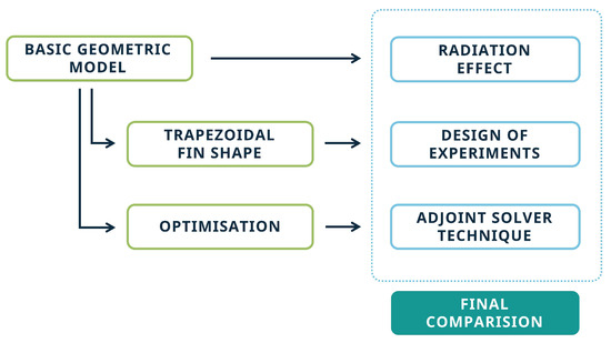
Figure 1.
The flowchart of the conducted research.
2. Research Object
The simulation of the cooling system of an electronic component is performed by the use of the simplified geometric model. The heat sink and the heat source is placed in the housing. The influence of other electronic components was neglected in the study. The geometric model of the cooling system is shown in Figure 2.
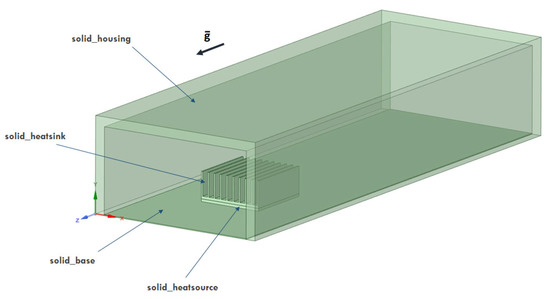
Figure 2.
Geometric model of the cooling system with names of individual parts.
The dimensions of the system are shown in projections perpendicular (Figure 3) as well as parallel (Figure 4) to the flow direction.
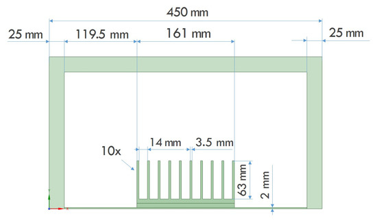
Figure 3.
Domain dimensions in front view.
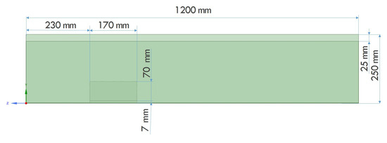
Figure 4.
Domain dimensions in side view.
It was decided to investigate the effect of modifications in the geometric model of the fins on the temperature distribution behind the heat sink and the heat source temperature. The study was performed using the DOE technique. The heat sink shape modification was determined by two parameters shown schematically in Figure 5. These are the distance of the top surface of the heat sink from the lowest point of intersection of the cutting plane with the fin (w) and the angle of inclination of the cutting plane with respect to the XY plane (). The values of the geometric parameters adopted in the simulation are shown in Table 1.
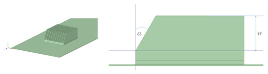
Figure 5.
Example geometric model of a trapezoidal heat sink.

Table 1.
Cutting plane parameters by which modified geometric models of the heat sink were obtained.
3. Computational Model
3.1. Mathematical Model
Heat transport in the developed cooling system is an issue described as a function of spatial coordinates. This is also a problem coupled with fluid flow. Coupling involves the conduction heat transfer from the heat source to the heat sink and to a lesser extent to the base. The heat is then transferred to the outside through natural convection and radiation.
An additional assumption can be made to simplify the mathematical model. The fluid should be considered Newtonian—its thermophysical properties in the form of conductivity, specific heat, viscosity are constant, and there are no chemical reactions or heat generation. Furthermore, the flow is assumed to be a steady-state. The following partial differential equations are solved for the problem formulated in this way:
The continuity equation can be written for the fluid:
The momentum equations are as follows:
There is heat transfer in the flow, hence energy equation to be considered is:
The calculated Rayleigh number value Ra = 2.85 for the characteristic dimension L = where S is the contact area of the heat sink and the fluid. The determined value of the Ra number does not indicate the existence of a fully turbulent flow. Many sources [42,43] give a critical Ra number of 10. However, in his work, Dixit [44] further distinguished transient flow in the Ra number range from 10 to 10. Any 2-equation turbulence model is a strong simplification of the real phenomenon of chaotic turbulence. However, failure to use an appropriate turbulence model, in this case, could lead to an incorrect description of the phenomenon under study. Turbulence model based on k (turbulent kinetic energy) and (rate of dissipation of turbulent kinetic energy) was adopted in works [45,46]. This model allows to correctly solved a cooling system using natural convection due to the lack of stability of the solution of the governing equations. Thus, in this study, the RANS turbulence modelling technique was used and—to close the Reynolds-averaged Navier–Stokes equations—the realizable model k- was assumed.
The system is also affected by radiation, which results in the use of the Surface to Surface model [47]. It is suitable for modelling the radiation in an enclosure without the participating media. Despite its limitations, this model is widely used for simple circuits.
In this study, optimization of the base shape of heat sink fins using the Adjoint Solver module is undertaken. This is a module of the Ansys Fluent package for nonparametric freeform shape optimization. Its principle of operation is based on the search for a geometric model satisfying the assumed optimization requirements.
In the initial stage of optimisation, the shape and dimensions of the geometric model are adopted by the designer. The first calculations for solving the continuity, momentum and energy equations are carried out traditionally. After determining the velocity fields and the pressure distribution, the objective function J is defined to be optimised with respect to the design parameters c [48]. Theoretically, the value of c represents the vector of all parameters that define the problem, including the locations of the grid nodes [49]. Thus, the objective function depends not only on the design parameters but also on the flow condition q(c):
The equations describing heat and mass transfer can be written in a simplified form [50]:
As the state of the flow q(c) and the control variables c change, a change in the selected optimisation objective is also observed [51]:
The first term of the above equation relates to the change in a flow state, controlled by the steady-state RANS equations, in response to a change in geometry or other boundary conditions. The Adjoint technique provides a mechanism for replacing this term with an expression that depends only on c. This replacement is achieved by exploiting the linearization of the equations describing heat and mass transfer. The optimisation should operate between defined flow field limitations: flow and design variables. Consequently, when the flow field changes, the residual variable () should remain zero [52].
In the next step, we need to obtain The Lagrange Multipliers for transforming the constrained optimization problem into an unconstrained optimization problem [53]:
Combining Equations (9) and (11) together, we get:
The value of is taken in such a way as to eliminate the influence of flow variables. This provides the adjoint equation to be solved [54]:
It is possible to obtain the dependence between cost function and design variables by inserting Equation (14) into Equation (13):
In the next step, the new shape of the geometric model is obtained by shifting the cell nodes using control nodes [55]. Subsequently, the flow analysis is repeated. Achieving the assumed value of a given objective function enables the optimisation to be successfully completed.
This optimization method has been successfully applied, for example, in the field of aerodynamics [56,57] and in solving problems coupled with heat transfer [58]. Hence, it seems fully reasonable to use this tool to optimize the shape of the heat sink.
3.2. Validation of the Adopted Model
To check the validity of the adopted mathematical model, the results of the numerical simulation were compared with the results of the experiment performed by Ruhul [59]. The exact boundary conditions, thermophysical properties of solid materials and air were assumed during validation. Furthermore, the same simulation domain, operating conditions and heat generation from the semiconductor element equal to = 2,970,000 W/m were also assumed. The role of mass forces, in this case, is played by a gravitational force in line with the direction of the z-axis, with opposite direction and a value of g = −9.81 m/s. The factor to verify both methods was the average temperature of the individual channels, i.e., the space between the ribs. The resulting temperature distribution is shown in Figure 6.
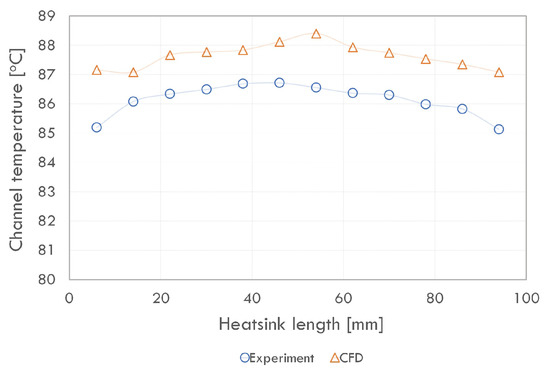
Figure 6.
Dependence of average temperature of channels on their location [59].
After analyzing the obtained distribution, it was found that the absolute error of the temperature does not exceed 2 C. Therefore, with a relative percentage error of less than 3% obtained, the model is used in subsequent calculation steps.
3.3. Computational Conditions
Appropriate boundary conditions are required to solve the governing equations. Also, computational conditions must be adopted, and a grid developed.
The airflow takes place by natural convection, so the presence of positive gauge pressure at the inlet and negative pressure at the outlet, which could force the air to move, has been neglected.
The location where the boundary conditions are adopted is shown in Figure 7. The air inlet and outlet surfaces (A and C) are characterized only by the atmospheric pressure value, with no set velocity value. This makes it possible to reproduce the natural convection. The remaining surfaces were characterized as walls with air movement between them. It was also assumed that the system was tested at an ambient temperature of 40 C; hence both at the inlet and outlet domain surface, the temperature was equal to 40 C. To represent the radiation, they were assigned emissivity values. The boundary conditions can be described as follows:
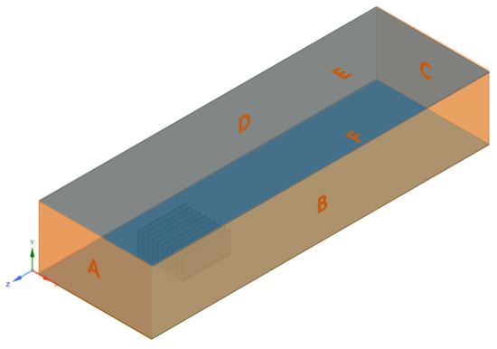
Figure 7.
Nomenclature of external planes of the domain.
- a pressure inlet type boundary condition was assumed on surface A; relative pressure value 0 Pa, surface temperature 40 C, flow direction normal to the surface;
- a pressure outlet type boundary condition was assumed on surface C; relative pressure value 0 Pa, surface temperature 40 C, flow direction normal to the surface;
- a wall type boundary condition was assumed on surfaces B, D, E, F; stationary wall, no slip (v = 0);
- the emissivity value of the outer surface of the heat sink is equal to 0.9;
- the emissivity value of the outer surface of the heat source is equal to 0.3;
- the emissivity value of the upper base surface is equal to 0.9;
- the emissivity value of the surfaces B, D, E is equal to 0.9.
The design assumption is to receive a heat flux whose value is P = 80 W. Hence, we proceeded to determine the solid_heatsource V element volume and calculated the heat generation value (Equation (16)).
Material Properties and Solver Settings
The table (Table 2) gives the assumed properties of copper, glass fibre epoxy laminate (fr-4) and heat source material. The values of specific heat, density and thermal conductivity were determined [37].
Table 2.
Determination of material properties of individual system components.
The properties of the air, which is the working medium of the cooling system, were also assumed, i.e., the specific heat c = 1006.43 J/(kgK), thermal conductivity = 0.0242 W/(mK) and dynamic viscosity = 1.7894 × 10. Given the fact of negligible pressure changes, the density of air is described by the incompressible-ideal-gas model and depends only on temperature according to the Ideal Gas Equation. Thus, the existence of a fully compressible flow can be neglected.
In a further step, the operating conditions in the domain were determined. They are characterized by a reference pressure p = 101,325 Pa, an average temperature T = 313.15 K in the domain defined by inlet and outlet conditions, and an operating density = 1.126 kg/m.
The Pseudo Transient option [37] was used in the calculations. Thus, the pseudo time step for air t = 0.37 s and copper t = 255 s was adopted in the developed cooling system model—as they have the lowest value among the time step values calculated for the other materials. Calculations were performed using a coupled pressure-based solver. A Warped-Face Gradient Correction function was used to assist in solving the equations for polyhedral grids. The interpolation scheme for pressure was adopted as Body Force Weighted, while First Order Upwind was adopted for momentum equation, turbulence kinetic energy equation, turbulence kinetic energy dissipation equation. In contrast, the Second Order Upwind scheme was chosen for the energy equation. The values of the under-relaxation parameters for pressure and momentum are 0.4; for density, mass forces, and turbulent viscosity are 1; for energy, turbulence kinetic energy and turbulence kinetic energy dissipation is 0.75. The maximum number of iterations equal to 800 or RMS (root mean square) of the residues equal to RMS = 10 were used as convergence criteria for the iterative solution scheme. Calculations were performed in ANSYS FLUENT software.
Further, numerical parameters were adopted to control the solution of the equations of the optimization algorithm. An important parameter is the Courant number. As it increases, it is possible to obtain faster convergence of the solution; however, this may mean getting an unstable solution. Obtaining a convergent solution was possible for a Courant number value of 10. Residual Minimization was used to achieve faster convergence of the solution. A convergence criterion value of 10 was set for each equation, and then the calculations were initialized. The number of iteration steps was set to 150. After 23 iteration steps, convergence was obtained for all equations (Figure 8).
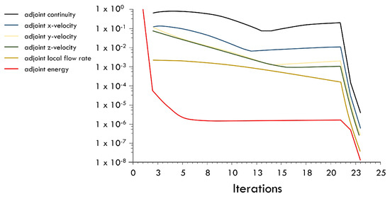
Figure 8.
Residual graphs for optimization equations.
3.4. Adopted Numerical Grid
Five poly-hexcore grids were created for the geometric model (Figure 2) differing in settings such as element size on the heat sink surface and heat source element (local_1), maximum mesh size on the surface (maximum size), and minimum mesh size (minimum size). The characteristics of all grids were collected and presented in Table 3.
Table 3.
Characteristics of numerical grids subjected to CFD analysis.
The grid independence study was examined based on parameters such as the temperature behind the heat sink (point-temperature) and the average temperature of the heat source (heatsource-temperature). The results are shown in Figure 9.
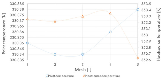
Figure 9.
Effect of the grid on the temperature value.
Figure 9 shows that the highest point temperature from all meshes was achieved for mesh no. 5. However, the temperature differences between meshes at a specific point does not exceed 0.1 K, while for the temperature of the heat source, 0.8 K. Therefore, it was decided to investigate the mass flow rate between the inlet and outlet and the total heat transfer rate between the surfaces. The results are shown in Figure 10.
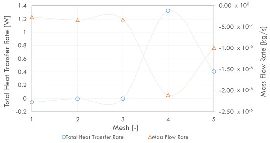
Figure 10.
Effect of the grid on the balance of streams.
Determination of the balance of individual rates for each grid allows, as it were, to confirm the fact that for grids 4 and 5, the greatest loss in mass and heat flow is observed. Hence, to obtain a correct numerical solution, it was decided to choose grid 3 (Figure 11). It is also a trade-off between the number of mesh elements and the accuracy of the solution.
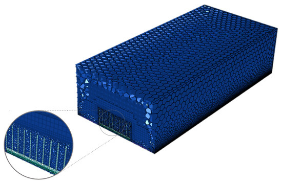
Figure 11.
Polyhexcore grid.
To select an appropriate turbulence model, the value of the y+ parameter had to be determined. A preliminary numerical simulation resulted in the dependence of the y+ parameter on the heat sink length (Figure 12). Its value is in the range of 20 to 130. Hence it is possible to apply a turbulence model that uses the wall functions—k- Realizable.
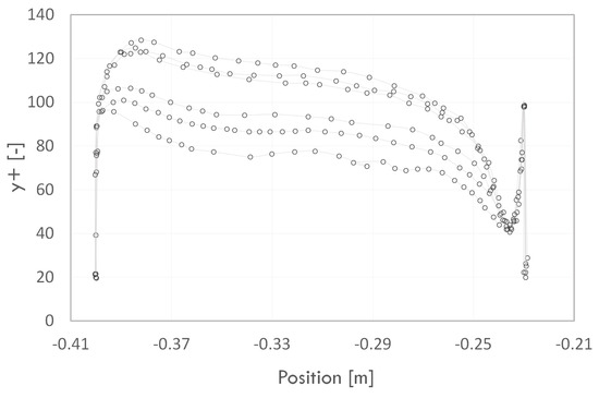
Figure 12.
Value of the y+ parameter along the length of the heat sink.
4. Results and Discussion of the Numerical Calculations
4.1. Effect of Radiation on the Solution
To develop the analysis of the results, the coordinates of the measurement point behind the heat sink need to be defined (x = 0.2125 m, y = 0.03 m, z = −0.5 m). The results of the analysis are presented as a velocity vector field in the planes parallel to the direction of motion and as a temperature field (Figure 13). The temperature scale applies to the solid domain, and the velocity scale applies to the air domain. The highest temperature value in the system of about 353 K is noted near the heat source. Slightly lower values (around 350 K) are observed on the walls of the heat sink. The base of the system—near the inlet, outlet and on the sides—is much cooler, and its temperature reaches values close to the ambient temperature. However, it can be noticed that just behind the heat sink, the area gets much hotter. This is a negative phenomenon, especially in the case when it would be decided to place another electronic component behind the heat sink. The temperature difference in the system causes natural convection. The air, starting from the inlet, flows past the heat sink, where its temperature increases. This effect reduces the air density and causes it to move towards the outlet in the direction of the z-axis. The described phenomenon can be seen in the velocity vector field. There is an increase in air velocity near the heat sink compared to its velocity at the inlet. However, it is also a fact that the velocity also increases at the outlet from the domain. Thus, the air heats up from the base wall of the system behind the heat sink. Furthermore, air streams further away from the heat sink get hotter, mainly due to the existence of the radiation phenomenon.
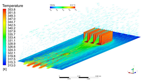
Figure 13.
Vector velocity field around the heat sink and temperature distribution of the solid type domain.
One of the convergence criteria besides the adopted residuum values was the temperature behind the heat sink and the average temperature of the heat source (Figure 14). It can be concluded that the calculation resulted in a stable value of both temperatures after 600 iterations.
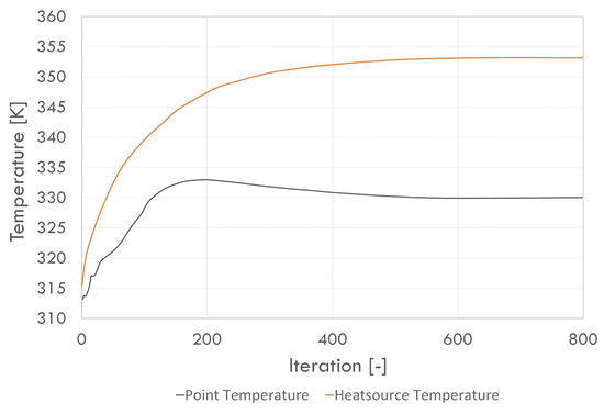
Figure 14.
Dependence of the temperature behind the heat sink (point temperature) and the average temperature of the heat source during the calculation.
The CFD analysis was also performed for the case without radiation in the system under study, and the results obtained from both analyses were compared in the form of differential temperature field (Figure 15).
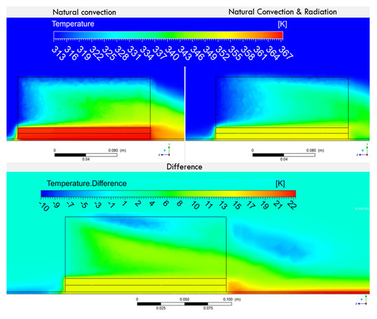
Figure 15.
Temperature distribution and the difference between simulation assuming convection and both convection and radiation.
The temperature range varied from 313 K to 367 K for the calculation assuming only natural convection. In contrast, the temperature range varied from 313 K to 355 K for the calculation assuming natural convection and radiation. The most significant differences in the temperature field are most noticeable behind the heat sink and on its surface. It can be seen (Figure 15) that the temperature difference equal 14 K and 22 K for the heat source and air behind the heat sink, respectively. Failure to account for the radiation phenomenon in the system under study leads to an overestimation of the temperature value due to the numerical model simplification.
4.2. Effect of Fin Shape on the Maximum Temperature in the Cooling System
The dependence of temperature versus section plane angle () and parameter (w) is shown in Figure 16 and Figure 17. The functions were determined by performing an approximation with second-order polynomials. The temperature behind the heat sink and the heat source temperature for the simulation before modifying the geometric model was 330.35 K and 353.15 K, respectively.
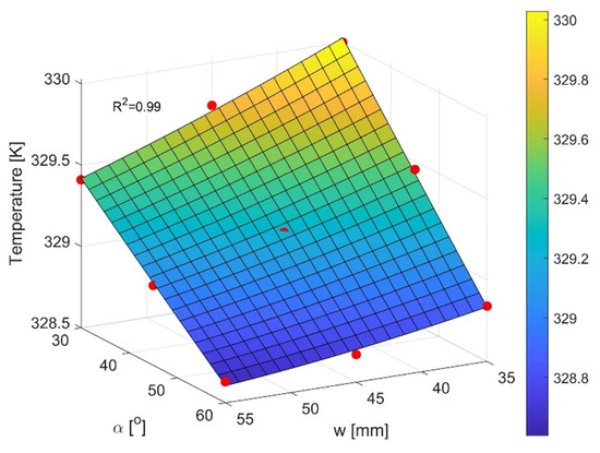
Figure 16.
Temperature dependence behind the heat sink depending on fin shape.
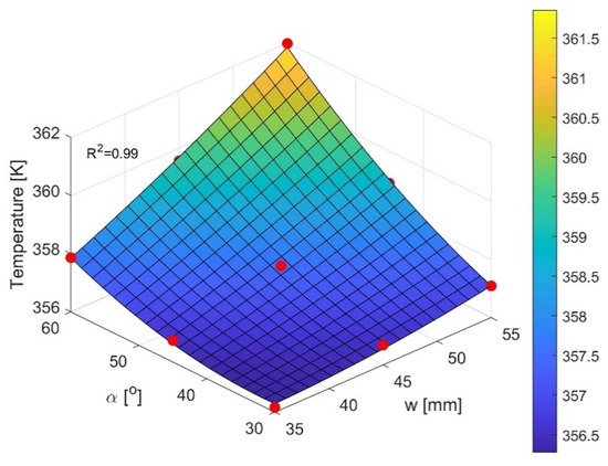
Figure 17.
Temperature dependence of the heat source depending on the case under study.
A trapezoidal fin shape reduced the temperature value behind the heat sink for each of the cases studied. It decreases with increasing angle of the section plane () and increasing (w) parameter. The maximum values of parameters () and (w) allow to decrease the value of the temperature behind the heat sink compared to the initial design by 1.5 K; however, they cause the heat source temperature to increase by 6 K. Thus, the excessive inclination of the fins negatively affects the heat source temperature value, which is related to the decrease of the heat transfer surface between the air and the heat sink. The best design in the context of minimal temperature value behind the heat sink is obtained for w = 55 mm and angle . The best design in the context of minimal heat source temperature is obtained for w = 35 mm and angle . However, finding the single best design solution requires optimization with two objective functions and is a trade-off between the temperature behind the heat sink and the heat source, and such studies have not been conducted in this research.
4.3. Use of Adjoint Solver Technique for Heat Sink Shape Optimization
The average temperature in the volume defined by the coordinates of the Box Region was assumed to be minimized. This is important because of the need to keep the temperature of the air flowing to other electronic components behind the heat sink as low as possible. A volume 0.09 m long, 0.02 m wide, and 0.02 m high are consistent with the location of the control point used to monitor the temperature behind the heat sink T (Figure 18). The initial value of the average temperature in the given volume is equal to 338.7 K.
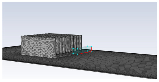
Figure 18.
Volume behind the heat sink whose average temperature is minimized.
In the next step, we evaluated the influence of the geometric model of the heat sink on the value of the adopted optimization criterion. To this end, log10 (Shape Sensitivity Magnitude) field was prepared on the surfaces of the heat sink, the electronic component and the base. Based on this, it was found that changing the shape of the back of the fins at the bottom base would have the greatest effect on reducing the temperature values behind the heat sink (Figure 19). The sensitivity of a variable to the value of mass forces exerted on a numerical grid cell can be similarly represented (Figure 20). The shape change area in the optimization process was assumed to be a cuboid encompassing the boundaries of the entire heat sink, taking into account the possibility of changing the shape of the geometric model near the edges of the fins as shown on the log10 field (Figure 19).
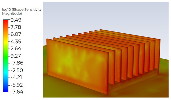
Figure 19.
Sensitivity of heat sink shape expressed by the log10 function.
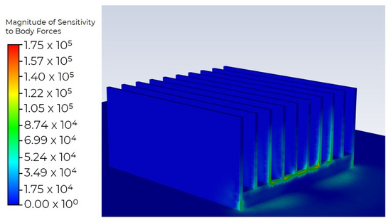
Figure 20.
Sensitivity of the optimization criterion to mass forces.
For the current calculations, the number of control nodes was increased to perform more accurate changes to the geometric model. For the x-direction, 40 points were determined; for the y-direction and z-direction, 30 points were determined. A Freeform Scale Factor, which allows the magnitude of the attempted design change to be adjusted, equal to 2, was also assumed. After the initial calculation, the percentage value of the expected improvement of the optimization criterion was determined. The numerical grid transformed in the given iterative step was then modified. In the next step, calculations were carried out in ANSYS Fluent (taking into account the radiation phenomenon), and the optimization was performed again. In this way, 21 iterations were implemented, during which the geometric model of the heat sink was optimized to reduce the temperature behind the heat sink.
Figure 21 shows the temperature trend behind the heat sink, both the approximate temperature determined in the optimization process (orange) and the actual temperature verified in ANSYS Fluent (blue). The change in the optimization criterion under study is presented over successive iterations.
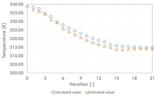
Figure 21.
Temperature change behind the heat sink for 21 iterations.
From Figure 21, the positive effect of performing the optimization can be observed. The set temperature value has decreased from about 340 K to 315 K. Thus, it can be concluded that it corresponds to the inlet and outlet conditions. Hence further improvement is practically impossible. With each iteration, a decrease in the minimum orthogonal quality of the generated division grid is observed, which negatively affects the calculations and limits the number of possible iterations in the optimization process (Figure 22).
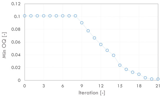
Figure 22.
Change in minimum orthogonal quality over successive iterations.
The trend of the maximum temperature of the heat source was also investigated (Figure 23). Its value also decreased, however, not as much as the air temperature behind the heat sink. Over the iterations, the value of the studied temperature changed by a maximum of about 0.3 K. Hence, modifying the geometric model to lower the temperature behind the heat sink does not adversely affect the thermal performance of the heat source. An inverse relationship between both temperatures was observed during the numerical simulation of heat sinks with trapezoidal fins.
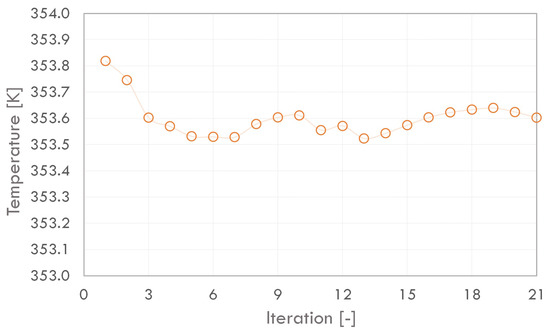
Figure 23.
Change in maximum temperature of electronic component.
Figure 24 shows the change in the shape of the geometric model in selected optimisation steps and the temperature distribution on the heat sink surface and on the system base plane. The observed differences correspond to the projections included in the sensitivity fields (Figure 19 and Figure 20). In the initial iterations, the geometric model of the heat sink does not change significantly. In the 8th iteration, a bending of the back part of the fins can be observed. In the 16th iteration, this change deepens and additionally begins to include also the fins located on the outer side. The modification of the geometrical model also decreases the temperature of the base behind the heat sink. Although up to the 8th iteration, the value of this temperature practically does not change, in subsequent iterations, it is already below 320 K. Additionally, a differential temperature distribution was developed between the 1st and 21st iteration steps (Figure 25). The results are presented on a plane parallel to the base plane, offset by 0.03 m according to the OY-axis direction. From this, it can be concluded that the optimisation performed not only contributed to lowering the temperature just behind the heat sink (by about 25 K) but also made it possible to reduce it in a much larger area behind the heat source. In these areas, the temperature difference is as much as 10 K. This makes it possible, in practice, to place another component that would require appropriate temperature conditions during its operation. Furthermore, a reduction in temperature values in any volume (not only in the immediate vicinity of the heat sink) can be given as an objective in this type of optimisation, depending on the design assumptions.
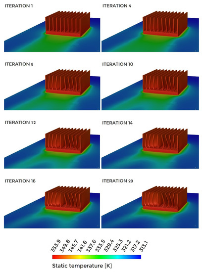
Figure 24.
Change in heat sink shape and temperature distribution.
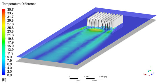
Figure 25.
Differential temperature distribution between the first and last iteration.
4.4. Effect of Power Dissipated by an Element on the Temperature in the Cooling System
In this study, the temperature dependence of the heat source and the temperature behind the heat sink versus the power generated by the electronic component was determined. The characteristics were plotted for three geometric models: the base model (Figure 2), the trapezoidal heat sink for parameter w = 55 mm and = 60, and the optimal shape (solution for 16 iterations). The assumed value of the heat generation in the electronic component is shown in Table 4.
Table 4.
Assumed value of the heat generation in the electronic component.
Summary results for all heat sink shape cases in terms of the temperature dependence behind the heat sink versus heat flux are shown in Figure 26. A similar relationship, however, in this case for the heat source temperature, is presented in Figure 27.
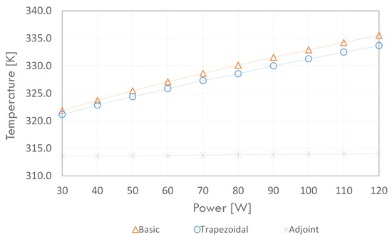
Figure 26.
Temperature dependence behind the heat source versus heat flux.
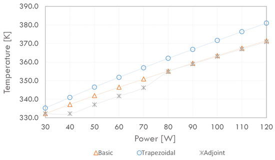
Figure 27.
Temperature dependence of the heat source versus heat flux.
By analyzing Figure 26 and Figure 27 it can be observed that the temperature value increases with the increase of generated power. The temperature value behind the heat sink is highest for the basic heat sink, while the cooling system using the trapezoidal fins has lower temperature values for the entire power range. Notably, the temperature behind the heat sink decreases significantly for the geometric model of the heat sink optimized in Adjoint Solver. For the entire power range, a nearly constant value of this temperature is observed equally to the inlet and outlet conditions. The temperature dependence of the heat source follows a similar pattern; however, higher values are recorded for trapezoidal fin shapes. For powers lower than 80 W, significant reductions in source temperature were achieved.
We decided to compare three geometric models: a basic heat sink, a heat sink with trapezoidal fins (w = 55 mm, = 60) and a heat sink optimised using the Adjoint Solver technique for a heat source power of 70 W. The results were presented in a plane parallel to the XZ plane for y = 0.03 m. A velocity vector field was used for comparison, and the temperature values were plotted on it (Figure 28).
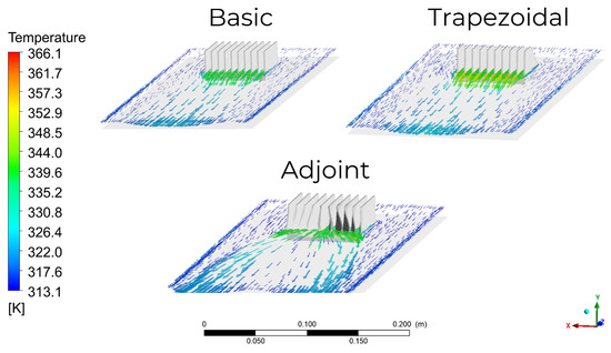
Figure 28.
Comparison of flow direction and temperature field for three geometric models of a heat sink.
From Figure 28 we conclude that the direction of the velocity vectors behind the basic heat sink and the heat sink with trapezoidal fins is similar. In the case of the heat sink optimised with the Adjoint Solver technique, the airflow is divided into two parts at the back of the domain. This results in a lower temperature of the airflow in the central part of the system behind the heat sink, compared to the other cases. It can also be noted that the temperature values for the systems with the basic heat sink and the heat sink with trapezoidal fins have a similar distribution. Hence, we decided to compare the temperature change behind the heat sink for the three geometric models. Consequently, a chart (Figure 29) was made basic on a centre line of the velocity field plane (for constant values of x = 0.2125 m, y = 0.03 m and a change in value of z value from −0.4 m to −1.2 m).
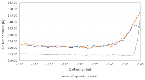
Figure 29.
Comparison of the temperature dependence behind the heat sink.
In comparing the basic and the trapezoidal fins heat sinks, it is found that the temperature change in the backside is similar. Lower temperature values are observed behind the basic heat sink, but in the latter part, its average value is already higher. At the outlet of the system, a temperature drop behind the basic heat sink is visible compared to the temperature behind the trapezoidal heat sink. The use of a heat sink with an optimised shape by using the Adjoint Solver technique allows a significant reduction in temperature in the rear part of the system—on average by 5 K. The best design in the context of minimal temperature value behind the heat sink from all analysed cases is obtained for heat sink with deformed fins according to iteration 14 (Figure 24). The further modifications do not improve the solution.
5. Summary and Conclusions
This study presents the results of numerical calculations of the problem of cooling electronic components in a confined space. Analyses were performed using the RANS technique taking into account the natural convection and radiation. The authors present the results of optimizing the shape of the geometric model using the Adjoint Solver technique and analyzing the effect of the power dissipated by the electronic component on the temperature in the cooling system. An analysis of the effect of radiation in the cooling process simulation on the solution was also performed, and the effect of the trapezoidal shape of the fins on the maximum temperature in the cooling system was investigated. The major findings of the study are presented in several sections:
- The optimisation performed using the Adjoint Solver technique allowed for a reduction of the assumed temperature by 25 K. This did lead to a decrease in the minimum value of the orthogonal grid quality. However, in this case, it is possible to re-generate the grid for the optimised geometric model.
- Neglecting the radiation phenomenon in the tested system led to overestimated heat sink temperatures (by nearly 14 K).
- Increasing the angle of the fin () and increasing the value of the parameter (w) allows a lower value of the air temperature behind the heat sink, which on the other hand, adversely affects the heating of the heat source component. The maximum values of the parameters and w cause a 1.5 K decrease in the temperature value behind the heat sink and a 6 K increase in the heat source temperature.
- The proposed optimal fin design ensures that the increase in heat source power does not significantly affect the temperature in the area behind the heat sink.
- The heat source temperature for optimal fin design and heat flux up to 80 W is lower than the basic design and trapezoidal fins.
Despite its ability to investigate heat transport problems, the Adjoint Solver technique combined with Ansys Fluent has some limitations: sensitivity to mesh element size and inability to perform transient calculations, not considering the phase change model or the radiation phenomenon. As a further direction of this research, the authors propose to perform a similar optimisation for a different type of heat sink (for example, with pin fins) and consider the influence of other boundary conditions on the model’s shape optimised using the Adjoint Solver technique.
Author Contributions
Conceptualization, G.C.; Investigation, G.C.; Methodology, G.C. and J.W.; Supervision, J.W.; Validation, G.C.; Writing—original draft, G.C. and J.W. Both authors have read and agreed to the published version of the manuscript.
Funding
This research received no external funding.
Institutional Review Board Statement
Not applicable.
Informed Consent Statement
Not applicable.
Data Availability Statement
Data sharing not applicable.
Acknowledgments
This research was supported by national subvention no. 16.16.130.942.
Conflicts of Interest
The authors declare no conflict of interest.
Abbreviations
The following abbreviations are used in this manuscript:
| c | specific heat of fluid [J/(kg·K)], design parameters, |
| gravitational acceleration in a given direction [m/s], | |
| J | objective function, |
| k | turbulent kinetic energy [m/s], |
| L | Lagrangian function, |
| p | pressure [Pa], |
| q | heat generation [W/m], flow condition function, |
| R | residual variable, |
| T | temperature [K], |
| t | time [s], |
| t | pseudo time step [s], |
| ,, | Cartesian velocity coordinates [m/s], |
| w | fins height [mm], |
| x, y, z | Cartesian coordinates [m], |
| angle of inclination [], | |
| rate of dissipation of turbulent kinetic energy [m/s], | |
| fluid thermal conductivity [W/(m·K)], vector of adjoint variables, | |
| fluid dynamic viscosity [Pa·s], | |
| fluid density [kg/m] |
References
- Sui, Y.; Teo, C.J.; Lee, P.S.; Chew, Y.T.; Shu, C. Fluid flow and heat transfer in wavy microchannels. Int. J. Heat Mass Trans. 2010, 53, 2760–2772. [Google Scholar] [CrossRef]
- Sivasamy, A.; Selladurai, V.; Kanna, P.R. Mixed convection on jet impingement cooling of a constant heat flux horizontal porous layer. Int. J. Therm. Sci. 2010, 49, 1238–1246. [Google Scholar] [CrossRef]
- Starner, K.E.; McManus, H.N., Jr. An Experimental Investigation of Free-Convection Heat Transfer From Rectangular-Fin Arrays. J. Heat Transf. 1963, 85, 273–277. [Google Scholar] [CrossRef]
- Chaddock, J.B. Free convection heat transfer from vertical rectangular fin arrays. ASHRAE J. 1970, 12, 53–60. [Google Scholar]
- Leung, C.W.; Probert, S.D.; Shilston, M.J. Heat exchanger: Optimal separation for vertical rectangular fins protruding from a vertical rectangular base. Appl. Energy 1985, 19, 77–85. [Google Scholar] [CrossRef]
- Leung, C.W.; Probert, S.D.; Shilston, M.J. Heat exchanger design: Optimal uniform separation between rectangular fins protruding from a vertical rectangular base. Appl. Energy 1985, 19, 287–299. [Google Scholar] [CrossRef]
- Leung, C.W.; Probert, S.D.; Shilston, M.J. Heat transfer performances of vertical rectangular fins protruding from rectangular bases: Effect of fin length. Appl. Energy 1986, 22, 313–318. [Google Scholar] [CrossRef]
- Leung, C.W.; Probert, S.D. Heat-exchanger performance: Effect of orientation. Appl. Energy 1989, 33, 235–252. [Google Scholar] [CrossRef]
- Leung, C.W.; Probert, S.D. Thermal effectiveness of short-protrusion rectangular, heat-exchanger fins. Appl. Energy 1989, 34, 1–8. [Google Scholar] [CrossRef]
- de Lieto Vollaro, A.; Grignaffi, S.; Gugliermetti, F. Optimum design of vertical rectangular fin arrays. Int. J. Therm. Sci. 1999, 38, 525–529. [Google Scholar] [CrossRef]
- Baskaya, S.; Sivrioglu, M.; Ozek, M. Parametric study of natural convection heat transfer from horizontal rectangular fin arrays. Int. J. Therm. Sci. 2000, 39, 797–805. [Google Scholar] [CrossRef]
- Harahap, F.; Setio, D. Correlations for heat dissipation and natural convection heat-transfer from horizontally-based, vertically-finned arrays. Appl. Energy 2001, 69, 29–38. [Google Scholar] [CrossRef]
- Edwards, J.A.; Chaddock, J.B. An experimental investigation of the radiation and free convection heat transfer from a cylindrical disk extended surface. ASHRAE Trans. 1963, 69, 313–322. [Google Scholar]
- Azarkish, H.; Sarvari, S.M.H.; Behzadmehr, A. Optimum geometry design of a longitudinal fin with volumetric heat generation under the influences of natural convection and radiation. Energy Convers. Manag. 2010, 51, 1938–1946. [Google Scholar] [CrossRef]
- Rao, V.D.; Naidu, S.V.; Rao, B.G.; Sharma, K.V. Heat transfer from a horizontal fin array by natural convection and radiation—A conjugate analysis. Int. J. Heat Mass Transf. 2006, 49, 3379–3391. [Google Scholar] [CrossRef]
- Wu, Y.; Gao, N.; Niu, J.; Zang, J.; Caoa, Q. Numerical study on natural ventilation of the wind tower: Effects of combining with different window configurations in a low-rise house. Build. Environ. 2021, 188, 107450. [Google Scholar] [CrossRef]
- Soltani, M.; Dehghani-Sanij, A.; Sayadnia, A.; Kashkooli, F.M.; Gharali, K.; Mahbaz, S.; Dusseault, M.B. Investigation of Airflow Patterns in a New Design of Wind Tower with a Wetted Surface. Energies 2018, 11, 1100. [Google Scholar] [CrossRef] [Green Version]
- Mehryan, S.A.M.; Kashkooli, F.M.; Soltani, M. Comprehensive study of the impacts of surrounding structures on the aero-dynamic performance and flow characteristics of an outdoor unit of split-type air conditioner. Build. Simul. 2018, 11, 325–337. [Google Scholar] [CrossRef]
- Kashkooli, F.M.; Soltani, M.; Zargar, B.; Ijaz, M.K.; Taatizadeh, E.; Sattar, S.A. Analysis of an indoor air decontamination device inside an aerobiology chamber: A numerical-experimental study. Air Qual. Atmos. Health 2020, 13, 281–288. [Google Scholar] [CrossRef]
- Kashkooli, F.M.; Sefidgar, M.; Soltani, M.; Anbari, S.; Shahandashti, S.-A.; Zargar, B. Numerical Assessment of an Air Cleaner Device under Different Working Conditions in an Indoor Environment. Sustainability 2021, 13, 369. [Google Scholar] [CrossRef]
- Xie, Z.; Xiao, Y.; Jiang, C.; Ren, Z.; Li, X.; Yu, K. Numerical research on airflow-dust migration behavior and optimal forced air duct installation position in a subway tunnel during drilling operation. Powder Technol. 2021, 388, 176–191. [Google Scholar] [CrossRef]
- Tari, I.; Mehrtash, M. Natural convection heat transfer from inclined plate-fin heat sinks. Int. J. Heat Mass Transf. 2013, 56, 574–593. [Google Scholar] [CrossRef]
- Kim, T.H.; Kim, D.-K.; Do, K.-H. Correlation for the fin Nusselt number of natural convective heat sinks with vertically oriented plate-fins. Heat Mass Transf. 2013, 49, 413–425. [Google Scholar] [CrossRef]
- Kulkarni, V.M.; Dotihal, B. CFD and conjugate heat transfer analysis of heat sinks with different fin geometries subjected to forced convection used in electronics cooling. Int. J. Res. Eng. Technol. 2013, 4, 158–163. [Google Scholar]
- Maji, A.; Bhanja, D.; Patowari, P.K. Numerical investigation on heat transfer enhancement of heat sink using perforated pin fins with inline and staggered arrangement. Appl. Therm. Eng. 2017, 125, 596–616. [Google Scholar] [CrossRef]
- Shadlaghani, A.; Tavakoli, M.R.; Farzaneh, M.; Salimpour, M.R. Optimization of triangular fins with/without longitudinal perforate for thermal performance enhancement. J. Mech. Sci. Technol. 2016, 30, 1903–1910. [Google Scholar] [CrossRef]
- Al-Sallami, W.; Al-Damook, A.; Thompson, H.M. A numerical investigation of the thermal-hydraulic characteristics of perforated plate fin heat sinks. Int. J. Therm. Sci. 2017, 121, 266–277. [Google Scholar] [CrossRef] [Green Version]
- Saraiya, A.; Chandramohan, V.P.; Balasubramanian, K. Optimization of Horizontal Rectangular Fin Heat Sink: A CFD with Response Surface Analysis and Parametric Study. J. Inst. Eng. India 2020, 101, 149–158. [Google Scholar] [CrossRef]
- Patel, H.; Matawala, V.K. Performance Evaluation and parametric optimization of a Heat Sink for Cooling of Electronic Devices with Entropy Generation Minimization. Eur. J. Sustain. Dev. Res. 2019, 3, em0100. [Google Scholar] [CrossRef]
- Iradukunda, A.-C.; Vargas, A.; Huitink, D.; Lohan, D. Transient thermal performance using phase change material integrated topology optimized heat sinks. Appl. Therm. Eng. 2020, 179, 115723. [Google Scholar] [CrossRef]
- Feppon, F.; Allaire, G.; Dapogny, C.; Jolivet, P. Body-fitted topology optimization of 2D and 3D fluid-to-fluid heat exchangers. Comput. Methods Appl. Mech. Eng. 2021, 376, 113638. [Google Scholar] [CrossRef]
- Sun, S.; Liebersbach, P.; Qian, X. 3D topology optimization of heat sinks for liquid cooling. Appl. Therm. Eng. 2020, 178, 115540. [Google Scholar] [CrossRef]
- Nemati, H.; Moghimi, M.A.; Sapin, P.; Markides, C.N. Shape optimisation of air-cooled finned-tube heat exchangers. Int. J. Therm. Sci. 2020, 150, 106233. [Google Scholar] [CrossRef]
- Menrath, T.; Rosskopf, A.; Simon, F.B.; Groccia, M.; Schuster, S. Shape Optimization of a Pin Fin Heat Sink. In Proceedings of the 36th Semiconductor Thermal Measurement, Modeling & Management Symposium, San Jose, CA, USA, 16–20 March 2020. [Google Scholar]
- Ghosh, S.; Mondal, S.; Fernandez, E.; Kapat, J.S.; Roy, A. Parametric Shape Optimization of Pin-Fin Arrays Using a Surrogate Model-Based Bayesian Method. In Proceedings of the American Institute of Aeronautics and Astronautics AIAA Propulsion and Energy 2019 Forum, Indianapolis, IN, USA, 19–22 August 2019. [Google Scholar]
- Das, S.; Sutradhar, A. Multi-physics topology optimization of functionally graded controllable porous structures: Application to heat dissipating problems. Mater. Des. 2020, 193, 108775. [Google Scholar] [CrossRef]
- Lee, J.S.; Ha, M.Y.; Min, J.K. A finite-volume based topology optimization procedure for an aero-thermal system with a simplified sensitivity analysis method. Int. J. Heat Mass Transf. 2020, 163, 120524. [Google Scholar] [CrossRef]
- Høghøj, L.C.; Nørhave, D.R.; Alexandersen, J.; Sigmund, O.; Andreasen, C.S. Topology optimization of two fluid heat exchangers. Int. J. Heat Mass Transf. 2020, 163, 120543. [Google Scholar] [CrossRef]
- Lee, G.; Lee, I.; Kim, S.J. Topology optimization of a heat sink with an axially uniform cross-section cooled by forced convection. Int. J. Heat Mass Transf. 2021, 168, 120732. [Google Scholar] [CrossRef]
- Zeng, T.; Wang, H.; Yang, M.; Alexandersen, J. Topology optimization of heat sinks for instantaneous chip cooling using a transient pseudo-3D thermofluid model. Int. J. Heat Mass Transf. 2020, 154, 119681. [Google Scholar] [CrossRef] [Green Version]
- Lee, J.S.; Yoon, S.Y.; Kim, B.; Lee, H.; Ha, M.Y.; Min, J.K. A topology optimization based design of a liquid-cooled heat sink with cylindrical pin fins having varying pitch. Int. J. Heat Mass Transf. 2021, 172, 121172. [Google Scholar] [CrossRef]
- Dhar, P.L. Review of Fundamentals. In Thermal System Design and Simulation; Lisa Reading; Academic Press: Cambridge, MA, USA, 2017; p. 129. [Google Scholar]
- Cengel, Y. Natural Convection. In Heat and Mass Transfer: A Practical Approach, 3rd ed.; McGraw-Hill: New York, NY, USA, 2006; p. 467. [Google Scholar]
- Dixit, H.N.; Babu, V. Simulation of high Rayleigh number natural convection in a square cavity using the lattice Boltzmann method. Int. J. Heat Mass Transf. 2006, 49, 727–739. [Google Scholar] [CrossRef]
- Lampio, K. Optimization of Fin Arrays Cooled by Forced or Natural Convection. Ph.D. Thesis, Tampere University of Technology, Tampere, Finland, 2018. [Google Scholar]
- Meng, X.; Zhu, J.; Wei, X.; Yan, Y. Natural convection heat transfer of a straight-fin heat sink. Int. J. Heat Mass Transf. 2018, 123, 561–568. [Google Scholar] [CrossRef]
- ANSYS FLUENT 12.0 User’s Guide. Available online: https://www.afs.enea.it/project/neptunius/docs/fluent/html/th/node116.htm (accessed on 20 December 2020).
- Schramm, M.; Stoevesandt, B.; Peinke, J. Optimization of Airfoils Using the Adjoint Approach and the Influence of Adjoint Turbulent Viscosity. Computation 2018, 6, 5. [Google Scholar] [CrossRef] [Green Version]
- Wang, M.; Wang, Q.; Zaki, T.A. Discrete adjoint of fractional-step incompressible Navier-Stokes solver in curvilinear coordinates and application to data assimilation. J. Comput. Phys. 2019, 369, 427–450. [Google Scholar] [CrossRef]
- Lang, M. CFD-Method for 3D Aerodynamic Adjoint Simulations. Master’s Thesis, Linkoping University, Linkoping, Sweden, 2019. [Google Scholar]
- Roth, R.; Ulbrich, S. A Discrete Adjoint Approach for the Optimization of Unsteady Turbulent Flows. Flow Turbul. Combust. 2013, 90, 763–783. [Google Scholar] [CrossRef]
- Gkaragkounis, K.T. Conjugate Heat Transfer Shape Optimization Based On The Continuous Adjoint Method. In Proceedings of the International VII International Conference on Computational Methods for Coupled Problems in Science and Engineering (COUPLED 2017), Rhodes Island, Greece, 12–14 June 2017. [Google Scholar]
- Sen, A.; Towara, M.; Naumann, U. Sensitivity computation for ducted flows using adjoint of implicit pressure-velocity coupled solver based on Foam. In Proceedings of the Eurogen, Glasgow, UK, 14–16 September 2015. [Google Scholar]
- Tzanakis, A. Duct optimization using CFD software ‘ANSYS Fluent Adjoint Solver’. Master’s Thesis, Chalmers University of Technology, Goteborg, Sweden, 2014. [Google Scholar]
- Plutecki, Z.; Sattler, P.; Ryszczyk, K. Innowacyjny proces projektowania i optymalizacji produktów z wykorzystaniem solvera Adjoint. In Proceedings of the Innowacje w Zarządzaniu i inżYnierii Produkcji, Zakopane, Poland, 1–3 March 2015; Volume 18. [Google Scholar]
- Kalinowski, M.; Szczepanik, M. Aerodynamic Shape Optimization of Racing Car Front Wing; IOP Conference Series: Materials Science and Engineering; IOP Publishing Ltd.: Bristol, UK, 2021; Volume 1037. [Google Scholar]
- Day, H.; Ingham, D.; Ma, L.; Pourkashanian, M. Adjoint based optimisation for efficient VAWT blade aerodynamics using CFD. J. Wind Eng. Ind. Aerodyn. 2021, 208, 104431. [Google Scholar] [CrossRef]
- Towara, M.; Lotz, J.; Naumann, U. Discrete adjoint approaches for CHT applications in OpenFOAM. Comput. Methods Appl. Sci. 2021, 55, 163–178. [Google Scholar]
- Rana, R.A. Numerical and Experimental Study on Orientation Dependency of Free Convection Heat Sinks. Master’s Thesis, The University of British Columbia, Okangan, BC, Canada, 2015. [Google Scholar]
Publisher’s Note: MDPI stays neutral with regard to jurisdictional claims in published maps and institutional affiliations. |
© 2021 by the authors. Licensee MDPI, Basel, Switzerland. This article is an open access article distributed under the terms and conditions of the Creative Commons Attribution (CC BY) license (https://creativecommons.org/licenses/by/4.0/).