Analysis of the Potential for Reducing Life Cycle Greenhouse Gas Emissions from Motor Fuels

Abstract

The assessment of life cycle greenhouse gas emissions of motor fuels is important due to the legal obligations and corporate social responsibility of the petroleum industry. Combining the Life-Cycle Assessment with optimization methods can provide valuable support in the decision-making process. In this paper, a mathematical model of a refinery was developed to analyze the impact of process optimization on GHG emissions at the fuel production stage. The model included ten major refinery units. Fuel production costs were minimized by taking into account the number of constraints. The analysis was performed in two steps. First, the model was run for the reference case of fuels composition. Then, more than twelve thousand model runs were performed. In each model, the fuel composition was changed. This change represented the exogenous pressures and resulted in different flows of mass, energy and GHG emission at the refinery. The most favorable results in terms of GHG emissions were then identified and analyzed. Additionally, the impact of using low-carbon fuels for process heating was evaluated. The study showed that fuel blending management could lead to the reduction of GHG emissions by 0.4 gCO₂-eq/MJ while the use of low-carbon fuel for process heating results in a reduction of GHG emissions by 2 ca. gCO₂-eq/MJ.

1. Introduction

Crude oil is the basic raw material for the production of motor fuels, as well as other products necessary to meet economic needs. After being extracted and purified crude oil is sent to refineries where it undergoes physical and physicochemical processes. Motor fuels are composed of crude oil fractions processed in refinery installations, biofuel and additives, which are added so they can meet the specific quality requirements. The directions of development of motor fuels are mainly determined by energy and climate policy, as well as by the continuous development of car engine designs [1,2]. The findings in [3] indicate that, in both China and the US, liquid fuels maintain their dominant position in transportation, while biofuels and electric vehicles support the decarbonization of that sector. Continuous improvements in energy efficiency of technological process, as well as economic considerations and increased quality requirements for petroleum products are forcing deeper processing of crude oil. Increasing crude oil processing requires more energy, which generates increased GHG emissions. On the other hand, high quality fuels can be burned in modern efficient car engines, which in turn, contributes to the reduction of GHG emission from combustion. Bearing in mind the above, the proper assessment of the GHG emission reduction, requires the methodology of the product life cycle assessment (LCA Life Cycle Assessment [4,5]). LCA allows for the comprehensive assessment of each product taking into account the emission generated both at the stage of raw material acquisition and product utilization. According to the Fuel Quality Dirctive (FQD) [6], EU Member States require suppliers to reduce life cycle greenhouse gas emissions per unit of energy derived from fuels. The life cycle of motor fuels covers processes performed by various independent economic entities, located in different parts of the world. However, the obligation to reduce GHG emission, according to the legislation [6,7,8] is imposed on fuel suppliers, i.e., refineries which are managing only one of the stages in the life cycle. Therefore, the calculations carried out within the framework of this work focus only on feasible pathways of GHG emission reduction for the refinery stage.

In order to identify the best options for GHG emission reduction, it is necessary to identify the emission sources and develop a mathematical model reflecting the flows of mass and energy streams in the refinery. The relationship between fuel composition and the determined average value of GHG emission allocated to the fuels, as well as external constraints, such as demand and quality requirements must be considered. The main source of GHG emission at the stage of crude oil processing are emissions resulting from the production and use of energy for processing purposes. Energy carriers are most often heating fuels, electricity and energy contained in technological steam. Each of these carriers is characterized by a different GHG emission factors in relation to energy content. Therefore, one of the important issues considered in this work was also the assessment of the impact of change of energy carriers to the low-emission ones at the stage of refinery. At present, the use of biofuel is a key way to reduce GHG emission in the life cycle of motor fuels. Recent advances in the sustainability analysis of biofuel, in the form of LCA, include increased incorporation of spatially explicit elements of feedstock growth, including changes in soil carbon and fertilization rates [9]. The effectiveness of this pathway was assessed within this work. It should be noted that the RED II directive [10] imposes the upper limit (up to 7% of energy share) of biofuel content obtained from agricultural raw materials. At the same time RED II puts a great emphasis on using the biofuels produced from waste materials, setting the target of minimum 3.5% of the content of such biofuels in the year 2030, and counting their energy value as double. However, double counting of the energy content of those fuels to the target determined in the RED II directive does not correlate with reliefs or incentives resulting from the use of those fuels to reach the goals of the FQD directive. For this reason, among others, it is also necessary to look for other pathways of the life cycle GHG emission reduction.

Rising environmental awareness and stricter requirements to reduce the environmental impact of modern society are prompting research that considers environmental impacts as an additional design factor in optimizing energy supply systems at different scales. For instance, in the study [11], an optimization model was built for national energy system development that considered environmental and health impact. An approach to combine multiple objectives, in order to determine the optimal configuration of the local energy system, has been explored in [12].

This paper describes the mathematical optimization model developed for managing the GHG emission over the life cycle of motor fuels. The combination of the LCA methodology with optimization techniques is the next step in the development of tools supporting decision-making processes, especially in the aspect of pro-environmental activities. Due to the inability to influence fuel suppliers and customers, the model considered the refinery—crude processing stage—and assumed constant GHG emission rates for the other stages. Typically, optimization models in the chemical industry and engineering applications focus on optimization of economic objective functions [13,14]. A study [15] presents the results of the developed computational model, which was used to assess the increase in CO₂ emissions resulting from the reduction of sulfur content in fuels. In general, the approach to the problem of incorporating LCA into optimization consists of three main steps: (i) Conducting a life cycle assessment study, (ii) formulating and solving an optimization problem, and (iii) selecting the most advantageous solution. It is important that the developed model does not solve only a specific problem of one refinery, but has a universal character and can be applied in many enterprises. For this reason, it was decided that a model would be developed using the TIMES model generator. TIMES has been developed within the ETSAP program operating within the structures of the IEA (International Energy Agency) [16]. It belongs to the group of bottom-up optimization models. TIMES has been used in several hundred projects in over 70 countries. It is one of the main tools supporting the development of energy strategies in the European Union [17,18]. Due to its broad capabilities, it has also been used for assessing the impact of indirect emissions from equipment and infrastructure in their life cycle impacts on selected GHG emission reduction pathways [19] and to assess the impact of technology diffusion on energy and CO₂ reduction to 2050 [20]. TIMES was used in the USA and China to model the transport sector decarbonisation [21]. Such a wide application of this generator, well described and verifiable methodology is undoubtedly its great advantage. It also models refineries, but in a simplified way [22]. In this study, a detailed refinery model was developed including 10 refinery installations, i.e., atmospheric distillation, vacuum distillation, hydrocracking, hydrodesulfurization of diesel and gasoline, reforming, isomerization, hydrogen production, liquid gas department, as well as fuel blending unit. The capabilities of the model were demonstrated in the case study of a real refinery. A series of refinery system simulations were conducted to obtain the solutions characterized by the lowest average value of GHG emission allocated to the fuels.

To the best of the authors’ knowledge, no study has so far attempted to create the model of a single refinery using TIMES generator with such a detailed representation of processing units and blending facilities. One of conclusions in [23] was that the entire carbon footprints of refinery products are mostly affected by approaches to refinery modelling especially regarding the methods applied to assign shares of the total burden from the refinery operation to the individual products. The use of the linear programming model for allocation of CO₂ emissions in refineries to petroleum products was demonstrated in [24]. The variations of refinery GHG emissions allocated to oil products for different allocating methods were analyzed by [25]. Although, in this paper, we use only one energy-based allocation method its novelty is that we explore how the change in refinery settings in terms of activities and commodity flows between processing units can contribute to reduction of GHG emissions assigned to motor fuels. We also contribute by providing the new set of results for refinery GHG emissions allocated to the motor fuels, which is complementary to the studies such as the ones presented in [23].

The main achievements of the research are:

-

development of a refinery model using TIMES generator with a detailed representation of processing units and blending facilities,

-

development of the modelling system that made it possible to run a series of refinery simulations with exogenously determined fuel composition to identify the solutions characterized by the lowest average value of GHG emission assigned to motor fuels,

-

demonstration of new approach to fuels production management by using a tool that incorporates refinery processing optimization into LCA of motor fuels,

-

new set of results for refinery GHG emissions allocated to the motor fuels.

2. Materials and Methods

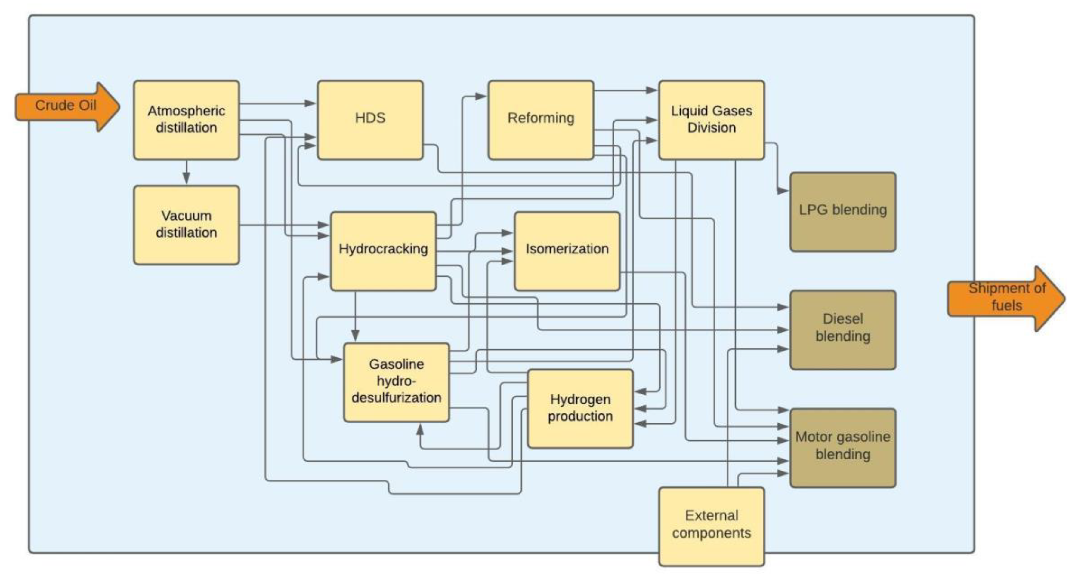
The purpose of this paper was to evaluate the improvement in the life cycle GHG emission reduction pathways for motor fuels at the refinery production stage. The work had a research and analytical character and concerned the simulation of GHG emission reduction based on a mathematical computational model, for different paths of GHG emission reduction. The object of the research was a real refinery of LOTOS Group S.A. in Gdańsk/Poland reflected in the model with a simplified scheme. However, the principles of building the model, determining allocation coefficients and performing calculations described in the following sections can be successfully transferred to a refinery with an extended diagram of crude oil processing. It was assumed that the refinery produces two types of motor gasoline (unleaded gasoline 95 and unleaded gasoline 98), diesel and LPG. The model developed within the framework of the study included processes from directing crude oil to the atmospheric distillation unit, through processing at individual units (installations) to the composition and dispatch of finished fuels, as shown in Figure 1.

Based on the available data, the mass and energy balance of the model of a refinery was developed [26,27]. This refinery system is referred to in the remainder of this paper as the base model and served as a reference for further simulations. The gCO₂-eq/MJ of energy contained in the final fuel was adopted as the functional unit. The use of such a unit is compliant with the EU approach [6] and made it possible to consider GHG emissions that were determined in particular stages of fuel production. It was assumed that calculations are carried out for a settlement period of one year in time. Therefore, all input data for calculations had to be aggregated for this uniform period of time.

2.1. Determination of GHG Emission at the Stages of the Life Cycle of Motor Fuels Other Than the Refinery Stage

In our approach, GHG emissions in each stage of the life cycle of motor fuels were calculated separately. The detailed calculations were carried out for the refinery stage, while for the stages of oil extraction, transportation and combustion in car engines the emission factors were applied based on [21]. The GHG emission factors were as follows:

(a) for the extraction stage:

-

for diesel fuel they equaled to 4.83 gCO₂-eq/MJ;

-

for motor gasoline they equaled to 7 gCO₂-eq/MJ;

-

for motor LPG they equaled to 7 gCO₂-eq/MJ;

(b) for crude oil transportation stage:

-

for diesel fuel they equaled to 0.88 gCO₂-eq/MJ;

-

for motor gasoline they equaled to 0.88 gCO₂-eq/MJ;

-

for LPG they equaled to 0.88 gCO₂-eq/MJ;

(c) For transportation stage:

-

by rail for a distance of 250 km they equaled to 0.16 gCO₂-eq/MJ;

-

by pipeline they equaled to 0.03 gCO₂-eq/MJ.

(d) for the stage of diesel and motor gasoline storage in storage depots they equaled to 0.11 gCO₂-eq/MJ.

(e) for transport from storage depots (150 km) to filling stations and sale at the stations they equaled to 0.75 gCO₂-eq/MJ.

(f) for the stage of fuel combustion in a car engines, the indicators given in [28] were adopted:

-

Motor gasoline: 73.38 g CO₂-eq/MJ;

-

LPG: 65.68 g CO₂-eq/MJ;

-

Diesel: 73.25 g CO₂-eq/MJ.

2.2. Determination of GHG Emissions at the Refinery Stage

The analyzed system covered the refinery which general schematic showing also the interrelationships between the various installation (Figure 1). The entry into the system was the moment when crude oil was directed to the atmospheric distillation unit, while the blending of motor fuels was taken as the moment of exit from the calculation system. Only refinery installations involved in the production of motor fuels were included in the calculation system, such as:

• → Atmospheric distillation;
• → Vacuum distillation;
• → Gasoline hydrodesulfurization;
• → Hydrodesulfurization of diesel fuels;
• → Hydrocracking;
• → Isomerization;
• → Reforming;
• → Hydrogen production;
• → Liquid Gases Division;
• → Fuel blending departments (motor gasoline, diesel, LPG).

2.2.1. Energy Carries for Technological Processes

The following were considered as the energy carriers for technological processes [28]: Electricity, fuel oil, heating gas, technical propane, light fuel oil, tail gas, high pressure steam, medium pressure steam, low pressure steam and process water.

In the reference case it was assumed that both technological steam and electricity were produced in the combined heat and power plant owned by the refinery on the basis of own boiler fuels. Based on [29], the boiler fuels were assumed to be fuel oil and light fuel oil, with a share of 94.33%, and 5.67%, respectively.

2.2.2. Emission Factors Assigned to Energy Carries

The combustion of boiler fuels was the main source of GHG emissions. Emissions resulting from the use of catalysts and auxiliary substances were omitted in this work. Allocation of GHG emission to individual fuel was done at the installation level, where this emission was generated. GHG emissions attributed to other refinery products (including by-products) were calculated cumulatively and were not attributed to individual streams. In the case of installations where process steam was also recovered, the negative emission factors were applied resulting in negative emissions proportional to the quantity of steam directed to the steam network. Calculations of emissions for the refinery processing stage took into account only the production of the fossil part of motor fuels. The effect related to the addition of biofuel was analyzed separately.

Emission was calculated as a product of the amount of energy carrier consumed and the emission factor for a particular energy carrier. The values of emission factors used are presented in

Table 1. Values of emission factors used in the study.

Energy Carrier	Emission Factor [GHG, gCO2-eq/MJ]	Source
Electricity	77.21
Fuel oil	77.40	[30]
Fuel gas	57.60	[30]
Technical propane	63.63	[31]
Light fuel oil	74.10	[30]
Tail gas	57.60	[30]
High pressure steam	77.21	[29]
Medium pressure steam	77.21	[29]
Low pressure steam	77.21	[29]
Process water	77.21	[29]

.

2.2.3. Lower Heating Values of Motor Fuels

According to the guidelines of the directives [6,32,33], the GHG emission intensity is expressed in gCO₂-eq with respect to the unit of energy contained in the motor fuel: gCO₂-eq/MJ. This was also the functional unit adopted in this work. Fuel quantities at the production stage were accounted for in mass units, so it was necessary to convert mass units into energy units. For this, the calorific values presented in

Table 2. Lower heating values of motor fuels.

Energy Carrier	LHV 1 [MJ/kg]	Source
LPG	46	[34]
Motor gasoline 95	43	[32]
Motor gasoline 98	43	[32]
Diesel oil	43	[32]

¹ Lower heating value.

were used.

2.2.4. Allocation of GHG Emissions to Motor Fuels

Allocation is defined as a distribution of the input or output streams of a process to one or more products. The refinery produces and sells other products besides motor fuels. Thus, installations such as atmospheric distillation work not only for production of motor fuels, but also for other products. Consequently, the generated GHG emissions had to be “allocated” between motor fuels and other products. For this purpose, an allocation method presented in [35] was used. In line with this method the allocation coefficients were determined based on the quantities (expressed in mass units) of streams extracted from individual installations, in relation to the total production at a given installation. Based on [36,37,38], it was necessary to determine the allocation coefficients for direct components, intermediate components and raw materials for production of intermediate components. Therefore, at first the mass balance of the refinery was prepared [26]. Next, the energy balance was done, which in turn, became the basis for the development of the GHG emission balance. Based on the determined allocation coefficients, GHG emissions were assigned to particular motor fuel produced in the refinery.

2.3. Mathematical Model of the Refinery

The purpose for developing the model was to mathematically describe the relationship between individual installations, in order to determine GHG emissions after allocation to fuels. A mass balance, as well as energy and emission balances were prepared for each refinery installation. The GHG emissions are the result of a given configuration of a refinery system, which consists mainly of production volume and component composition of fuels. The model did not consider the physicochemical phenomena taking place during crude oil processing in the refinery. The input/output streams were calibrated for the reference case. The analyzed system covered the refinery, which is a general scheme that shows the interrelationships between the various installation is shown in Figure 1. The entry into the system is a crude oil directed to the atmospheric distillation unit, while the blending of motor fuels was the exit from the system.

Mathematical Description of the Model

In the prosses of the model development the following sets were determined:

$S$	={REBCO, butane,...,E95}	- raw materials and fuels, process inputs and outputs;
$P$	={Hydrocracking,…,Reforming}	- refinery processes included in the calculation system;
$E$	={Heating gas,…,Steam}	- energy carriers;
$G$	={CO2}	- carbon dioxide;

The following subsets were defined:

$I_p=\{i: i \in S \wedge {\dot{m}}_{p,\mathrm{i}}>0\}$		- input fractions for process p;
$O_p=\{o: o\in S \wedge {\dot{m}}_{p,o}>0\}$		- output fractions for process p;
$K\subseteq P,\{\mathrm{kE}95, \mathrm{kE}98,\mathrm{kON},\mathrm{kLPG}\}$		- fuel blending processes;
$F\subseteq \mathrm{S}$	{E95, E98, ON, LPG}	- fuels, i.e., output from fuel blending processes.

The individual refining processes imply input and output streams, i.e., from the set S only the elements appropriate for a given process were selected. In addition, the fuel blending process k ∈ K implies an output stream, i.e., motor fuels. For instance, if the process involves blending of diesel then the output stream is diesel fuel. Output streams from refinery processes may be inputs to the fuel blending process. Streams, which were inputs to the blending process, were also variables for calculating GHG emission allocation factors for fuels.

The following variables were defined:

$m_{p,i} \in ℝ \wedge m_{p,i} \ge$0	- mass of input stream i in the process p [kg/year];
$m_{p,o}\in ℝ \wedge m_{p,o}\ge$0	- mass of the output stream o in the process p [kg/year];

The following auxiliary variables were defined

$n_{p,e} \in ℝ \wedge n_{p,e}\ge 0$	- input of energy carrier e in the process p [GJ/year];
$m_{p,g}\in ℝ \wedge m_{p,g}\ge 0$	- CO2 emission from process p [kg/year];
$h$	- costs of raw materials used in processes [PLN];

The objective function described by Equation (1) determines the total cost of purchasing raw materials to produce the required quantity of fuels:

$$\mathrm{F}(m_{p,i}) =h={\displaystyle \sum }_{\mathrm{p},\mathrm{i}}{m}_{p,i}\cdot cos{t}_i->min \forall p\in P,\forall i\in I$$

(1)

For each process p the mass balance was created according to Equation (2):

$${\displaystyle \sum }_{\mathrm{i}}{m}_{p,i}={\displaystyle \sum }_{\mathrm{o}} m_{p,o} \forall p\in P,\forall i\in I_p, \forall o\in O_p$$

(2)

whereby

$$m{*}_{p,i}\cdot 0.97\le \frac{m_{p,i} }{{{\displaystyle \sum }}_{\mathrm{i}}{m}_{p,i}}\le m{*}_{p,i}\cdot 1.03$$

and

$$m{*}_{p,o}\cdot 0.97\le \frac{m_{p,o} }{{{\displaystyle \sum }}_{\mathrm{i}}{m}_{p,o}}\le m{*}_{p,o}\cdot 1.03$$

where

$m{*}_{p,i}$—mass share of the input stream i in the total input stream in the process p in the reference case

$m{*}_{p,o}$—mass share of the output stream o in the total output stream in the process p in the reference case.

Using multipliers of 0.97 and 1.03 allows the input/output mass stream contribution to change by ±3%.

The annual production of motor fuel f, which is the output stream from the blending process k, must correspond to the demand for that fuel as given by the Equation (3)

$$m_{k,f}=Deman{d}_{k,f} \forall k\in K,\forall f\in F$$

(3)

Manufactured motor fuels must meet quality requirements specified [39,40,41]. Meeting these requirements is critical for the proper operation of a car engine, as well as for the protection of the natural environment. Some of these requirements, such as density and octane number directly depend on the component composition. Other parameters, such as oxidation stability or gum content (after solvent washing) depend on refinery processes and do not depend on the component composition of the fuels. Therefore, the most critical parameters were selected.

The density of the fuel f composed by the process k must satisfy the criterion defined by the inequality (4):

$${\displaystyle \sum }_i{m}_{k,i}\cdot \left({\nu }_i-{\nu }_{k,f}\right)\le 0 \forall k \in K,\forall i \in I_p$$

(4)

The research octane number of the k-composed fuel f must satisfy the criterion given by the inequality (5):

$${\displaystyle \sum }_i{m}_{k,i}\cdot {\nu }_i\cdot \left(RO{N}_i-RO{N}_{k,f}\right)\le 0 \forall \mathrm{i} \in I_p,k=\left\{\mathrm{kE}95, \mathrm{kE}98\right\}$$

(5)

The motor octane number of the fuel f composed by the k-process must satisfy the criterion defined by the inequality (6):

$${\displaystyle \sum }_i{m}_{k,i}\cdot {\nu }_i\cdot \left(MO{N}_i-MO{N}_{k,f}\right)\le 0 \forall \mathrm{i} \in I_p,k=\left\{\mathrm{kE}95, \mathrm{kE}98\right\}$$

(6)

The aromatic hydrocarbon content of a fuel f composed by the k-process must satisfy the criterion defined by the inequality (7):

$${\displaystyle \sum }_i{m}_{k,i}\cdot {\nu }_i\cdot \left(AR{O}_i-AR{O}_{k,f}\right)\le 0 \forall \mathrm{i} \in I_p,k=\left\{\mathrm{kE}95, \mathrm{kE}98\right\}$$

(7)

The cetane number of diesel fuel f composed in the process k must satisfy the criterion defined by inequality (8):

$${\displaystyle \sum }_i{m}_{k,i}\cdot {\nu }_i\cdot \left(CE{T}_i-CE{T}_{k,f}\right)\le 0 \forall \mathrm{i} \in I_p,k=\left\{\mathrm{kON}\right\}$$

(8)

The percentage of distillation to 70 °C of motor gasoline f composed in the process k must satisfy the criterion defined by inequality (9):

$${\displaystyle \sum }_i{m}_{k,i}\cdot {\nu }_i\cdot \left(E{70}_i-E{70}_{k,f}^{min}\right)\le 0 \forall \mathrm{i} \in I_p,k=\left\{\mathrm{kE}95, \mathrm{kE}98\right\}$$

(9)

and percent distillation up to 100 °C

$${\displaystyle \sum }_i{m}_{k,i}\cdot {\nu }_i\cdot \left(E{100}_i-E{100}_{k,f}^{max}\right)\ge 0 \forall \mathrm{i} \in I_p,k=\left\{\mathrm{kE}95, \mathrm{kE}98\right\}$$

(10)

2.4. Determination of the Share of Fuel Fractions Produced by Individual Installations

Fuel fractions obtained from individual refinery installations are directed to the production of motor fuels and other petroleum products, such as lubricants or products for petrochemistry. Therefore, it is necessary to determine for each installation the share of its products constitutes components of motor fuels. The output streams of any process may be motor fuel components, as it is in the case of isomerizate, which is a gasoline component. It is also possible that two or more streams from a given installation are directed to the production of a given motor fuel type.

In such a case, the total amount of fractions directed to the production of a particular fuel constitutes the sum of the direct components, and the load (i.e., the fraction’s share in the production) of a particular production installation with indirect components may be calculated according to the formula:

$$D{L}_{f,p}={\displaystyle \sum }_o{m}_{p,o}\cdot {M_p}^{-1} \forall p\in P, \forall o\in O_p$$

(11)

where:

DL_f,p—the direct component load for a given fuel and a given process

m_p,o—mass of the output stream fraction obtained in a given process, directed directly to the composition of a given fuel f, in mass units.

M—total output of fractions from a given installation in mass units.

In many cases the fractions produced by one process are input to the next process where fuel components are produced. For instance, the fraction of heavy gasoline produced at the hydrocracking unit is subsequently directed to the reforming unit to produce a reformate, which is a component of gasoline. According to the adopted methodology [26], such fractions constitute intermediate components of motor fuels. The share of intermediate components produced by particular installations is calculated according to the formula:

$$U{L}_{f,p}={\displaystyle \sum }_o{m}_{p,o}\cdot D{L}_{f,p} \cdot {M_p}^{-1} \forall p\in P, \forall o\in O_p$$

(12)

where:

UL_f,p—indirect component load for a given fuel and a given process,

m_p,o—mass of the output stream fraction obtained in a given process, directed to the next installation for further processing to obtain direct components.

The raw materials for the production of intermediate components are the fractions which are directed to installations producing intermediate components of motor fuels. Their share in the production of individual installations is calculated according to the formula:

$$Rm{L}_{f,p}={\displaystyle \sum }_{\mathrm{o}}{m}_{p,o}\cdot U{L}_{f,p} \cdot {M_p}^{-1} \forall p\in P, \forall o\in O_p$$

(13)

where:

RmL_f,p—the raw material load for the production of intermediate components, for a given fuel, at a given process

m_p,o—mass of the output stream fraction obtained in a given process

The sum of the direct components load, indirect components load and raw materials load gives the overall load of a given process installation. This overall load is at the same time the allocation factor of energy and GHG emissions generated by individual processes/installations to individual fuels, according to the formula:

$$A_{f,p}=D{L}_{f,p} +U{L}_{f,p}+Rm{L}_{f,p} \forall p\in P, \forall f\in F$$

where:

A_f,p—the allocation factors of energy and emissions generated by a given process for a given fuel.

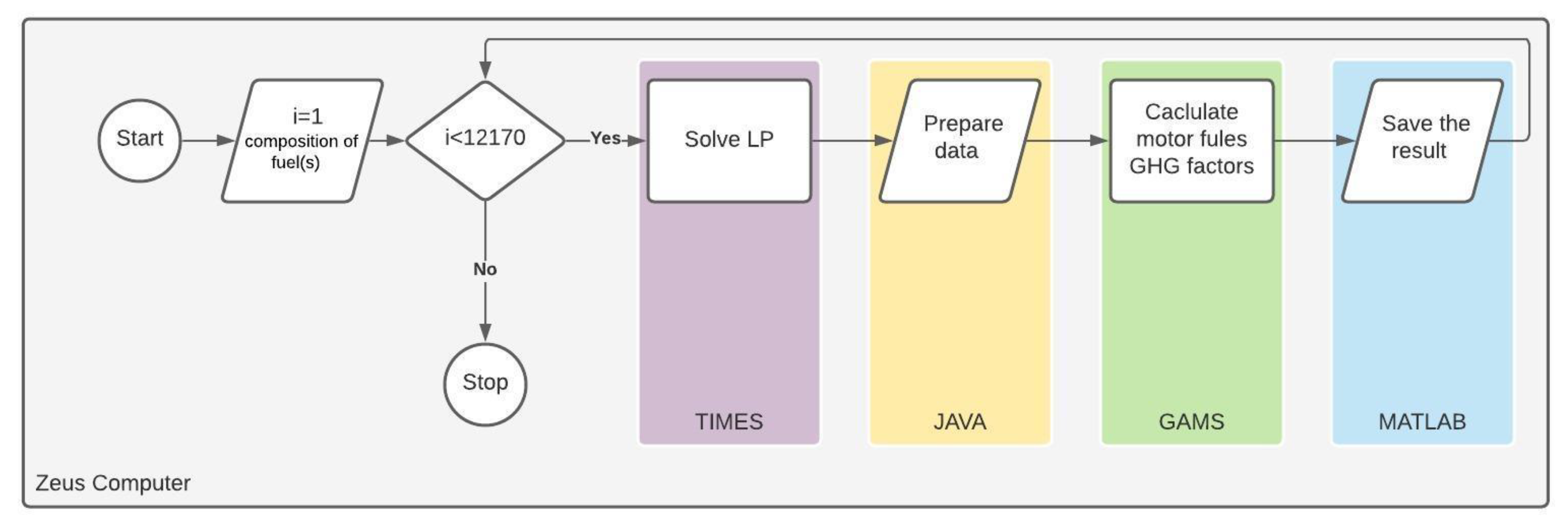
2.5. The Course of the Modelling Work

The modeling work started with the analysis of the reference case for the refinery. In the next step a series of simulations were conducted to determine the refinery settings (fuel component compositions, individual unit loads) yielding the lowest average GHG emissions. Each simulation began by introducing into the model a unique component composition for motor fuels. For such exogenously determined fuel composition, the aim of the model was to search for feasible solutions determining the activities and streams of refinery processes. As a result, a cost-optimal solution was obtained, allowing the production of a given amount of fuels while meeting quality constraints. The results included input and output streams from individual processes. The integral part of this work was the refinery model developed with the use of the TIMES generator. TIMES code was written with the use of General Algebraic Modeling System (GAMS) [42]. It solved a linear programming problem (LP) with the objective function given by equation (1) and set of constrains given by Equations (2)–(10). The constrained optimization was conducted with the use of the CPLEX solver [43]. Additional modules had to be developed for data processing and management (coded in JAVA and MATLAB) as well as for calculating allocation factors of GHG emissions to motor fuels (coded in GAMS). The algorithm for conducting simulations is depicted in Figure 2.

The unique component compositions of the fuels were determined using the modified Anderson and McLean method of experimental planning [44]. For each fuel, the limiting proportions of each component were determined separately, as well as the acceptable limits within which the fuel quality parameters should fall.

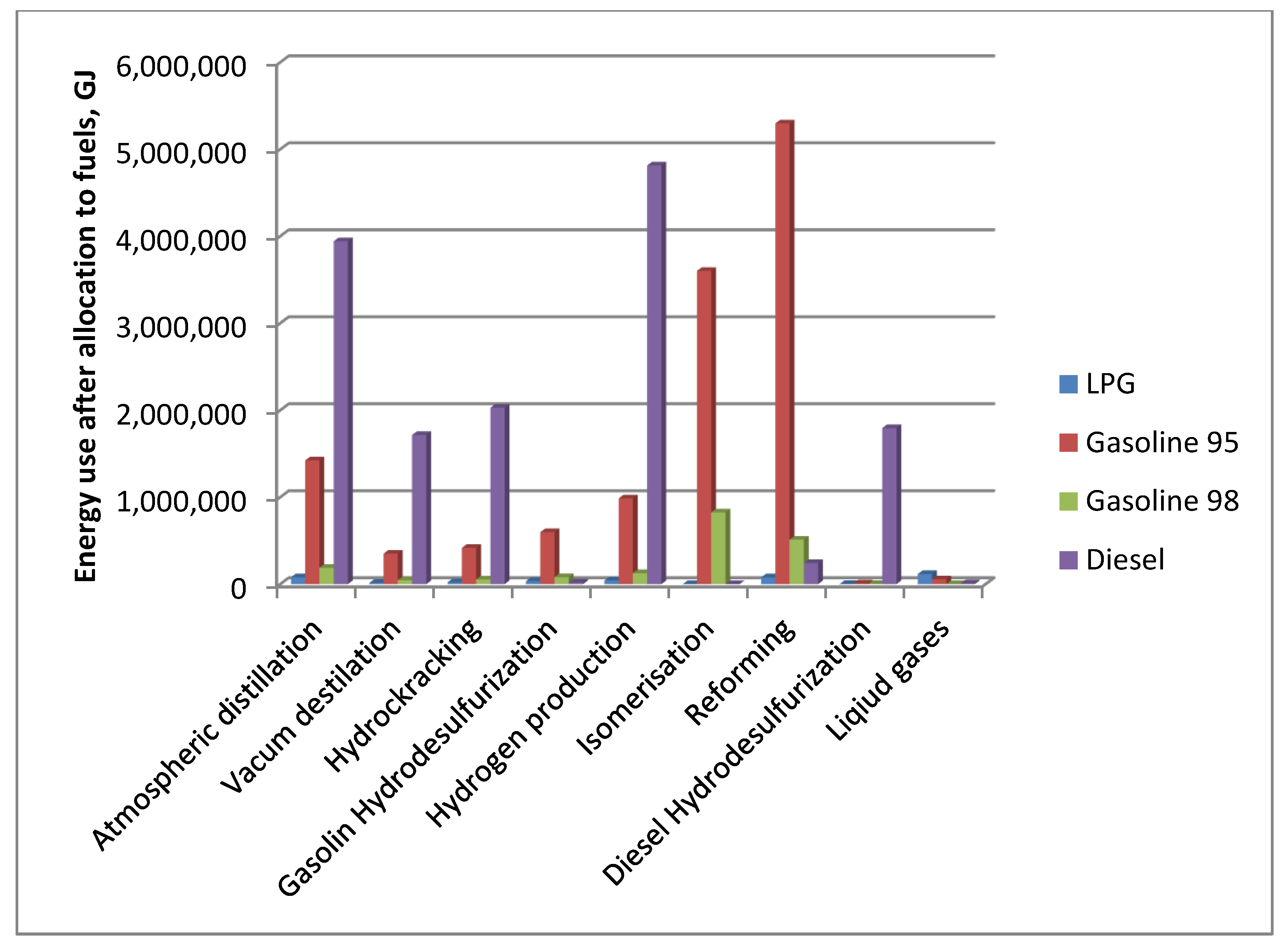
3. Results and Discussion

In each simulation the demand for energy carriers of individual refinery installations varies due to the nature of the installations’ operation. Hence, there is also a difference in GHG emissions allocation factors to motor fuels. The values of energy consumption in processes allocated to motor fuels for the reference case are depicted in Figure 3. The highest values were assigned to the reforming, hydrogen production and atmospheric distillation installations.

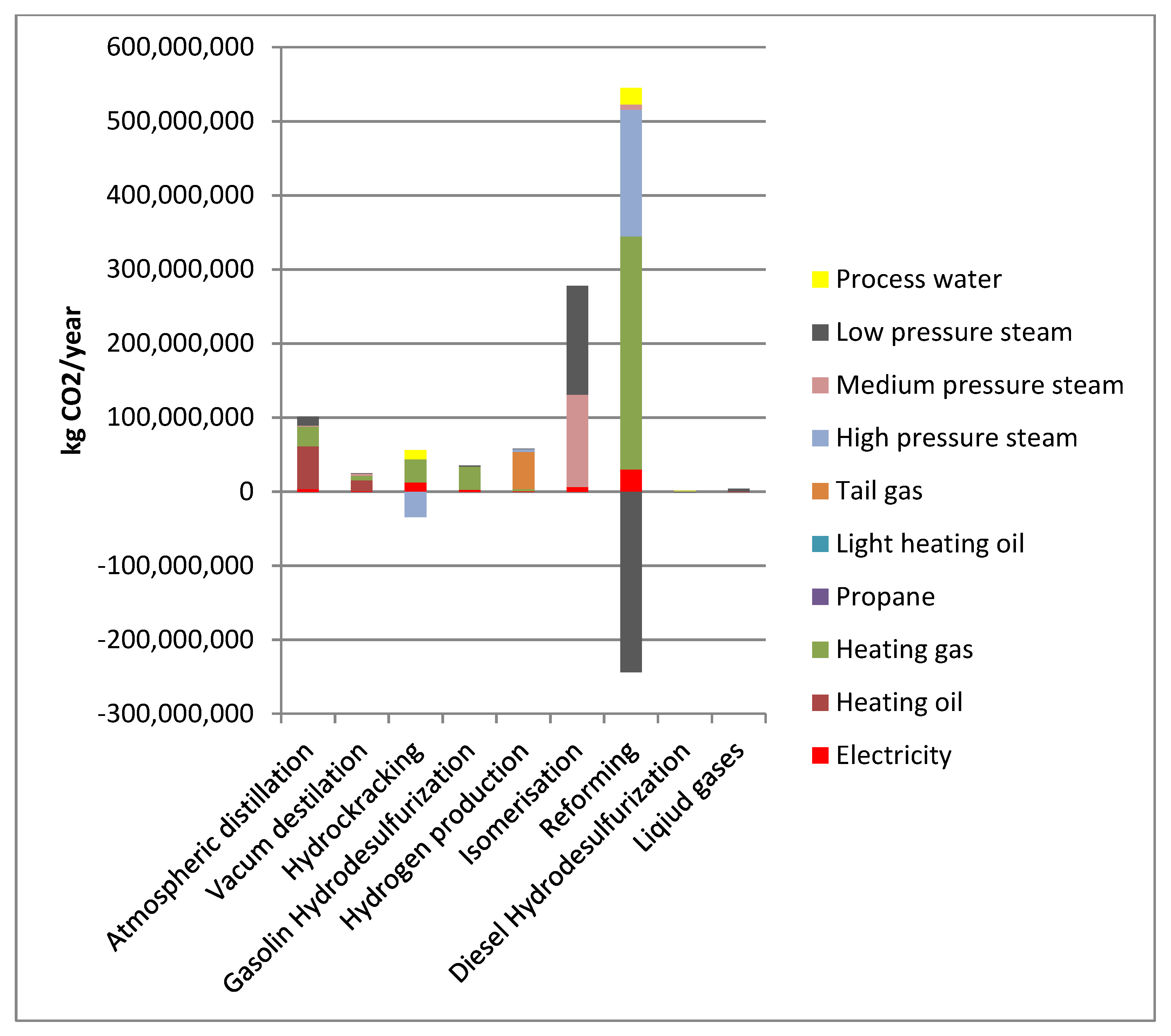
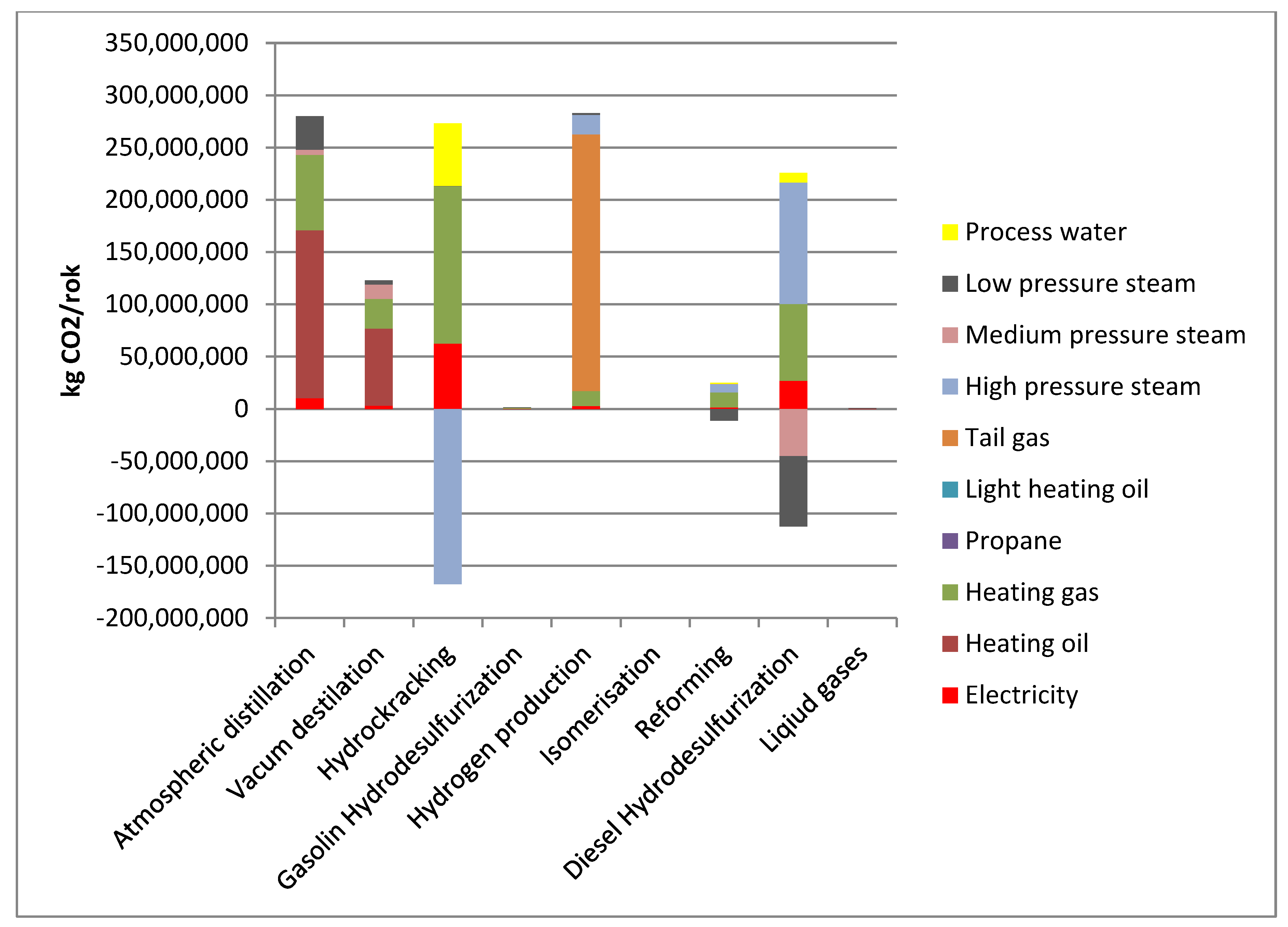
These results were then used to allocate energy and GHG emissions generated by individual processes/installations to motor gasoline 95 as depicted in Figure 4.

Negative GHG emission for the reforming installation is a consequence of the adopted method of accounting for steam generated at the installation. Analysis of the above data indicates that in case of motor gasoline 95, the reforming contributes to the GHG emission to the highest degree. Form the energy carriers point of view, the highest emissions are associated with the technological steam and heating gas. Therefore, the introduction of low-carbon energy sources in these areas will be most effective in reducing GHG emissions for the crude oil processing stage. Figure 5 presents the GHG emissions allocated to diesel fuel.

In the case of diesel, the installations that generate the most GHG emissions are: Atmospheric Distillation, Hydrocracking, Hydrogen Production, and HDS. Among energy carriers: Process steam, heating gas, fuel oil at the Atmospheric Distillation and Vacuum Distillation installations, as well as the tail gas at the Hydrogen Production facility contribute the most to the GHG emissions.

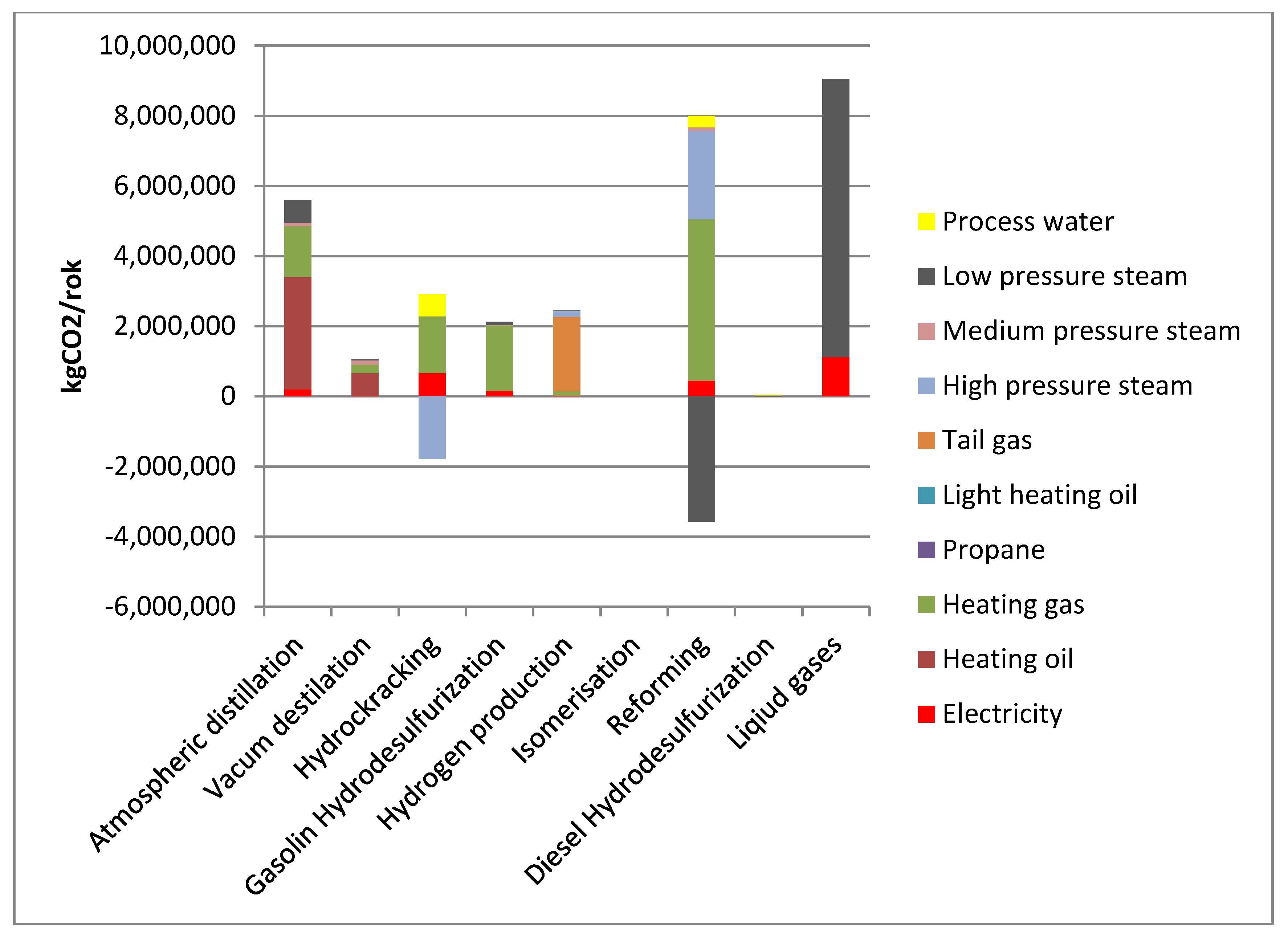
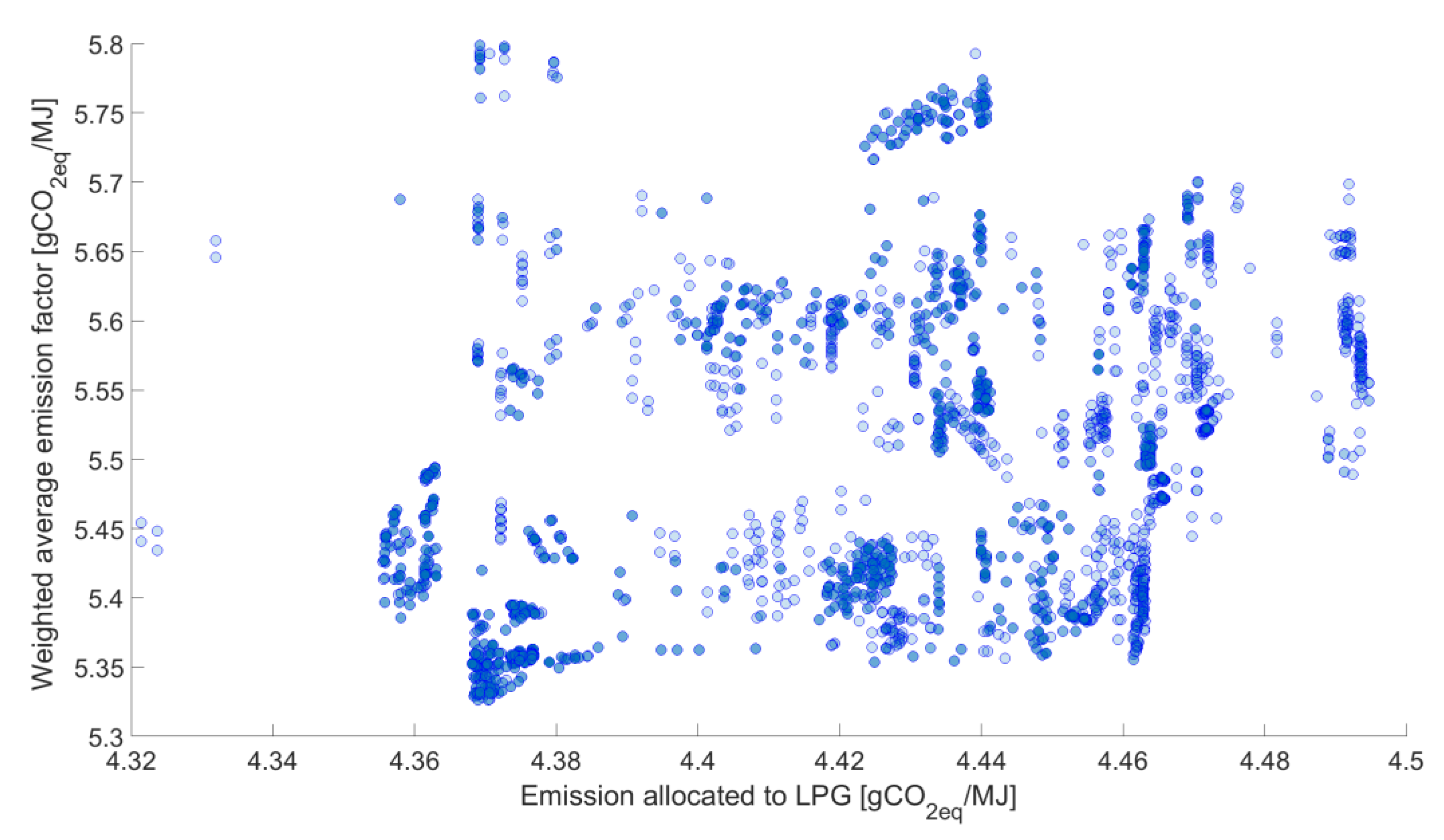
Figure 6 presents the GHG emissions allocated to LPG.

For LPG, the facilities contributing the most to GHG emissions are: the Liquid Gas Unit, Reforming and Atmospheric Distillation through the use of the following energy carriers: Low pressure steam, heating gas and fuel oil.

To sum up, it should be stated that in the reference case the use of energy carriers such as: Process steam, heating gas and in the case of diesel production also tail gas on the hydrogen production installation contributed the most to GHG emissions.

The allocated GHG emissions presented in Figure 4, Figure 5 and Figure 6 represent the annual absolute values. These values should be related to the amount of fuel produced according to the adopted functional unit i.e., gCO₂-eq/MJ of energy contained in a given fuel. For the reference case, using data presented in Table 2 the determined GHG emission factors equaled to: for LPG: 4.40 gCO₂-eq/MJ, for gasoline 95: 8.76 gCO₂-eq/MJ, for gasoline 98: 9.74 gCO₂-eq/MJ and for diesel fuel: 4.19 gCO₂-eq/MJ. The average GHG emission intensity for the refinery stage equaled to 5.70 gCO₂-eq/MJ. It should be noted, that this results consider only the fossil part of motor fuels without biofuel.

A summary of life-cycle GHG emissions from motor fuels in the reference case is provided in

Table 3. Life-cycle GHG emissions from motor fuels in the reference case [gCO₂-eq/MJ].

Energy Carrier	LPG	Gasoline 95	Gasoline 98	ON
Crude oil extraction	7.00	7.00	7.00	7.00
Oil Transportation	0.88	0.88	0.88	0.88
Fuels production in refinery	4.40	8.76	9.74	4.19
Transportation to storage depots	0.16	0.16	0.16	0.16
Storage in fuel depots	0.11	0.11	0.11	0.11
Transportation to petrol stations	0.75	0.75	0.75	0.75
Combustion in cars engines	65.68	73.38	73.38	73.25
Overall	78.98	91.04	92.04	84.17

.

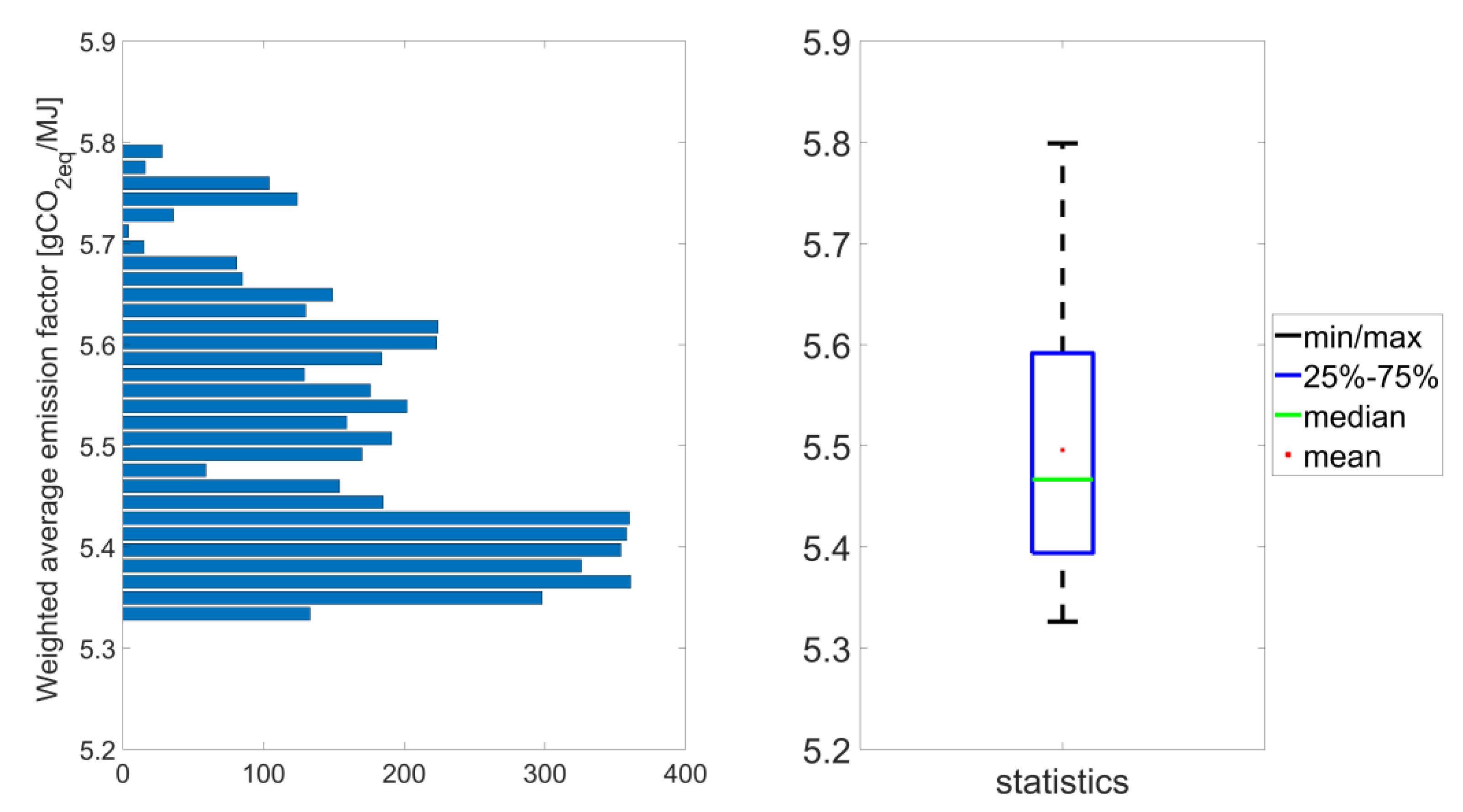
In the next step, a series of simulations were conducted for the crude oil processing level set to 12,435,000 thousand tons, each with the unique component compositions of the fuels to determine the refinery settings yielding the lowest average GHG emissions. More than 5000 feasible refinery arrangements were obtained, which were stored in ca. 600 thousand records. The obtained average GHG emissions ranged from 5.33 gCO₂-eq/MJ to 5.80 gCO₂-eq/MJ as presented in Figure 7. The average value obtained for the reference case (5.70 gCO₂-eq/MJ) is in the upper range of the average GHG emissions obtained as a result of the performed simulations.

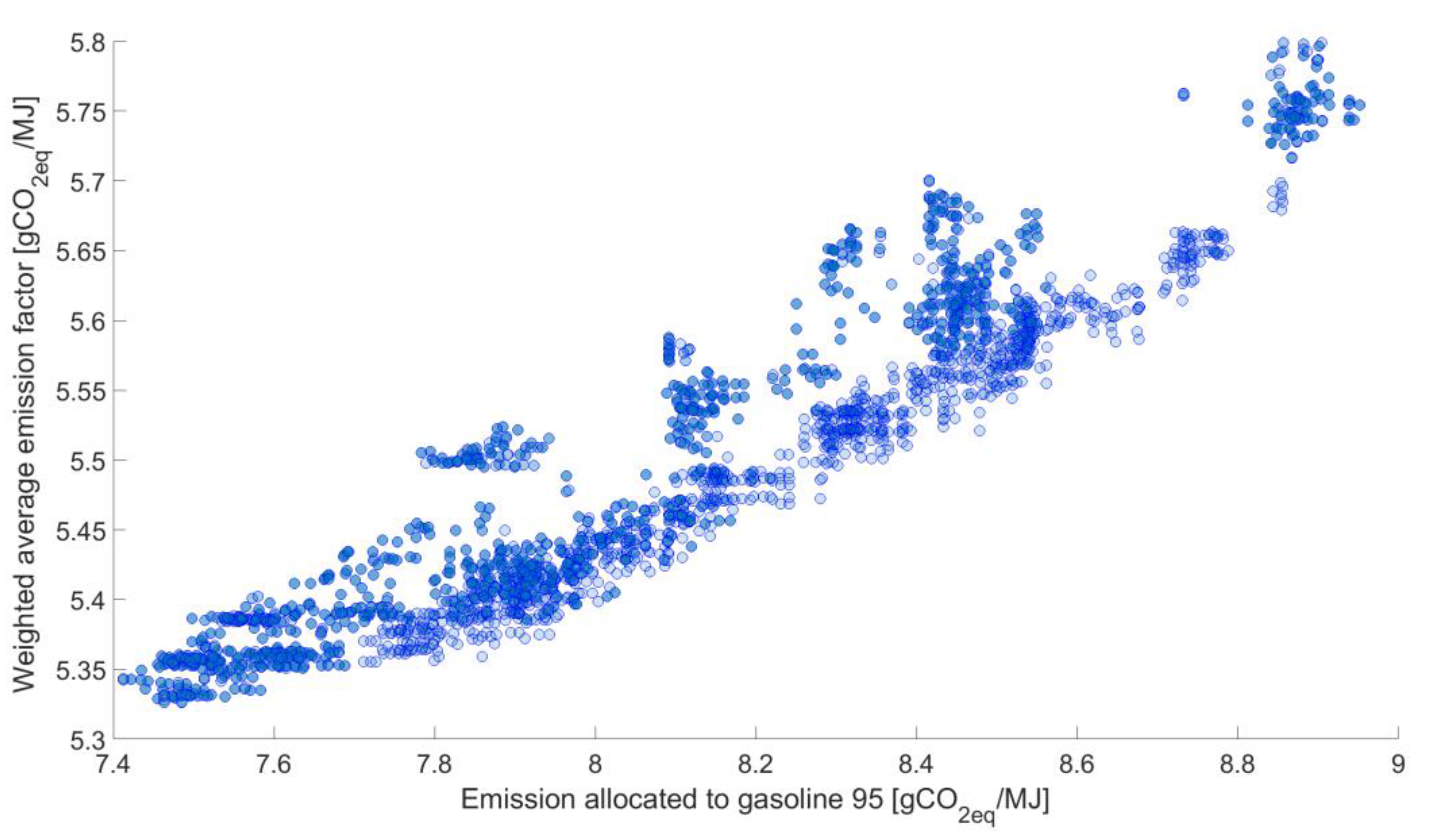
Majority of the obtained values of GHG emissions of motor fuels is lower than the obtained average. Also the median is lower than the mean value. The boundaries of the interval containing from 25% to 75% of the results correspond to the values: 5.4 gCO₂-eq/MJ, and 5.6 gCO₂-eq/MJ, respectively. The minimum and maximum values equal to 5.33 gCO₂-eq/MJ, and 5.80 gCO₂-eq/MJ, respectively. The dependence of the average GHG emissions rate on the GHG emission rate allocated to gasoline 95, LPG, and diesel are graphically illustrated in Figure 8, Figure 9 and Figure 10.

While analyzing the data presented in Figure 8, Figure 9 and Figure 10, it can be clearly seen that there is a correlation between the weighted average and GHG emissions allocated to gasoline 95, with no such clear dependence for LPG and diesel. In the case of diesel, there are clearly shaped groups of results around one value of GHG emissions allocated to this fuel. In order to analyze this phenomenon, the results, highlighted in yellow, were selected. Subsequently, for this set—the dependence is presented in Figure 11 in the three-dimensional system that also considers the emissions allocated to gasoline 95.

The analysis of the data, shown in Figure 11, clearly indicates that the average GHG emissions in the selected set of results, which have the same emissions allocated to the diesel in fact changes in line with the changes in emissions allocated to gasoline 95.

In general, the range of determined GHG emission allocated to diesel varies from 4.088 gCO₂-eq/MJ to 4.3331 gCO₂-eq/MJ. Therefore, the difference between determined minimum and maximum value, i.e., 0.2451 gCO₂-eq/MJ is very narrow for diesel while an analogical difference for gasoline 95 equals to 1.5395 gCO₂-eq/MJ (minimum value is 7.4124 gCO₂-eq/MJ, maximum value is 8.5919 gCO₂-eq/MJ).

Therefore, one may conclude that the weighted average GHG emission factor allocated to motor fuels mostly depends on the GHG emissions allocated to gasoline 95.

In addition, the impact of the use of low-carbon fuel for process heating on GHG emissions was analysed. It has been assumed that heating gas has been entirely replaced by biomethane, while the remaining energy carriers remain unchanged, neither in terms of quantity, nor in terms of GHG emission characteristics. Due to the similar nature of both fuels, it has been assumed that the efficiency of heating devices remains unchanged, thus the amount of this fuel consumed also remains unchanged. It was assumed that the biomethane was produced from bio-waste, using technology with off-gas combustion. For such a biofuel, Directive 2018/2001 gives a typical value for life cycle GHG emissions of 10 gCO₂-eq/MJ. This value that was used for the calculations. The calculations were done for the reference case. The weighted average emission factor of motor fuels after changing the heating gas to biomethane was decreased to 3.66 gCO₂-eq/MJ. The results of the calculations indicate that the use of low-emission boiler fuels is an effective way to reduce GHG emissions over the life cycle of motor fuels. A significant decrease in allocated GHG emissions was observed for gasoline 95 at the reformer installation, as heating gas accounted for a significant proportion of the boiler fuels used there (Figure 4). An apparent decrease in GHG emissions was also observed for the atmospheric distillation and hydrocracking facilities. GHG emission after allocation to gasoline 95 on the isomerization installation remained at a similar level. Therefore, it can be stated that the share of isomerizate will still remain the main factor determining GHG emission rate for motor gasoline. For diesel, reductions in allocated GHG emissions were observed for almost each installation. The largest decrease in GHG emissions was observed for hydrocracking.

Table 4. GHG emissions from motor fuels by sources [gCO₂-eq/MJ].

Source	Gasoline 95	Gasoline 98	LPG	Diesel
Our research	8.76	9.74	4.40	4.19
European Commission, JRC IET [45]	7.00	7.00	-	8.60
Ecoinvent [46]	7.70	7.70	6.90	4.70
Alberta Research Institute [47]	12.50	-	C3: 10.60 C4: 7.40	11.20

shows the results of similar studies in which the energy-based allocation method of GHG emissions to motor fuels was used.

It should be noticed that many factors, such as allocation procedure, refinery scheme, etc. have an impact on the results. Therefore, the observed tendency rather than the exact numbers should be a subject of comparison. Our results were the closets to the ones provided by the Ecoinvent database.

As compared to our study in the JRC work the same order of magnitude was obtained in case of gasoline whereas the emissions allocated to diesel were much higher. According to the Alberta Research Institute diesel fuel is characterised by lower emission factor than gasoline. Such a tendency is also observed in our study.

4. Conclusions

In this paper, a mathematical model of a refinery was developed, using the TIMES model generator with accompanying data processing modules, to analyze the impact of process optimization on GHG emissions at the motor fuels production stage. The model included ten major refinery units, including atmospheric and vacuum distillation, hydrocracking, isomerization, etc., and additionally gasoline, diesel and LPG blending units. The model was tested in the reference case reflecting the real refinery with a simple scheme of crude oil processing.

The modeling work started with the analysis of the reference case for the refinery. In the next step, a series of simulations were conducted to determine the refinery settings (fuel component compositions, individual unit loads) yielding the lowest average GHG emissions allocated to the motor fuels. For exogenously determined fuel compositions, the aim of the model was to search for feasible solutions determining the activities and streams of refinery process. As a result, a cost-optimal solution was obtained, allowing the production of a given amount of fuels while meeting quality constraints. More than 5000 of feasible refinery arrangements were found.

The obtained weighted average GHG emissions allocated to motor fuels ranged from 5.33 gCO₂-eq/MJ to 5.80 gCO₂-eq/MJ, while in the reference case it equaled to 5.70 gCO₂-eq/MJ. It was shown that this weighted average GHG emission factor, allocated to motor fuels, mostly depends on the GHG emissions allocated to gasoline 95. The impact on GHG emissions of the use of low-carbon fuel for process heating was analyzed. The weighted average GHG emission factor of motor fuels after changing the heating gas to biomethane equaled to 3.66 gCO₂-eq/MJ. The results of the calculations indicate that the use of low-emission boiler fuels is an effective way to reduce GHG emissions over the life cycle of motor fuels. A significant decrease in allocated GHG emissions was observed for gasoline 95 at the reformer installation. The study showed that fuel blending management could lead to the reduction of GHG emissions by 0.4 gCO₂-eq/MJ, while the use of low-carbon fuel for process heating results in a reduction of GHG emissions by ca. 2 gCO₂-eq/MJ.

The study covered only two factors, which have an impact on the final GHG emissions in the life cycle of motor fuels, i.e., motor fuels composition and replacement of one energy carrier used for process heating. Findings from this research can improve fuels blending system design and performance by indicating the most effective way of GHG reduction. The results show that using the low-carbon heating fuel is more effective in reducing GHG emission than managing the fuels composition. It should be noticed, that different energy carries are used in refinery installations and their contribution to final GHG emission vary. The effect of using other low carbon energy carriers for process heating should be investigated in future studies. Additionally, the costs of introducing low-carbon heating fuels should be considered.

The developed mathematical model and approach for conducting life cycle GHG emission calculations for the refinery stage can be used to support production management and decision-making processes in refineries.