Abstract
The increasing demand for Electric Vehicle (EV) charging is putting pressure on the power grids and capacities of charging stations. This work focuses on how to use indirect control through price signals to level out the load curve in order to avoid the power consumption from exceeding these capacities. We propose mathematical programming models for the indirect control of EV charging that aim at finding an optimal set of price signals to be sent to the drivers based on price elasticities. The objective is to satisfy the demand for a given price structure, or minimize the curtailment of loads, when there is a shortage of capacity. The key contribution is the use of elasticity matrices through which it is possible to estimate the EV drivers’ reactions to the price signals. As real-world data on relating the elasticity values to the EV driver’s behaviour are currently non-existent, we concentrate on sensitivity analysis to test how different assumptions on elasticities affect the optimal price structure. In particular, we study how market segments of drivers with different elasticities may affect the ability of the operator to both handle a capacity problem and properly satisfy the charging needs.
1. Introduction
Today, the transport sector accounts for a large share of global pollutant emissions. Indeed, in the last few years, the majority of transportation emissions-related health impacts occurred in the top global vehicle markets. In 2015, 70% of transportation-attributable deaths occurred in the four largest vehicle markets: China, India, the European Union (EU), and the United States [1]. As discussed in [2], reducing air pollution from transportation, and especially carbon dioxide emissions, are at the center stage of discussion by the world community. For that reason, over the last decade, there has been a dramatic increase in the number of electric vehicles (EV) in industrialized countries.
The main motivation behind this study is that the large penetration of EV leads to situations where charging puts pressure on the distribution grid. However, the peak loads occur only throughout a small part of the day, while during the rest of the day, the grid has excess capacity. Hence, it is worthwhile to investigate if, utilizing charging flexibility on the demand side to reduce the peak-loads, can be a valid alternative to grid reinforcements within charging sites’ expansion [3]. In the distribution grid, this can be done through demand response, that aims at leveling out the load curve in order to avoid that the power consumption exceeds the grid capacity.
Two types of demand responses exist. With a direct demand response, customers’ loads are controlled by a third party, such as a retailer, or by the DSO; while with an indirect demand response, the customer responds to signals, such as price, that are sent to motivate a certain behaviour that is beneficial for the operator and for the grid [4]. A conceptual introduction to indirect control for demand-side management is proposed in [5].
This study utilizes elasticity matrices in indirect control scheduling models for managing the charging of electric vehicles. The objective is to ensure better utilization of the grid and to reduce the probability of congestion. Assuming that electric vehicle drivers are willing to change their behaviour according to price variations, the paper provides mathematical optimization models to define optimal charging prices. A price list will be created according to drivers’ flexibility and sensitivity to price, in order to reduce their charging in those periods that are critical for the grid because of capacity shortage. The objective is to minimize the curtailment of charging loads by planning load-shifting and, whenever it is not possible to only shift demand, find a solution with minimal curtailment.
Compared to other works in the literature that focus on charging patterns’ optimization, such as [6,7,8,9], the present paper focuses on micro-economics strategies rather than technical properties of the storage technologies. The proposed approach is not about individual pattern optimization. The proposed approach uses an aggregated perspective where customers’ behaviour can be described by elasticity. From this perspective, customers are grouped into clusters that have different sensitivity to prices.
The key contribution of this study is the inclusion of the micro-economic concept of elasticity in the optimization strategy. In particular, the proposed mathematical models will make use of an elasticity matrix to map the driver’s sensitivity to price and forecast their reactions to the price signals in terms of a demand increase or decrease. Although the general concept of elasticity is well-established, its use within the pricing of electric vehicle charging is relatively new. Due to the novelty of this approach, real-world data relating the elasticity values to the electric vehicles’ drivers’ behaviour are currently nonexistent. Hence, beyond the methodological contribution in terms of mathematical modeling, the present paper will provide an analytical contribution in terms of sensitivity analyses and representative case studies aimed at understanding the effect of the elasticity in the pricing of electric vehicles. The proposed mathematical models are used to investigate how elasticity data may affect the pricing, the behaviour of drivers, and the ability of the operator to successfully handle critical periods of capacity shortage.
The rest of the paper is organized as follows. Section 2 will present an overview of previous literature dedicated to control schemes for EV drivers. Section 3 will discuss the main concepts of demand curves and the elasticity matrix in the EV sector, while Section 4 will propose mathematical optimization strategies for indirect scheduling of EV charging with price signals. Computational experiments and sensitivity analyses will be presented in Section 5 and conclusions will be drawn in Section 8.
2. Literature Review
This section aims at providing a short overview of previous literature dealing with how to affect EV drivers decisions in a way that is beneficial for the grid. The main areas are charging scheduling schemes, demand response strategies, and more specifically, the use of microeconomic concepts, such as elasticity to define charging prices.
A survey on economy-driven approaches for charging electric vehicles in the smart city is proposed in [10], where the most common approaches are presented and compared.
An example of indirect control can be found in [11], where a fuzzy logic controller is used to control and manage the charging process in order to maximize electric utility and the electric vehicles’ owner benefits. Another study presented in [12] compares three approaches (heuristic, optimization, and stochastic programming) used to schedule under uncertainty the charging process of three different electric vehicles’ fleets at a common charging infrastructure. Dynamic price signals are developed in [13] to implement demand-side management, and alleviate the stress of concurrent charging on the distribution network. A statistical demand-price model with its application in optimal real-time price is presented in [14], and a similar work is proposed in [15]. Demand response opportunities of EV to improve the reliability of distribution networks are explored in [16]. A stochastic approach to handle uncertainty in price elasticities of electricity demand is proposed in [17]. A price-based approach to prevent distribution grid congestions by integrating indirect control in a hierarchical EV’s management system is developed in [18].
None of the above works include elasticity formulations within mathematical optimization models, to study the price sensitivity of the drivers. As previously outlined, there are no papers that use elasticities within scheduling models for the charging of electric vehicles, which in the same way is proposed in this paper. However, a few papers make use of it in related models and analyses.
The broad concept of real-time price elasticity of electricity has been addressed in [19], where the authors provide a quantification of the real-time relationship between total peak demand and spot market prices. Elasticity theory and its relevance within a scheduling program is presented in [20], but the focus is on general electric load management, and not related to electric vehicles’ management in conditions where there is a lack of capacity. Elasticities are used in [21] to analyse investment decision-making and investigate the propensity to switch from a private car trip to a car-sharing service, as well as the propensity to choose an electric vehicle for such a service. A heuristic method is proposed in [22] to forecast elasticity values, but the main application is households’ electric load management and not indirect control of electric vehicles. A demand response model with elasticity inclusion to handle general electric loads is proposed in [23], but without the objective of defining an optimal set of prices. Indeed, prices are not generated by the model, but rather provided as input parameters within the case studies. Moreover, the study is not directly related to electric vehicle scheduling. Similarly, in [24], the authors make use of an elasticity matrix to develop models for residential demand response. Both [25,26] propose methodologies to handle demand response in systems that include electric vehicles, but their main focus is the possibility to manage the uncertainty by using the renewable resources in the system rather than the electric vehicles and their impact on the available capacity of the grid. The optimal installed capacity allocation of renewable resources in conjunction with demand response is also analysed in [27], where authors do make use of an elasticity matrix to forecast the consumers’ behaviour. The study in [28] proposes a smart-charging management system considering the elastic response of electric vehicle users to the electricity charging price. However, a deeper investigation of the actual sensitivity of elasticity values is not provided. A behavioural modeling of electric vehicles using price elasticities is proposed in [29] to provide insights into the degree of demand-shifting that can occur across various day-ahead electricity market scenarios. An approach to model demand flexibility of electric vehicles is proposed in [30], where the demand flexibility offered by an EV is represented using a price elasticity matrix which is calculated with respect to a flat reference price scenario. However, the work does not provide enough insights into the value of an elasticity matrix due to the lack of elasticity data.
A methodology for an optimal operation and bidding strategy of a Virtual Power Plant integrated with energy storage and an elasticity-based demand response is presented in [31]. The price elasticity of consumers is also taken into account in [32], where the objective is the development of a decentralized robust model for optimal operation of distribution companies with private micro-grids. An optimal real-time pricing of electricity based on demand response is tested in [33] to encourage customers to participate in the electricity market operation.
One of the challenges in all of the above papers that include elasticities in real-world applications for energy systems, is the lack of actual elasticity data. Additionally, no sensitivity analyses are performed to actually show what is the impact of including an elasticity matrix within the proposed optimization models. Most of the papers propose the use of elasticity values, but they do not provide a thorough investigation of the elasticity impact on the pricing strategies and on the models’ results. There is a need to gain a better understanding of the impact that such elasticity data would have within specific optimization models, and how heavily such values would affect the final results and decisions.
While indirect control in pricing has been used already in the past for demand management, the price elasticity has not been combined together with indirect control strategies in ways suitable for inclusion within real-time decision-making tools based on optimization within the green transportation sector. In addition, while the concept of pricing in a certain time-period is well-established (self-elasticity), the concept of switching between time-periods through price sensitivity (cross-elasticity) has not been fully investigated in the literature, especially for the particular application of electric vehicle charging scheduling. The cross-elasticity of demand is an economic concept that measures the responsiveness in the quantity demanded of one commodity when the price for another commodity changes. The proposed work identifies charging time as a commodity for real-time decision-making processes, where different time-periods are regarded as different alternative commodities, and where drivers are aggregated into segments with different sensitivities to the charging price in different time-periods.
Therefore, the key contribution of the proposed study is to combine indirect control together with price elasticities and check the insights that can be gathered through sensitivity analyses. From this point of view, the key contribution of the present paper is not only proposing a methodology to define optimal price lists to send to electric vehicles’ drivers in order to better manage critical periods of a lack of capacity in the grid, but also performing sensitivity analyses with an in-depth investigation of how the elasticity values would affect the pricing and the ability of the system to fulfill the demand requirements.
The main purpose of the study is to discuss what kind of insight can be gathered by using elasticity within mathematical optimization models for indirect control of electric vehicle charging. Therefore, the focus is on demonstrating the use of elasticity for this specific application, and understanding the value of using elasticity in analysing the outcome of a real-time decision-making process.
3. Demand Curves in the Electric Vehicles Sector
The relationship between the demand of a good and its price is represented with a demand curve. Normally, the demand for goods decreases as the price of the good increases. However, there is also a relation to the price of so-called “substitute goods” that consumers consider as similar or comparable, meaning that demand is reduced if the price of a substitute good decreases.
For EV charging, the demand curve represents the relationship between the charging price of electric vehicles and the amount of drivers that are willing to charge at a certain price in a certain time-step. The substitute goods can be described as the possibility to shift the load and charge in a time-step that is different from the desired one because the related charging price potentially is lower. This study proposes a stylized approach in order to study how elasticities can be used to understand the effect that prices have in order to move demand between time-periods. For the purposes of demonstrating the concept, we simplify the charging scheduling problem to depend only on price. Such simplification is reasonable, since we do not refer to individual drivers, but rather to the aggregated markets’ demand curves. The main purpose of this work is to show how elasticities can be used to better understand the effects that price have on shifting demand between time-periods. In sum, as shown in Formula (1), the charging demand of electric vehicles is a function of both the price in a certain time-step t and the price that the operator shows in alternative time-steps ().
Moreover, it is important to note that when analysing consumers’ response to price, the focus is generally not on the single consumer demand, but on the aggregated demand curve stemming from aggregating the demand curves of individual consumers. As a first approximation, it is possible to consider one whole aggregated demand curve for charging, aggregating all the electric vehicles’ drivers. As an extension, it is possible to imagine market segmentation, that aims at aggregating the electric vehicles’ drivers into groups, or segments, where drivers within a group respond similarly to a market action (i.e., price change).
Aggregated Demand Curves within Multiperiod Optimiztion Models
It is difficult, if not impossible, to quantify exactly a real non-linear demand curve that is a function of several prices and that involves consideration of prices in different time-steps. Still, using Taylor’s first-order approximation theorem, we know that a multivariate function, that is, can be approximated linearly in the neighborhood of the point of evaluation as:
where denotes the partial derivative of the function with respect to x and similarly for y. The same approximation can be easily extended if f is a function of more than two variables. This can be used to approximate the demand function showed in Equation (1), where demand is a function of different prices in different time-steps. Hence, through the Taylor’s theorem, we are now moving into a description of demand based on point-price elasticity.
The standard definition of elasticity is shown in Formula (3). In this formula, is the partial derivative of the quantity demanded taken with respect to the price, is a specific price for the good, and is the quantity demanded at the price .
In order to include this concept within mathematical optimization models, the standard formulation can be approximated, as shown in Formula (4), where the elasticity is defined as the ratio of the percentage change in quantity to the percentage change in price.
Within the electric vehicle charging sector, two types of elasticities can be identified, the self-elasticity and the cross-time elasticity.
The self-elasticity defines the percentage change in demand Q at time-step t, due to the corresponding percentage change in the price P, at the same time-step t. It has a negative sign, meaning that an increase of price in a certain time-step will cause a decrease of demand in the same time-step.
The cross-time elasticity describes the percentage change in demand Q at time-step t due to a change in price at a different time-step . It has a positive sign, meaning that an increase of price in a certain time-step t can cause an increase of demand in a different time-step .
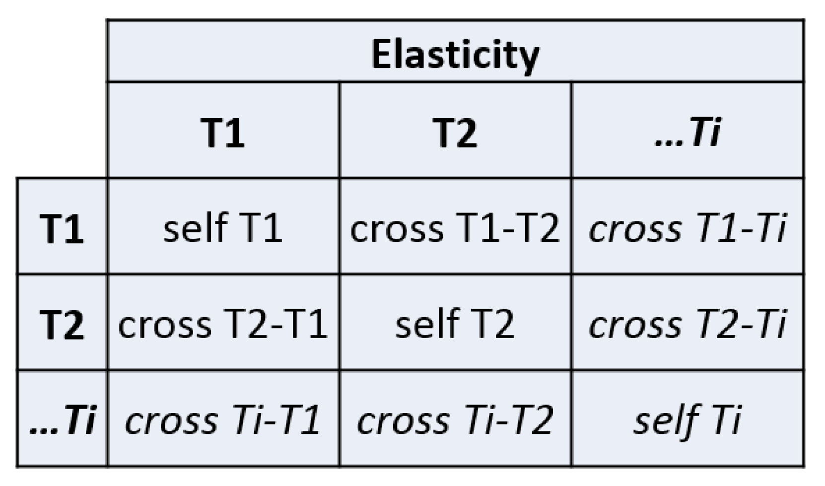
As shown in Figure 1, such elasticity values can be summarized into matrices that give us a quick view of consumers’ sensitivity to prices in different time-steps. Hence, we will no more rely on an exact demand function, but rather on a mapping of drivers’ flexibility, expressed by elasticities and applied to a first-order Tailor approximation.
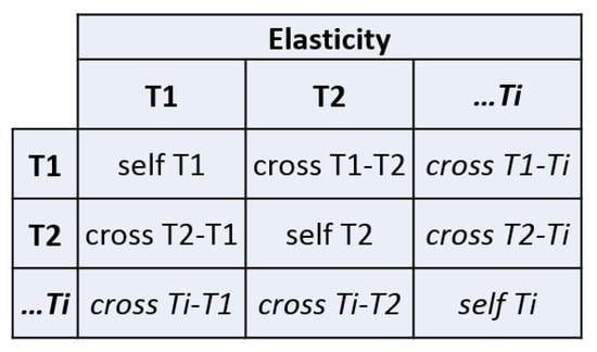
Figure 1.
Example of elasticity matrix with self- and cross-elasticity values.
Here, it is important to remember that the elasticity is a concept to be applied to large groups of users. It does not represent a single driver’s behaviour, but rather the behaviour of a group of drivers that belong to the same market segment and respond similarly to a market action like price variation. We will refer to a group of drivers as a . The idea behind the mathematical model that will be proposed later, is that when a price signal is sent to a group of drivers, some of them will be discouraged and give up the charging, while others will still decide to connect. The objective of the pricing scheme is to shift a portion of drivers in such a way that the capacity limit is respected.
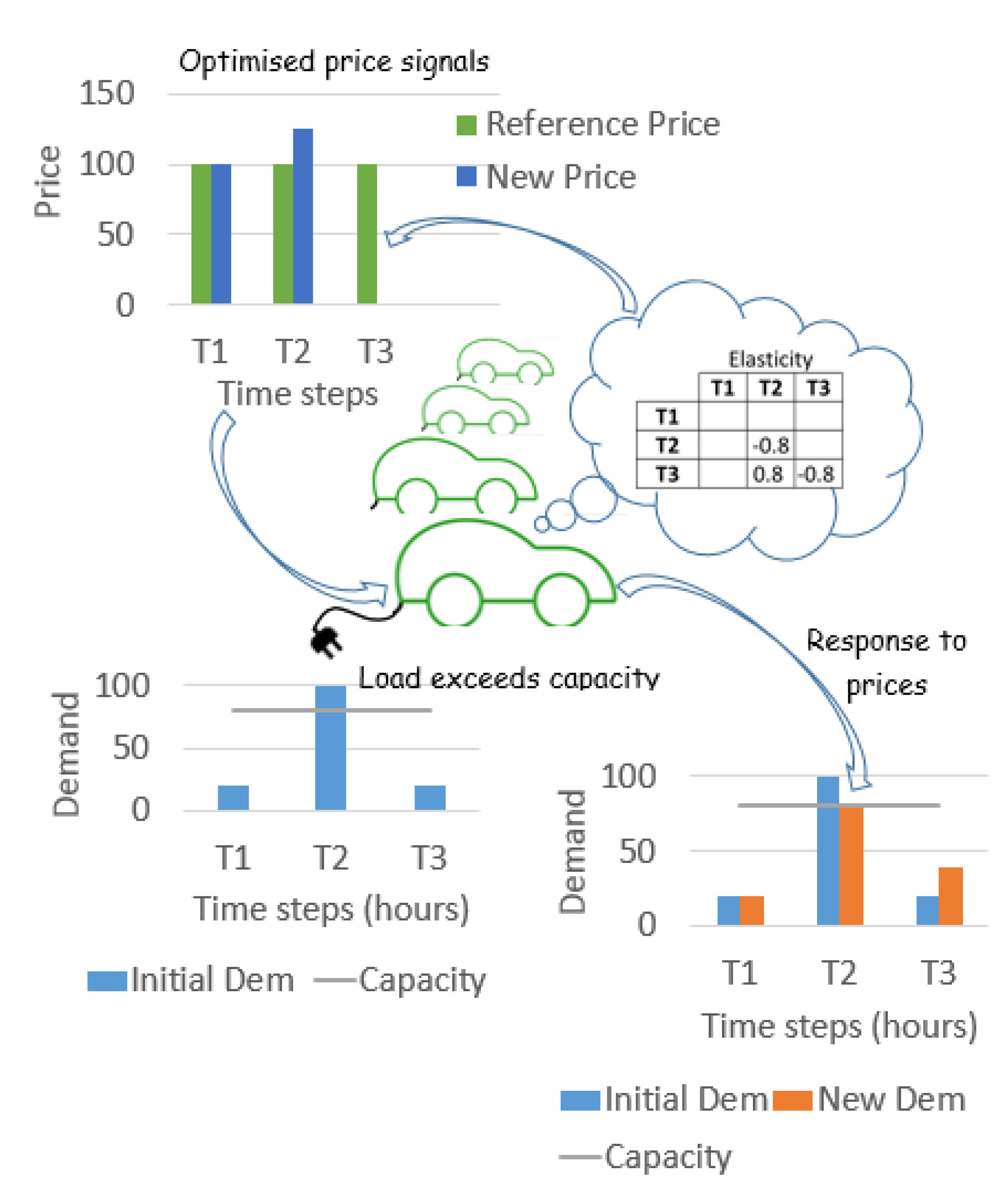
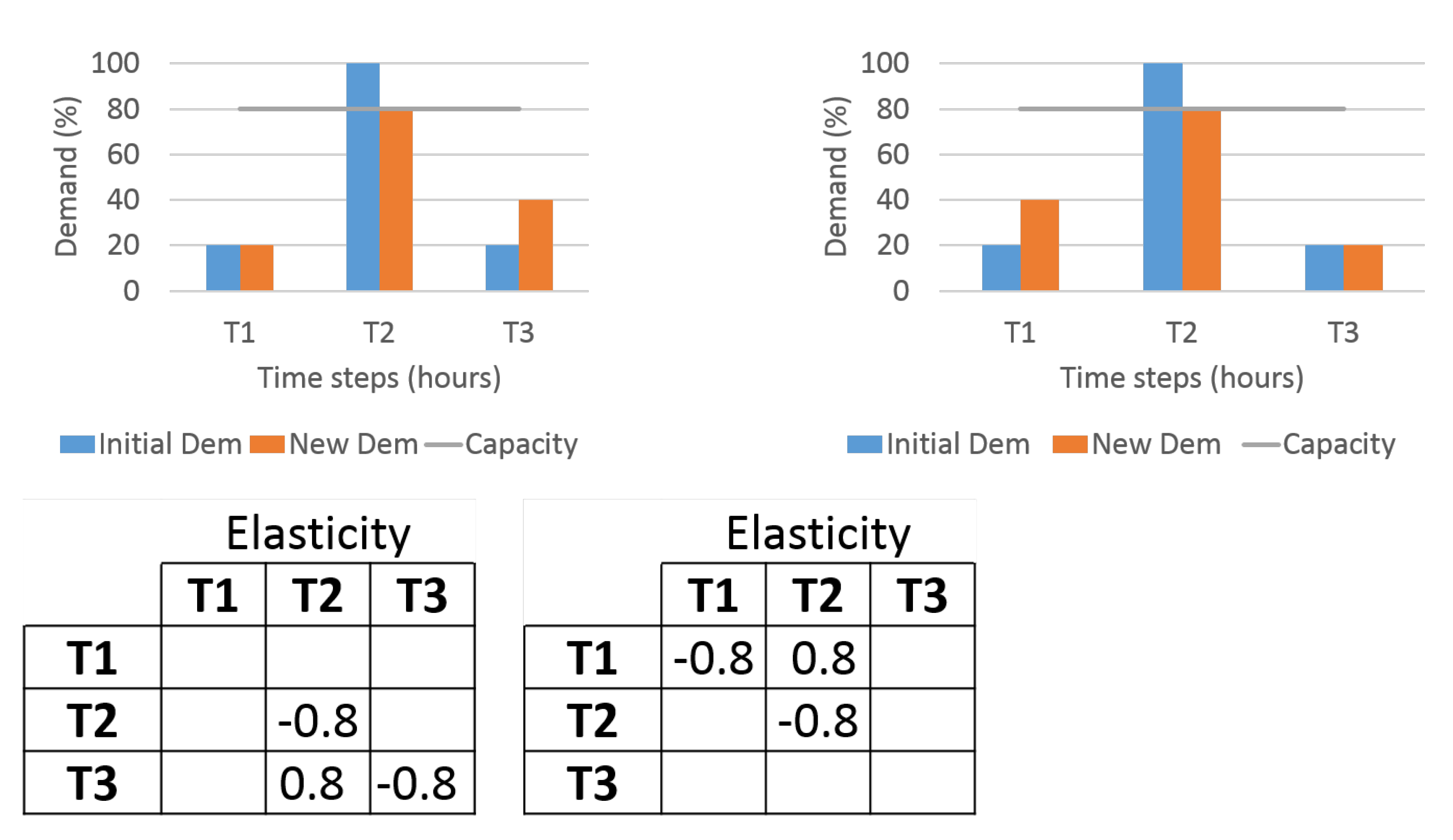
Figure 2 shows the basic idea behind the pricing models. Figure 3 shows a simple example. In time-step , there is a load that exceeds the capacity and that has to be reduced. Therefore, the objective is to send a price signal that motivates the shifting of the exceeding load in or . The elasticity tells us how sensitive a cluster of drivers is. The elements on the diagonal represent the self-elasticity: in this particular example, we assume we increase the price in to get a decrease of demand in , and we decrease the price in or to get an increase of demand in or . Elements above or below the diagonal represent the cross-elasticity. On the left diagram of Figure 3, there is a cross-elasticity below the diagonal, that represents the variation of the demand in due to a change in price in . Therefore, an increase of price in will not only cause a reduction of demand in , but it will also motivate a demand increase in ; hence, part or all the load that has been cut in can be shifted in as a function of the cross-time elasticity of drivers. On the right diagram of Figure 3, there is a cross-elasticity above the diagonal, that represents the variation of demand in due to a variation of price in . Therefore, for that group of drivers, an increase of price in not only causes a reduction of demand in , but it will also motivate a demand increase in , hence part or all the load that has been cut in can be shifted in as a function of the cross-time elasticity of drivers. When only one market segment is involved, such load movements in time are easy to handle. However, when more market segments with different sensitivities react to the same price signal, then a model is needed to define the optimal price in order to shift the total load while taking into account the different reactions of different clusters. The next section will discuss a mathematical optimization approach for that purpose.
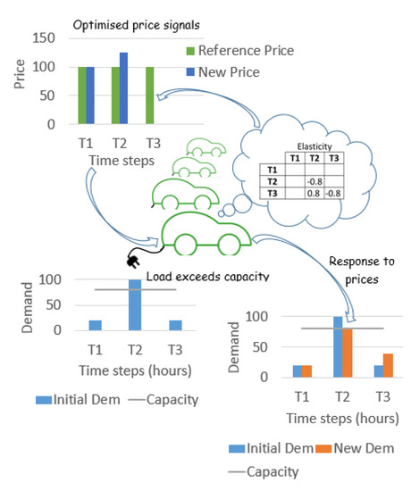
Figure 2.
Graphical representation of the basic idea behind pricing models that make use of the elasticity concept to handle electric vehicle charging needs.

Figure 3.
Simple example to understand how the elasticity affects the loads’ cut and shifting.
4. A Mathematical Model for Indirect Scheduling with Price Signals
This section proposes a mathematical model for indirect control of electric vehicle charging through smart price signals, based on the variables and parameters illustrated in Table 1.

Table 1.
Nomenclature list.
There exist different clusters of EV drivers with different preferences (for example, speed of charging) that are represented as market segments, each with their own aggregated demand curve. We will propose a first basic model that provides a single price list with one price per time-step t. Then, we propose a model extension that generates separate price lists for two different charging speeds (fast or slow charging). Please note that there is no price discrimination between the market segments. The segments just represent different preferences reflected by the elasticities.
4.1. Different Aggregated Demand Segments and Real-Time Price List
In the first basic model for the indirect control of the charging of electric vehicles, the objective is to define an optimal price list to motivate drivers to reduce the charging demand in those time-steps where the total load exceeds the capacity, and increase the charging demand in those time-steps where an excess of capacity is available. Drivers’ sensitivity to price will be mapped according to their elasticity coefficients.
The objective function (5) minimises the difference between the total initial forecasted demand for the chosen time horizon T and the total new demand that will result after reducing load in critical time-steps and increasing the loads in non-critical time-steps. Critical time-steps are those where the total initial demand is greater than the available capacity , while non-critical time-steps are those where there is space for load increase.
Constraint (6) defines the new demand in non-critical time-steps that is not allowed to exceed the available capacity. While constraint (7) defines the new demand in critical time-steps, that is setting it equal to the available capacity. That means the model is forced to find the optimal price signal to cut only the exceeding load, in order to exploit all the available capacity.
Constraint (8) imposes that the total new demand summarized over the defined time horizon T should not exceed the total original demand. That means the model is only allowed to cut and shift loads without creating new additional demand.
The elasticity concept outlined in Formula (3) is integrated in constraint (9) where the demand variation in every time-step is calculated according to the price variation and the elasticity for each of the market segments.
It is important to note that in order to use the concept of elasticity to forecast demand and price variations, we need to define a “reference price" and a “reference demand”, which will represent the first term of the right-hand side of the proposed constraint (9). That is because the elasticity defines the increase and decrease of demand related to a small change in price. The reference price can, for example, be a market price that would occur in a normal situation where there is no congestion. The reference demand can be set as the original initial aggregated forecast demand of the market segments.
4.2. Discussion Potential Model Extensions
The model proposed in the previous section can be further extended to include different features that may be of interest for different real-world purposes. Two main additional features will be briefly introduced below, with regard to price discrimination based on membership, and different pricing for fast- and slow-charging modes.
4.2.1. Price Discrimination Based on Membership
Assuming a certain number of demand segments, may have a membership card, and it is possible to send different price signals to different subsets of demand segments, so that membership card holders can receive a better price compared to other segments that do not hold a membership.
In order to include such a feature, the demand segments can be split into two subsets, namely: segments with are those that have a membership card; segments with are those that do not have a membership card.
For this purpose, the index h should be added to the price variable and parameter, since the price signal is now dependent not only on the time t, but also on the segment h.
Then, two new price parameters should be included: and defining the minimum and maximum price allowed in every time-step t for different demand segments h based on membership.
Two price constraints should be added as follows, such that different price ranges will be allowed for members and non-members:
Different membership levels can also be considered, by further splitting the demand segments into more subsets (i.e., silver, or gold membership that would allow different price benefits).
4.2.2. Different Pricing for Fast-Charging and Slow-Charging
Progressive tariffs can also be included, in order to send different price signals based on the charging speed preferences of the different market segments. A progressive tariff can act as an incentive for the drivers to charge their electric vehicles with a lower power. With a progressive energy tariff, the price per kWh per time-period will be lower for consumers with a normal charging, than for consumers which use fast charging. This provides another mechanism to manage capacity shortage. In addition to smoothing out consumption, this tariff has another benefit. It ensures a more fair distribution of costs among drivers, as only the drivers with a high power consumption should pay more per kWh, while the drivers with a low power consumption do not have to pay more per kWh, as they are not the ones contributing the most to congestion.
One natural extension would be to introduce different price signals for different types of charging (i.e., slow charging and fast charging) with substitution elasticities between them. Slow charging can, for instance, be regarded as up to 4 kWh/h, while fast charging is the amount of charging power exceeding this limit. Further extensions can include a wider variety of charging type requests according to the amount of demanded power per unit of time. For instance, slow charging, fast charging, and rapid charging may correspond to 7.4, 22 and 50 kW, respectively.
In order to include such a feature, it is possible to create different demand segments for fast charging and slow charging. Therefore, the demand and price parameters and variables, as well as the elasticity parameters, can each be split into “fast” and “slow”, namely, , , , , , , , .
The constraint defining the demand variations according to the price (constraint (9)) can be split accordingly, for fast and slow charging, in particular:
- The demand for fast charging now, depends on the fast charging price now, and the fast charging price in the future;
- The demand for slow charging now, depends on the slow charging price now, and the slow charging price in the future.
Moreover, the constraint defining the demand variations according to the price (constraint (9)) can also be split and changed, in order to describe the substitution effect between slow and fast charging, in particular:
- The demand for fast charging now, depends on the fast charging price now, and the slow charging price in the future;
- The demand for slow charging now, depends on the slow charging price now, and the fast charging price in the future.
While in the previous models, the capacity was mainly assumed as the grid capacity, in this new model, extension can be defined either as the grid capacity, or the charging capacity (combination of fast and slow charging availability).
A new constraint can also be included defining as the minimum between the grid capacity and the charging capacity.
5. Computational Experiments and Sensitivity Analyses
5.1. Introduction to the Case Studies
While elasticises are routinely calculated in a number of areas, the research literature on EV-charging has had little focus on them, and as a result, no empirical studies also exist. In our case study, we therefore focus on sensitivity analyses illustrating the effect that different values of the elasticities will have on the scheduling. We provide some basic case studies to investigate the effect of the elasticity concept within the indirect control of electric vehicles. We are particularly interested in investigating how the elasticity affects the price, the forecast behaviour of drivers, and the ability of the operator to successfully handle critical periods of capacity shortage. In sub-cases with different demand segments, we aim at understanding how the elasticity matrix of different segments affect the solution, how they interact, and how the combination of different matrices affect the pricing and the demand reactions. We investigate only the situation with one charging quality.
5.2. Case Studies with One Aggregated Demand Segment
The basic case study with one aggregated demand segment is shown in Figure 4. We consider a basic sub-case of two time-steps and . In we assume a total demand D that exceeds the available capacity C, while lower demand is assumed in . The model will therefore cut loads in and increase loads in according to different self- and cross-elasticity values in an elasticity matrix like the one shown in Figure 4.
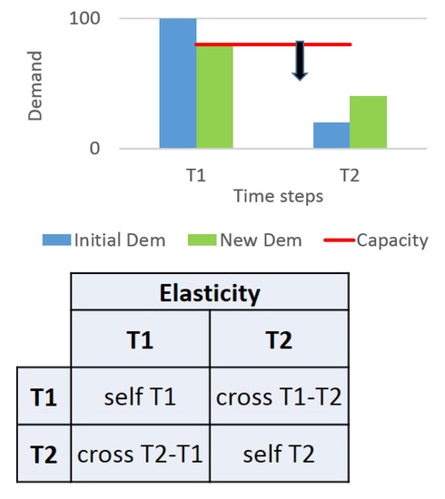
Figure 4.
Graphical representation of the basic case study for the sensitivity analyses.
In particular, looking at Figure 4, the value in the cell defines the self-elasticity in (variation of demand in as a result of a variation of price in ), the value in the cell defines the self-elasticity in (variation of price in as a result of a variation of price in ), the value in the cell defines the cross-elasticity (variation of demand in as a result of a change of price in ), and the value in the cell defines another cross-elasticity (variation of demand in as a result of a change of price in ).
Price signals will be sent to (increasing the price to cut the load) and to (decreasing the price to motivate load increase in this time-step). The price in will be allowed to drop to zero. No minimum price will be set in order to observe the model behaviour without lower bounds that may hide some relevant price-signal variations in .
We will vary the ratio capacity/demand C/D and the elasticity values in order to create patterns and trends that will show the elasticity effects on prices and load variations. The objective is to investigate how the different self- and cross-elasticity values affect the pricing and the ability of the system to manage critical periods.
When studying price signals, it is also worthwhile to make a comparison between the charging price and the price of an alternative diesel solution to see if and when the pricing of electric vehicles is going to be competitive with a traditional combustion engine vehicle. In order to compare the charging cost of an electric vehicle and the cost of filling a traditional diesel vehicle, we calculate the cost per km. The analyses are based on Norwegian cases. Hence, the prices will be given in Norwegian Krones (kr).
The reference price of charging at home is 1kr (100 øre). We assume that an average vehicle requires 1.7 kWh to make 10 km, that means that a realistic cost per km of a home-charged electric vehicle can be assumed to be 17 øre/km.
As for a diesel vehicle, the cost per liter in Norway is set on 1200 øre/liter. We assume that an average vehicle requires 0.7 L to make 10 km. Therefore, a realistic cost per km of a diesel vehicle can be assumed as 84 øre/km. The proposed approximation is suitable to get a preliminary idea of cost levels.
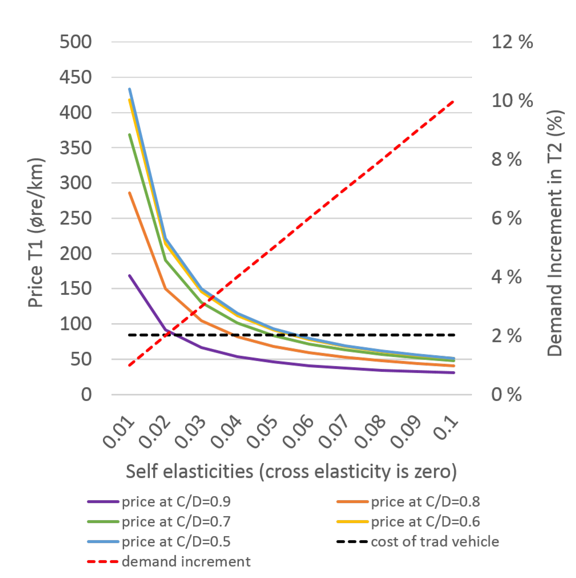
5.3. Case Study 5.01—Effect of Self-Elasticity on the Price and Comparison with a Diesel Vehicle
The main objective of this case study is to analyse the price signal in that is necessary to cut the load to match capacity. The other objective is making a comparison with the cost of filing a traditional diesel vehicle in order to see in which elasticity range the pricing of electric vehicles can still be competitive. For that purpose, we run the model with different ratios’ capacity/demand (C/D) and by varying only the self-elasticities while keeping the cross-elasticities to zero. In practice, that means that there is no willingness to move demand in time, but demand is price-dependent. Figure 5 shows the results.
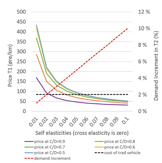
Figure 5.
Effect of the self-elasticity on the price increase in time-step and comparison with the cost of a traditional diesel vehicle.
The curves show that as the self-elasticity in increases, the users become more sensitive to the price, and therefore a lower price change can be used to cut the same amount of load as compared to a low elasticity. Therefore, for every single curve, the required price in decreases as the self-elasticity in increases.
Within every curve, a constant value of the ratio capacity/demand (C/D) is kept. Looking at all the curves together, as the ratio C/D decreases, more loads have to be cut in , and therefore a higher price signal has to be sent. This can be noted watching the curves that are shifted up for higher values of C/D.
The red line shows the linear load increase in according to the price decrease in . Note that no cross-elasticity has been considered so far.
The black line represents the cost of a traditional diesel vehicle and it gives a preliminary idea of how and when the pricing of electric vehicles are competitive with the alternative use of a traditional diesel car—in particular, it is possible to see which combinations of C/D and self-elasticity values are below the curve and are therefore still competitive.
It is important to note that comparing the price of charging an electric vehicle with the current cost of the fuel for a traditional vehicle, does not mean that charging at a higher cost than diesel is not feasible in the short-term.
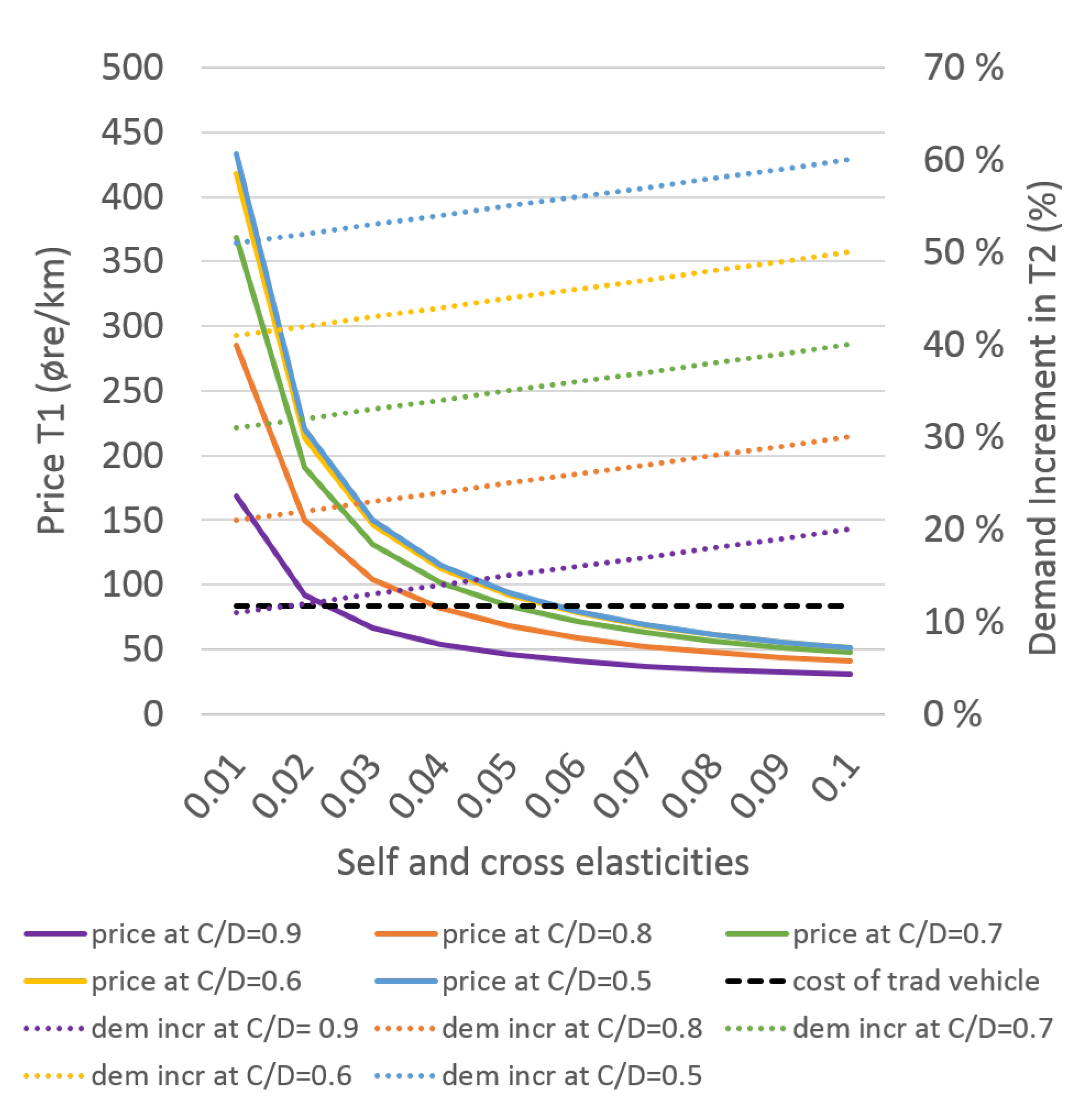
5.4. Case Study 5.02—Effect of Cross-Elasticity - on the Load-Shifting
The objective of this case study is to observe the effect of the cross-elasticities on the loads in time-step and make a comparison for different sub-cases with different ratios of capacity/demand (C/D).
Figure 6 shows the results. Looking at every single dotted line, it can be observed that as the cross-elasticity increases, the effect on load in time increases, as well as a response to a price increase in . Every dotted line represents a constant value of the ratio C/D. Looking at all the dotted lines together, we see that as the ratio C/D decreases, a higher amount of load has to be cut, meaning that the price signal in has to be higher. Per definition, the cross-elasticity defines the variation of the demand in as a function of the variation of price in , hence a price signal in works better the lower the C/D ratio is. This can be noted from the different dotted lines that correspond to different C/D ratios and that are shifted up as the ratio C/D decreases. A lower C/D ratio means that the amount of demand D that exceeds the capacity C is very high. Hence, the lower the C/D ratio, the higher is the amount of demand that exceeds the capacity. This implies that the amount of demand that has to be cut is higher; therefore, the price that has to be sent in order to shift the demand is higher too. The reader will observe a higher demand shifted in , if the ratio C/D is lower, because a higher cut must be done in in order to bring the demand back within the available capacity limits.
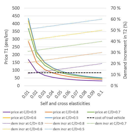
Figure 6.
Effect of the cross-elasticity on the load-shifting.
The price signals work better when cross-elasticities’ effects add on top of the self elasticities’ effects. Indeed, compared to the previous example where only self-elasticity was considered, here the demand increase is higher, because the cross-elasticity effect is summing over the self-elasticity effect.
6. Case Studies with Two Aggregated Demand Segments
This section discusses case studies where two clusters of drivers are considered. The objective is to show how market segments with different elasticities can be utilized when exposed to the same price signal. Three different case studies are presented in order to illustrate relevant interactions between different elasticity values and pricing. Hence, the data have been chosen for illustration purposes only, as no real-world elasticity data for the electric vehicles field are available at the current state of the knowledge.
6.1. Case Study 6.01
In this first case study, we analyse the influence that clusters with different self-elasticity have on the price signals and how they interact.
Table 2 represents a basic sub-case where the whole demand in time-steps and belong to segment number 1. To the left, the table shows the input data (available capacity, reference price, and initial demand in every time-step) and the results obtained after the optimization to the right (new forecasted demand and new price in every time-step for the two demand segments considered). The lower part of the table shows the elasticity matrix for the demand segments.
Table 2.
Case Study 6.01—basic sub-case, data, and results.
Table 2.
Case Study 6.01—basic sub-case, data, and results.
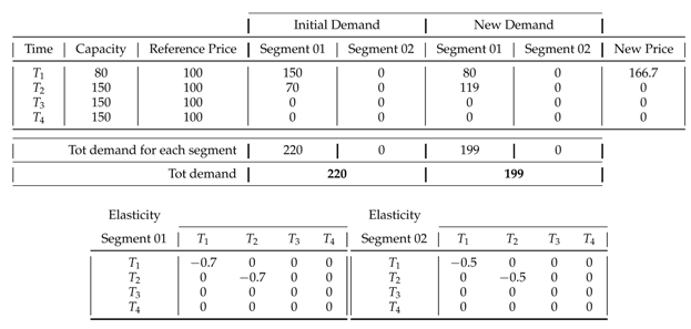 |
In the results, the price is higher in , causing a lower demand in , while the price drops to zero in , causing a higher demand in .
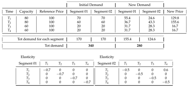
Table 3 shows the change in a case study in which the total load in time-steps and is split among Segments 1 and 2. Self-elasticity values of Segment 1 are higher than those of Segment 2. In order to cut the same total load in time-step , it is necessary to send a higher price signal, because part of the total load now belongs to Segment 2, with lower elasticity. This higher price signal sent in affects the reaction of Segment number 1, that will respond with a higher percentage of demand reduction compared to the basic sub-case (48/100 as compared to 80/150). Hence, the total initial demand for the two sub-cases is the same (220), but the fact that the demand is spread differently among segments with different elasticity, affects the way it is cut in and the way it increases in . In the second sub-case, the presence of a segment with lower elasticity, interestingly causes a lower total new demand compared to the basic sub-case.
Table 3.
Case Study 6.01—second sub-case, data, and results.
Table 3.
Case Study 6.01—second sub-case, data, and results.
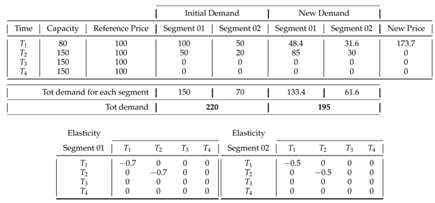 |
Table 4 shows a sub-case in which the two segments have the same demand, but segment number 1 has all loads concentrated in time-step , while segment number 2 has the same amount of loads concentrated in time-step . The amount of loads to be cut is the same for the two segments, but the price signal sent in time-step is lower compared to the price signal sent in time-step , because segment number 1 has higher elasticity values, therefore lower price signals are required to cut the same amount of load. Similarly, the load increase in time-step is higher than the one in because segment number 1 has higher elasticity compared to segment number 2; hence, even though the price reduction in time-steps and is the same, Segment 1 reacts with a higher load increase compared to Segment 2.
Table 4.
Case Study 6.01—third sub-case, data, and results.
Table 4.
Case Study 6.01—third sub-case, data, and results.
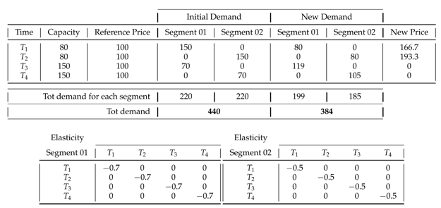 |
Table 5 shows a sub-case in which the load in all time-steps is split among the two segments in and with and . Compared to the third sub-case, the price signal in is higher to cut the same total load, because of the lower elasticity of Segment 2 that now has a load in time-step as well. On the other hand, compared to the third sub-case, the price signal in time-step is lower to cut the same amount of exceeding load, because of the higher elasticity of Cluster 1 that now has a load in time-step .
Table 5.
Case Study 6.01—fourth sub-case, data, and results.
Table 5.
Case Study 6.01—fourth sub-case, data, and results.
 |
6.2. Case Study 6.02
In this second case study, we analyse how the cross-elasticities affect the price signals and how the consequent reactions of the segments affect each other.
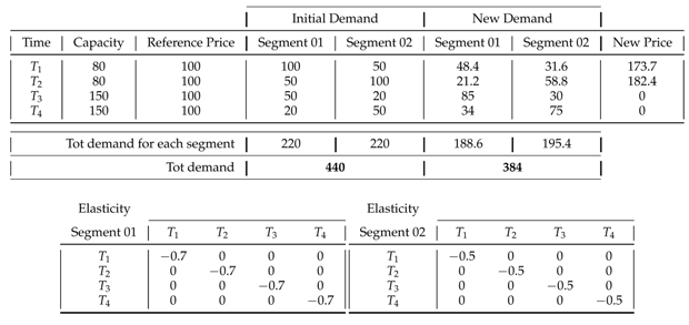
Table 6 represents the basic sub-case in which two segments with the same type of load are placed in time-steps , , and . Results when only self-elasticities are involved are shown. Loads are cut in and and increased in and according to the self-elasticity values of the two segments. As Segment 1 has higher elasticity values, it reacts with higher demand cuts and higher demand reductions compared to Segment 2.
Table 6.
Case Study 6.02—basic sub-case, data, and results.
Table 6.
Case Study 6.02—basic sub-case, data, and results.
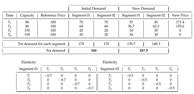 |
Table 7 shows the results when cross-elasticity (below the diagonal of the elasticity matrix) is added for Segment 2. Compared to the basic sub-case, the price signals remain the same, but the load increase in time-step for Segment 2 is higher due to the effect of the cross-elasticity. Hence, even though the price is the same, we note a greater load increase in , and the total new demand in this sub-case is higher than the total new demand of the basic sub-case.
Table 7.
Case Study 6.02—second sub-case, data, and results.
Table 7.
Case Study 6.02—second sub-case, data, and results.
 |
Table 8 shows the results when cross-elasticity (above the diagonal of the elasticity matrix) is added for Segment 2. Compared to the basic sub-case, the price signal in becomes lower, but the total amount of load cut in time remains the same. Due to the cross-elasticity , a lower price signal is required to cut the same amount of total load. However, the way through which the total load is cut is different for the two segments. In particular, due to the price decrease in and due to the cross-elasticity for Segment 2, the new demand in for Segment 2 is lower compared to the second sub-case (hence, a higher demand cut is forecast for Segment 2). Then, to compensate the higher load cut of Segment 2 and keep the total demand equal to the total available capacity, the new demand of Segment 1 in is higher compared to the second sub-case. At the same time, the effect of the cross-elasticity (below the diagonal of the elasticity matrix) for Segment 2 becomes weaker due to the lower price signal sent in . Hence, the demand increase in for Segment 2, compared to the second sub-case, is lower. However, it is important to note that the demand increase of Segment 2 in is still higher than the basic sub-case in which no cross-elasticity was available.
Table 8.
Case Study 6.02—third sub-case, data, and results.
Table 8.
Case Study 6.02—third sub-case, data, and results.
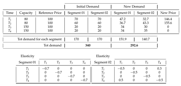 |
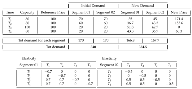
Table 9 shows the results when a lower capacity is assumed in time-steps and additional cross-elasticity values are included below the diagonal of the elasticity matrix. Compared to the basic sub-case, adding a cross-elasticity , for instance, means that we should expect a higher amount of load shifted in time-steps for Segment 2. However, the lower capacity available makes it not possible to allow the demand increase that would be theoretically allowed with that combination of elasticity values. Therefore, compared to the previous sub-cases, the system has to put a higher price in time-step , in order to keep the load increase below the capacity limit. Hence, the price in time-step still drops to motivate the load increase, but it cannot drop to zero in order not to end up with an increase which is too high that would go beyond the available capacity. To compensate that, the price signal in drops to zero, in order to motivate a higher amount of load increase in where enough capacity is available.
Table 9.
Case Study 6.02—fourth sub-case, data, and results.
Table 9.
Case Study 6.02—fourth sub-case, data, and results.
 |
6.3. Case Study 6.03
This third case study has been made to analyse the effects in a sub-case with a very tight capacity limit also in non-critical time-steps. In the previous case studies, there was always enough available capacity in non-critical time-steps to increase the load. In this case study, we impose a very low limit of capacity to investigate the ability of the system to handle the demand cut and increase through pricing.
Table 10 represents the basic sub-case in which two segments with different loads are placed in time-steps , , and . Results when only self elasticities are involved are shown.
Table 10.
Case Study 6.03—basic sub-case, data, and results.
Table 10.
Case Study 6.03—basic sub-case, data, and results.
 |
Table 11 shows the result when the cross-elasticity (above the diagonal of the elasticity matrix) is added for Segment 2. Compared to the basic sub-case, the price signal in time-step is lower, but the demand cut in time-step for Segment 2 is higher (the new demand in time-step for Segment 2 is lower than the basic sub-case, meaning that a higher cut has been done). At the same time, a lower price signal in means a lower cut for Segment 1. Finally, the price in is higher than the basic sub-case, because the capacity is saturated, and therefore it is not possible to allow an increase of load equal to the one that would occur if the price dropped to zero.
Table 11.
Case Study 6.03—second sub-case, data, and results.
Table 11.
Case Study 6.03—second sub-case, data, and results.
 |
7. Limitations and Future Work
The main limitations of the proposed work lie in the uncertainty of the dataset, and in the lack of proper data to build the elasticity matrix. Another limitation lies in the main assumption that all drivers charge their EVs only at a certain period of the day and that they will be sensitive only to the price of electricity, without including the effects of other peak-shaving options. Therefore, future research directions have been identified as follows:
- Further develop the model towards stochastic formulation to consider uncertainty in the input dataset that can affect the quality of the real-time decisions as output.
- Implement a prescriptive analytics approach where machine-learning tools are utilized to predict the elasticity matrix, and the optimization tools are utilized to optimize over the predictions.
- Implement and compare machine-learning approaches and statistical methods for a better definition of the elasticity matrix.
- Include other options for peak-shaving and see how a combination of vehicle to grid and vehicle-to-vehicle options together would affect the decision-making process of indirect control through elasticities.
8. Conclusions
This paper presented a method based on price elasticities to produce price signals for indirect control and capacity scheduling for electric vehicle charging.
The study demonstrates that understanding drivers’ elasticity is essential and crucial to build pricing models and properly handle capacity shortages in charging stations and the grid. Both self elasticities, within a time-period, and cross-elasticities between time-periods plays a role. The paper illustrates the effects in a number of case studies and sensitivity analyses. In addition, suggestions for how to model price discrimination are provided.
More research should be done in this field in order to provide the data needed for this type of scheduling, in particular empirical studies to identify the needed elasticity matrices for different consumer clusters in different times of the day and different areas. This research area is currently completely uncovered, but our results show that once elasticity data for drivers exist, they provide the basis for effective peak pricing of electric vehicle charging.
Further model extensions can be built to handle the uncertainty in the elasticity definition. Moreover, indirect control models should be integrated with models for the optimal design and expansion of charging sites.
Author Contributions
Conceptualization, A.T. and C.B.; methodology, A.T. and C.B.; software, C.B.; validation, C.B.; formal analysis, C.B.; investigation, C.B.; resources, C.B.; data curation, C.B.; writing—original draft preparation, C.B. and A.T.; writing—review and editing, C.B. and A.T.; visualization, C.B.; supervision, A.T.; project administration, A.T.; funding acquisition, A.T. All authors have read and agreed to the published version of the manuscript.
Funding
This research was funded by the Chargeflex project NRC grant 239755.
Institutional Review Board Statement
Not applicable.
Informed Consent Statement
Not applicable.
Conflicts of Interest
The authors declare no conflict of interest.
References
- Anenberg, S.; Miller, J.; Henze, D.; Minjares, R. A Global Snapshot of the Air Pollution-Related Health Impacts of Transportation Sector Emissions in 2010 and 2015; International Council on Clean Transportation: Washington, DC, USA, 2019. [Google Scholar]
- Kontovas, C.A.; Psaraftis, H.N. Transportation Emissions: Some Basics. In Green Transportation Logistics; Springer: Berlin/Heidelberg, Germany, 2016; pp. 41–79. [Google Scholar]
- Bordin, C.; Tomasgard, A. SMACS MODEL, a stochastic multihorizon approach for charging sites management, operations, design, and expansion under limited capacity conditions. J. Energy Storage 2019, 26, 100824. [Google Scholar] [CrossRef]
- Ager-Hanssen, S.B.; Myhre, S.O. Utilization of the Flexibility Potential of Electric Vehicles-an Alternative to Distribution Grid Reinforcements. Master’s Thesis, NTNU, Trondheim, Norway, 2015. [Google Scholar]
- Heussen, K.; You, S.; Biegel, B.; Hansen, L.H.; Andersen, K.B. Indirect control for demand-side management-A conceptual introduction. In Proceedings of the 2012 3rd IEEE PES Innovative Smart Grid Technologies Europe (ISGT Europe), Berlin, Germany, 14–17 October 2012; pp. 1–8. [Google Scholar]
- Liu, K.; Zou, C.; Li, K.; Wik, T. Charging pattern optimization for lithium-ion batteries with an electrothermal-aging model. IEEE Trans. Ind. Inform. 2018, 14, 5463–5474. [Google Scholar] [CrossRef]
- Liu, K.; Hu, X.; Yang, Z.; Xie, Y.; Feng, S. Lithium-ion battery charging management considering economic costs of electrical energy loss and battery degradation. Energy Convers. Manag. 2019, 195, 167–179. [Google Scholar] [CrossRef]
- Liu, K.; Li, K.; Ma, H.; Zhang, J.; Peng, Q. Multi-objective optimization of charging patterns for lithium-ion battery management. Energy Convers. Manag. 2018, 159, 151–162. [Google Scholar] [CrossRef]
- Bordin, C. Mathematical Optimization Applied to Thermal and Electrical Energy Systems. Ph.D. Thesis, Alma Mater Studiorum Università di Bologna, Bologna, Italy, 2015. [Google Scholar]
- Shuai, W.; Maillé, P.; Pelov, A. Charging electric vehicles in the smart city: A survey of economy-driven approaches. IEEE Trans. Intell. Transp. Syst. 2016, 17, 2089–2106. [Google Scholar] [CrossRef] [Green Version]
- Nour, M.; Said, S.M.; Ali, A.; Farkas, C. Smart charging of electric vehicles according to electricity price. In Proceedings of the 2019 International Conference on Innovative Trends in Computer Engineering (ITCE), Aswan, Egypt, 2–4 February 2019; pp. 432–437. [Google Scholar]
- Seddig, K.; Jochem, P.; Fichtner, W. Two-stage stochastic optimization for cost-minimal charging of electric vehicles at public charging stations with photovoltaics. Appl. Energy 2019, 242, 769–781. [Google Scholar] [CrossRef]
- Skolthanarat, S.; Somsiri, P.; Tungpimolrut, K. Contribution of Real-Time Pricing to Impacts of Electric Cars on Distribution Network. In Proceedings of the 2019 IEEE Industry Applications Society Annual Meeting, Baltimore, MD, USA, 29 September–3 October 2019; pp. 1–5. [Google Scholar]
- Yu, R.; Yang, W.; Rahardja, S. A statistical demand-price model with its application in optimal real-time price. IEEE Trans. Smart Grid 2012, 3, 1734–1742. [Google Scholar] [CrossRef]
- Yu, R.; Yang, W.; Rahardja, S. Optimal real-time price based on a statistical demand elasticity model of electricity. In Proceedings of the 2011 IEEE First International Workshop on Smart Grid Modeling and Simulation (SGMS), Brussels, Belgium, 17 October 2011; pp. 90–95. [Google Scholar]
- Sadeghian, O.; Nazari-Heris, M.; Abapour, M.; Taheri, S.S.; Zare, K. Improving reliability of distribution networks using plug-in electric vehicles and demand response. J. Mod. Power Syst. Clean Energy 2019, 7, 1189–1199. [Google Scholar] [CrossRef] [Green Version]
- de Sá Ferreira, R.; Barroso, L.A.; Lino, P.R.; Carvalho, M.M.; Valenzuela, P. Time-of-use tariff design under uncertainty in price-elasticities of electricity demand: A stochastic optimization approach. IEEE Trans. Smart Grid 2013, 4, 2285–2295. [Google Scholar] [CrossRef]
- Hu, J.; Si, C.; Lind, M.; Yu, R. Preventing distribution grid congestion by integrating indirect control in a hierarchical electric vehicles’ management system. IEEE Trans. Transp. Electrif. 2016, 2, 290–299. [Google Scholar] [CrossRef] [Green Version]
- Lijesen, M.G. The real-time price elasticity of electricity. Energy Econ. 2007, 29, 249–258. [Google Scholar] [CrossRef]
- Kirschen, D.S.; Strbac, G.; Cumperayot, P.; de Paiva Mendes, D. Factoring the elasticity of demand in electricity prices. IEEE Trans. Power Syst. 2000, 15, 612–617. [Google Scholar] [CrossRef] [Green Version]
- Cartenì, A.; Cascetta, E.; de Luca, S. A random utility model for park & carsharing services and the pure preference for electric vehicles. Transp. Policy 2016, 48, 49–59. [Google Scholar]
- Paterakis, N.G.; Taşcıkaraoğlu, A.; Erdinc, O.; Bakirtzis, A.G.; Catalao, J.P. Assessment of demand-response-driven load pattern elasticity using a combined approach for smart households. IEEE Trans. Ind. Inform. 2016, 12, 1529–1539. [Google Scholar] [CrossRef]
- Aalami, H.; Moghaddam, M.P.; Yousefi, G. Demand response modeling considering interruptible/curtailable loads and capacity market programs. Appl. Energy 2010, 87, 243–250. [Google Scholar] [CrossRef]
- Venkatesan, N.; Solanki, J.; Solanki, S.K. Residential Demand Response model and impact on voltage profile and losses of an electric distribution network. Appl. Energy 2012, 96, 84–91. [Google Scholar] [CrossRef]
- Ghasemi, A.; Mortazavi, S.S.; Mashhour, E. Hourly demand response and battery energy storage for imbalance reduction of smart distribution company embedded with electric vehicles and wind farms. Renew. Energy 2016, 85, 124–136. [Google Scholar] [CrossRef]
- Rathore, C.; Roy, R. Impact of wind uncertainty, plug-in-electric vehicles and demand response program on transmission network expansion planning. Int. J. Electr. Power Energy Syst. 2016, 75, 59–73. [Google Scholar] [CrossRef]
- Behboodi, S.; Chassin, D.P.; Crawford, C.; Djilali, N. Renewable resources portfolio optimization in the presence of demand response. Appl. Energy 2016, 162, 139–148. [Google Scholar] [CrossRef] [Green Version]
- Geng, L.; Lu, Z.; He, L.; Zhang, J.; Li, X.; Guo, X. Smart charging management system for electric vehicles in coupled transportation and power distribution systems. Energy 2019, 189, 116275. [Google Scholar] [CrossRef]
- Kannan, A.; Tumuluru, V.K. Behavioral Modeling of Electric Vehicles Using Price Elasticities. In Proceedings of the 2018 IEEE Innovative Smart Grid Technologies-Asia (ISGT Asia), Singapore, 22–25 May 2018; pp. 593–598. [Google Scholar]
- Srivatsa, C.R.; Rengarajan, D.; Tumuluru, V.K. Modeling demand flexibility of electric vehicles. In Proceedings of the 2017 IEEE International Conference on Smart Grid Communications (SmartGridComm), Dresden, Germany, 23–27 October 2017; pp. 363–368. [Google Scholar]
- Tang, W.; Yang, H.T. Optimal operation and bidding strategy of a virtual power plant integrated with energy storage systems and elasticity demand response. IEEE Access 2019, 7, 79798–79809. [Google Scholar] [CrossRef]
- Mohiti, M.; Monsef, H.; Anvari-Moghaddam, A.; Guerrero, J.; Lesani, H. A decentralized robust model for optimal operation of distribution companies with private microgrids. Int. J. Electr. Power Energy Syst. 2019, 106, 105–123. [Google Scholar] [CrossRef]
- Jiang, J.; Kou, Y.; Bie, Z.; Li, G. Optimal real-time pricing of electricity based on demand response. Energy Procedia 2019, 159, 304–308. [Google Scholar] [CrossRef]

Publisher’s Note: MDPI stays neutral with regard to jurisdictional claims in published maps and institutional affiliations. |
© 2021 by the authors. Licensee MDPI, Basel, Switzerland. This article is an open access article distributed under the terms and conditions of the Creative Commons Attribution (CC BY) license (https://creativecommons.org/licenses/by/4.0/).