Flow Pattern and Resistance Characteristics of Gas–Liquid Two-Phase Flow with Foam under Low Gas–Liquid Flow Rate

Abstract

To reduce the cost of arranging air foam flooding equipment at each wellhead, a method of establishing centralized air foam flooding injection stations is proposed. The flow pattern and resistance characteristics of air foam flooding mixtures in different initial conditions are studied. Experimental results indicate that the probability density function of stratified flow is obtained by comparing stainless steel and transparent pipes. If the gas–liquid ratio is kept constant, then the shape of the probability density function remains unchanged in both stainless steel and transparent tubes. Meanwhile, the flow pattern under the gas–liquid ratio is determined by comparing the image recognition results with the probability density function, and a formula for calculating the resistance and pressure drop of the gas and liquid two-phase flow in the horizontal and upward pipes is established. Compared with the experiments, the error results of the calculation are small. Thus, the proposed equations can be used to predict the flow resistance of real air foam flooding.

1. Introduction

Oil is a very important energy source, so countries all over the world have always attached great importance to the development and utilization of oil. Petroleum is mainly used as fuel oil and gasoline as well as a raw material for many chemical industrial products, such as solutions, fertilizers, pesticides, and plastics. At present, China’s oil consumption accounts for approximately 19% of China’s total energy consumption, but China’s current dependence on foreign oil exceeds 70%. Ensuring the safe supply of oil is not only related to national life but also affects national security and stability. Oil is the cornerstone of national strategies, the basis of realizing military strategies, and the strong driving force of economic development [1]. In recent years, the proven reserves of low and ultra-low permeability reservoirs have accounted for a large proportion of the total reserves in China, and the research on the enhanced oil recovery (EOR) of such reservoirs is becoming increasingly important. Meanwhile, low and ultra-low permeability reservoirs have been mainly developed by water injection [2]. Many oilfields have entered the middle and high water cut stages too early, and the balance of injection and production is difficult to maintain due to the high water injection pressure in the later stage. In addition, the cost of water injection technology is high and the economic benefit is low. Therefore, economical and effective recovery methods for low and ultra-low permeability reservoirs are the new research topic. Given that oil wells are distributed in a region, equipping each oil well with a set of production equipment will increase the cost of production. Using a set of production equipment and performing the injection into each oil well through a pipeline will greatly reduce the cost of oil production. Air foam flooding technology is a kind of oil displacement technology that uses foam as the displacement medium. The technology integrates the two technical advantages of air drive and surfactant flooding. The technology is relatively simple, and the effect of EOR is obvious. Air foam flooding has become an important replacement technology for water flooding and polymer flooding in recent years [3].

As one of the three oil recovery technologies in the world, foam flooding has gradually become a widely used EOR method in the oil and gas fields. The main mechanism of EOR by foam flooding is to increase the sweep volume and improve the efficiency of oil washing. Meanwhile, the surfactant in foam liquid can reduce the interfacial tension and adjust the oil–water mobility ratio. Foam fluid has been widely used in the development direction of oil and gas because of its unique properties, which can be traced back to the 1950s. Fried et al. [4] were the first scholars to study foam flooding in the 1950s. They believed that foam reduces the relative permeability of the gas phase in the rock void and delays the breakthrough of gas, thereby enhancing the recovery efficiency. It is also found that the greater the foam strength, the stronger the ability to prevent air breakthrough [5]. Jensen et al. [6] found that the oil saturation in porous media affects the stability of foam. When the oil saturation exceeds a certain range, the foam becomes unstable or even fails to form. Many researchers have shown that adding polymer to the foam system can increase the foam thickness, reduce the adsorption of surfactant on rocks, enhance the stability of foam, and greatly improve the displacement efficiency [7,8]. With the rise of nanomaterials, researchers have mixed nanoparticles into foam systems to achieve foam stability and improve performance. The results show that nanoparticles and surfactants play a synergistic role in stabilizing foam. The addition of nanoparticles has great potential in the selective plugging of high permeability regions in heterogeneous reservoirs [9,10,11,12].

At present, the research on air foam flooding is mainly focused on micro fracture plugging in low permeability reservoirs. It is mainly used to expand the swept volume of the follow-up injection fluid, reduce the water yield and improve the oil recovery. Few studies have been conducted on the surface transportation of the injection liquid, and most of them focus on the flow pattern and resistance of air and water in the surface transportation process. Many kinds of detection and information processing technologies for flow pattern recognition currently exist, and they are all in development. In recent years, on the basis of the analysis of and experiments on flow mechanism, many flow pattern diagrams have been proposed to help in flow pattern identification, and the Baker and Mandhane [13] flow pattern diagrams are the most representative. Ewing et al. [14] used camera technology to record the change in gas–water two-phase flow pattern in a horizontal pipe and compared it with the flow pattern diagram proposed by Baker. Kang et al. [15,16] proposed two general flow pattern diagrams for horizontal and vertical risers using broad data. In addition to the flow pattern map, the high-speed camera can also be used for flow pattern recognition. Rafalko et al. [17] proposed a two-phase flow pattern recognition method with fast recording and simple, unfiltered image analysis. Amaral et al. [18] proposed a new technology for automatically estimating bubble parameters (such as frequency, size, and velocity) through the video analysis of a high-speed camera to measure bubbles in horizontal pipes. The contour and velocity of bubbles in observation images are detected and estimated by image processing technology. The findings indicate that the calculated parameters are consistent with the theoretical prediction. Hernández et al. [19] carried out an experimental study on the gas–water two-phase flow in a circular pipe with an outer diameter of 155 mm, an inner diameter of 60 mm, and a length of 10.5 m. The average velocity of bubbles is estimated using high-speed video technology and particle image velocimetry combined with Annular Wire-Mesh Sensor (AWMS). A new technology for measuring bubble channel frequency, bubble length and slug length based on AWMS is proposed. Wang et al. [20] conducted an experimental study on the pressure oscillation caused by lateral steam injection in a horizontal tube. According to the probability density function (PDF), the effects of the steam mass flow rate, the supercooled water flow rate, and temperature on the distribution amplitude of pressure oscillation were analyzed. Rodrigues et al. [21] used resistance sensors to collect data from the horizontal air–water slug flow and correlated the influence of the apparent velocity of liquid and gas with the probability density function (PDF) of parameter changes observed in the development of plug flow along the pipe section. Orkriszewski et al. [22] summarized the calculation methods of multiple pressure gradients, analyzed and verified the production data of 148 oil wells, and proposed pressure drop calculation methods for bubble, slug, transition, and annular mist flows. Beggs and Brill [23] used water and air as the flow medium and two translucent polypropylene pipes as the measuring pipe section. Through numerous experiments, a pressure drop calculation method suitable for horizontal wells and undulating pipelines was obtained. Imamura et al. [24] studied the influence of pipe diameter on pressure drop and used a large-diameter vertical pipe for pressure drop simulation. The findings indicate that the larger the friction coefficient is, the larger the pressure drop related to the pipe diameter is. Kosuke et al. [25] measured the pressure drop in the horizontal U-bend through an experiment, compared the result with that using the Chisholm method, and found that the measured value was near the experimental value. Bhagwat et al. [26] established a gas–liquid two-phase drift flow model. This model is not based on the judgment of flow pattern when calculating liquid holdup. Substantial experimental data show that this model has a high calculation accuracy.

Most of the current studies on air foam flooding mainly focus on the plugging ability of the air and foam injected into the ground, the stability of foam, and the enhancement of oil recovery. Most of the existing research on the surface transportation process focuses on the transportation of water and air. Moreover, the research focuses on the identification and calculation of flow patterns in horizontal and inclined pipes and the theoretical calculation of resistance. Few studies have been conducted on the flow patterns and resistance of long-distance air and foam mixtures for surface pipelines. Therefore, this paper focuses on the flow patterns and resistance characteristics of horizontal and inclined pipes in air foam flooding. In this study, the high-speed camera and PDF methods are used to study the flow pattern under different gas–liquid ratios, and the differential pressure method is used to study the resistance characteristics under different gas–liquid ratios.

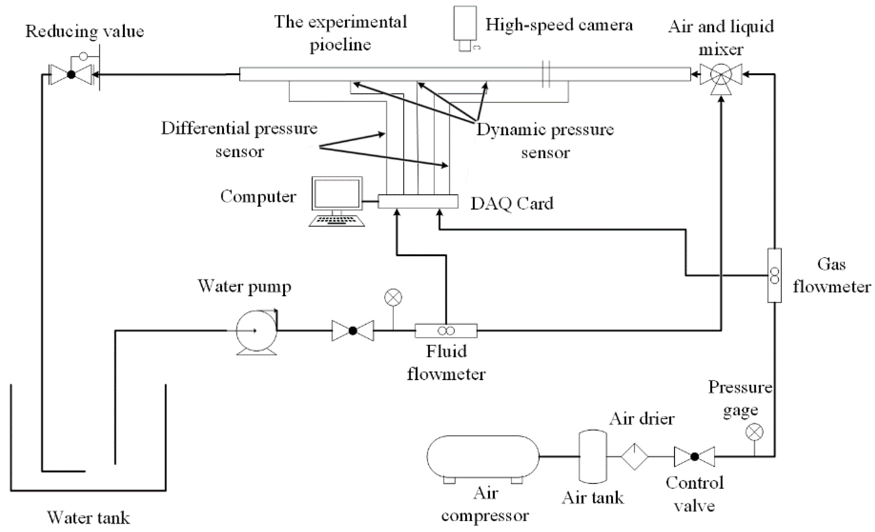
2. Experimental System

We carried out indoor experiments on the changing laws of flow patterns under different initial conditions and the characteristics of resistance changes under different flow patterns. Combining the calculation theory of gas–liquid two-phase resistance and the research on gas–liquid two-phase flow theory, the key technology of gas–liquid two-phase mixing with foam-assisted oxygen-reducing air purging is proposed under different conditions.

The experimental device is shown in Figure 1. The fluid used in the experiment is a mixture of foaming agent and foam stabilizer, and air was added to water. The experimental section is horizontal, inclined upward at 10°, inclined upward at 20°, inclined downward at 10°, and inclined downward at 20°. The experimental tube is 3 m long. To facilitate the observation of the flow pattern in the pipeline, the experimental tube section is a transparent tube. Meanwhile, to measure the resistance under high pipeline pressure, the experimental pipe section is a stainless steel pipe.

In this experiment, three dynamic pressure sensor measuring points, as shown in Figure 1, and two differential pressure sensor measuring points, as shown in Figure 1, are installed. The distance between the measuring points is 500 mm, and the pipe’s inner diameter is 50 mm. The instantaneous pressure collection in the experimental pipeline is completed by the three dynamic pressure sensors, and the measurement accuracy error is ±0.2 kPa. The differential pressure sensor is used for differential pressure collection, and the measurement accuracy is ±0.25%.

During the experiment, the throttle valve at the liquid inlet is first adjusted to maintain the liquid flow rate at a certain value. Then, the gas flow is gradually increased to reach the required experimental parameters, and the corresponding gas–liquid flow, flow pattern, and pressure parameters for different working conditions are recorded. The pressure in the pipeline is changed by adjusting the back pressure valve. In the experiment, the converted flow velocity range of the gas phase is 0.212–0.637 m/s, and the converted flow velocity range of the liquid phase is 0.071–0.141 m/s.

3. Data Processing Method

A high-speed camera is used in visualizing the pipeline experiment. Meanwhile, the dynamic pressure sensor is used to record the pressure fluctuation signal. The pictures taken by the high-speed camera are processed by MATLAB. The gas and liquid phases are distinguished to facilitate the judging of the flow pattern. Meanwhile, the pressure signal obtained by the dynamic pressure sensor is processed by the PDF, the corresponding characteristic graph is obtained, and the flow pattern is judged according to the unique characteristic graph.

(1) Image Processing.

The high-speed camera method uses a high-speed camera to acquire two-phase flow images, uses digital image processing technology for image processing, and builds a classifier for flow pattern recognition. This method has many advantages, such as visualization, non-invasiveness, and good instantaneity. The current research work on flow pattern identification based on the high-speed camera method mostly relies on digital image processing to extract different image features.

(2) Probability density function (PDF).

According to PDF theory, the signal’s minimum and maximum values are divided into several intervals, and the ratio of the number of times the signal amplitude appears in each interval to the total sampling points is used as the probability estimate of this interval. The PDF represents the probability that the instantaneous amplitude falls within the specified range. The function will change if the amplitude of the range is different.

$$P_i=\frac{n_i}{N}$$

(1)

4. Flow Pattern Analysis of Two-Phase Flow

The gas–liquid two-phase flow pattern with foam is studied in this paper. The mixture of air and foam in water is flowing in the transparent and stainless steel pipes with a diameter of 50 mm. The flow in the tube lying horizontally, inclined upward at 10° and inclined upward at 20°, was studied. First, the typical flow patterns in the horizontal and inclined tubes were obtained by visual inspection and high-speed photography. Meanwhile, high-frequency dynamic pressure sensor signal data are obtained, the flow patterns of transparent and stainless steel pipes are compared, and the feasibility and applicability of the PDF method are verified.

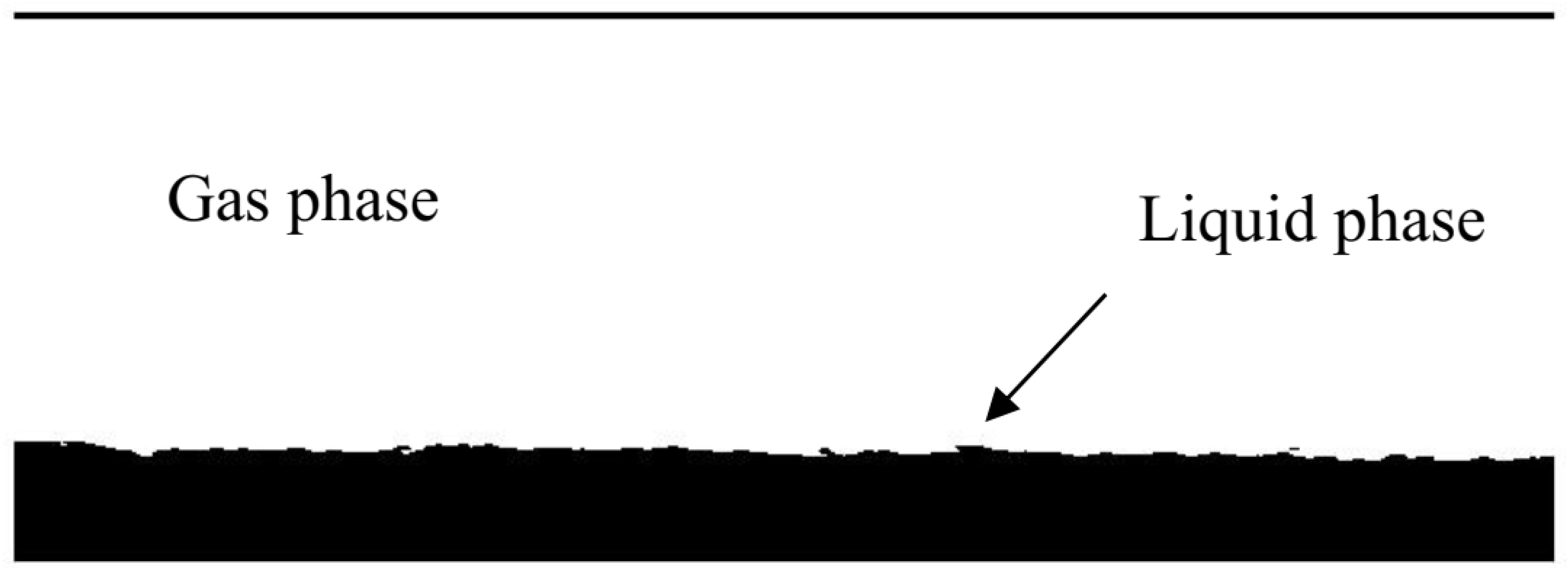
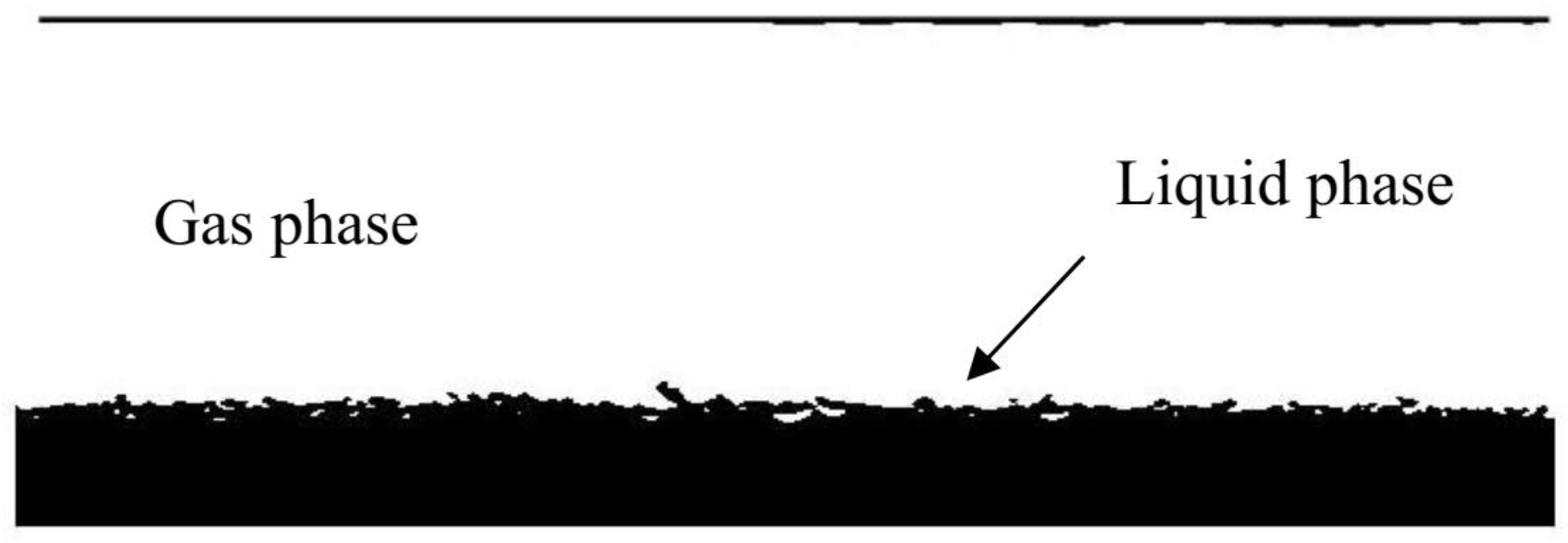
4.1. Flow Pattern of Two-Phase Flow in Horizontal Pipe

When the experimental pipeline is horizontal, the foaming agent and the foam stabilizer are added in proportion to the water. Meanwhile, the back pressure valve is adjusted to increase the pressure in the pipeline. When the pipeline is a transparent pipeline, the pressure in the pipeline is 0.15 and 0.2 MPa. When the experimental section is a stainless steel pipeline, the pressure in the pipeline is 0.2, 0.4, and 0.6 MPa. In the experiment, the flow of liquid is 1 m³/h, and the flow of gas is 1.5–4 m³/h.

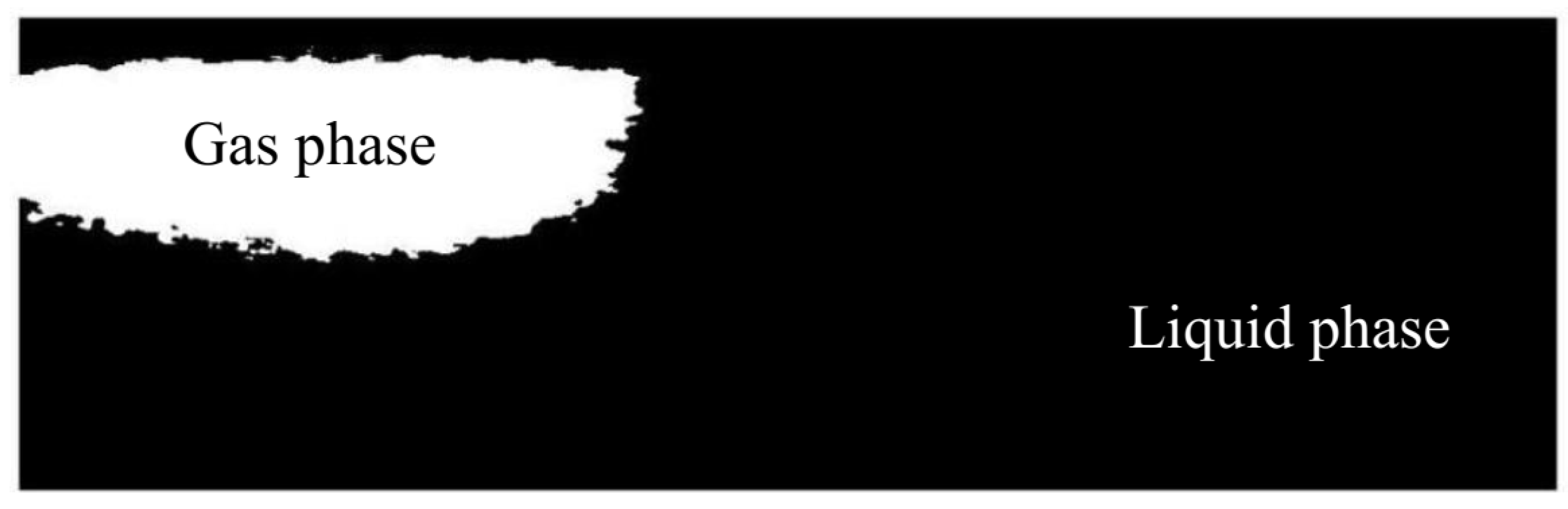
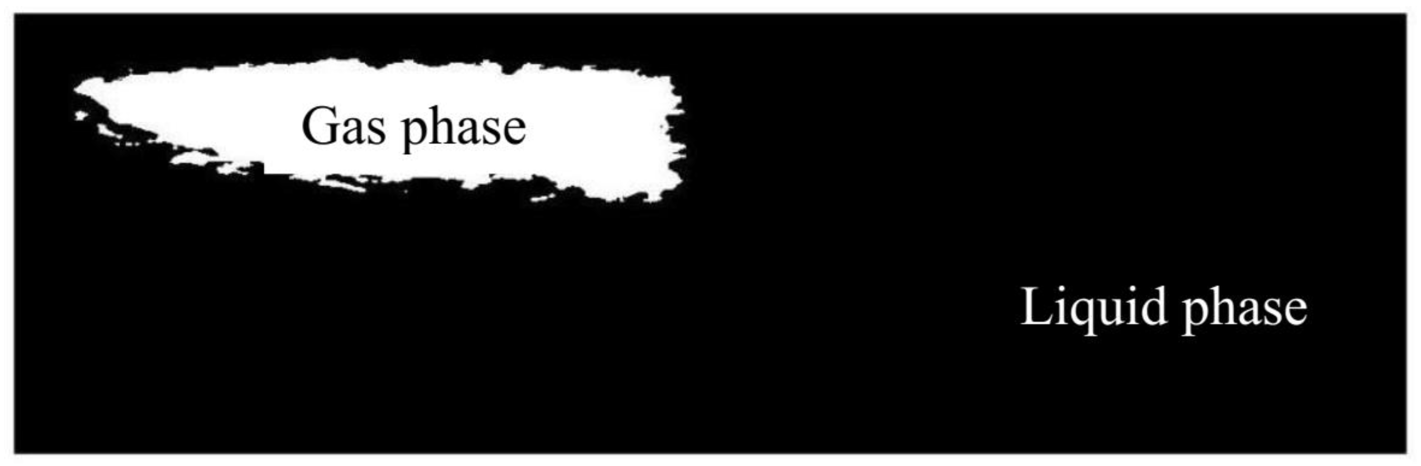
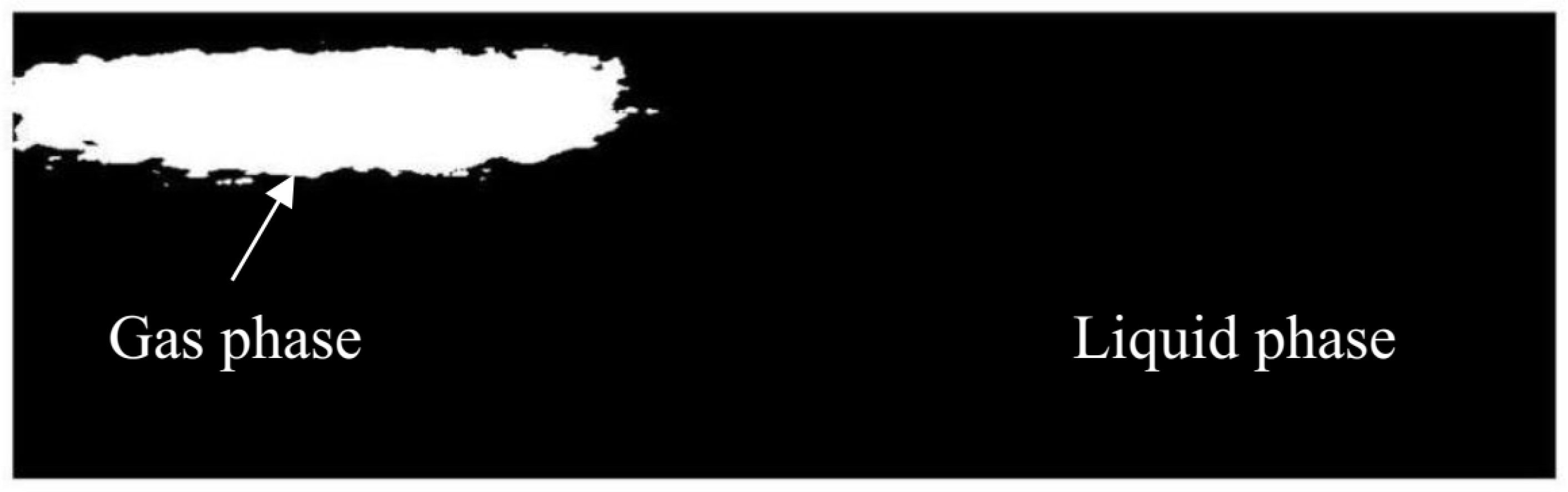
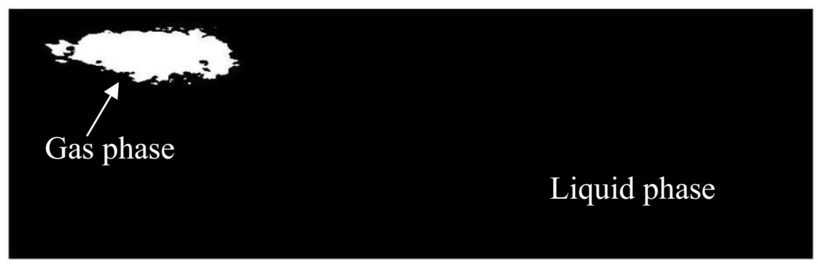
4.1.1. Image Processing

Table 1. Flow patterns of horizontal pipes at different pipe pressures.

Pressure	1.5 m3/h	2 m3/h	2.5 m3/h	3 m3/h	3.5 m3/h	4 m3/h
0.15 MPa	Stratified flow	Stratified flow	Stratified flow	Stratified flow	Stratified flow	Stratified flow
0.2 MPa	Stratified flow	Stratified flow	Stratified flow	Stratified flow	Stratified flow	Stratified flow
0.4 MPa	Stratified flow	Stratified flow	Stratified flow	Stratified flow	Stratified flow	Stratified flow
0.6 MPa	Stratified flow	Stratified flow	Stratified flow	Stratified flow	Stratified flow	Stratified flow

shows the flow pattern of different pipe pressures at the horizontal pipe. When the liquid flow rate is 1 m³/h and the gas flow rate is 1.5–4 m³/h, the flow pattern is stratified flow. Figure 2 presents a picture taken after image processing when the liquid flow rate is 1 m³/h and the gas flow rate is 3 m³/h under 0.15 MPa. Figure 3 presents a picture taken after image processing when the liquid flow rate is 1 m³/h and the gas flow rate is 3 m³/h under 0.2 MPa. Figure 2 and Figure 3 indicate that the liquid is at the bottom of the pipe, the interface between the liquid and the gas is clear, and the flow is stable and stratified flow.

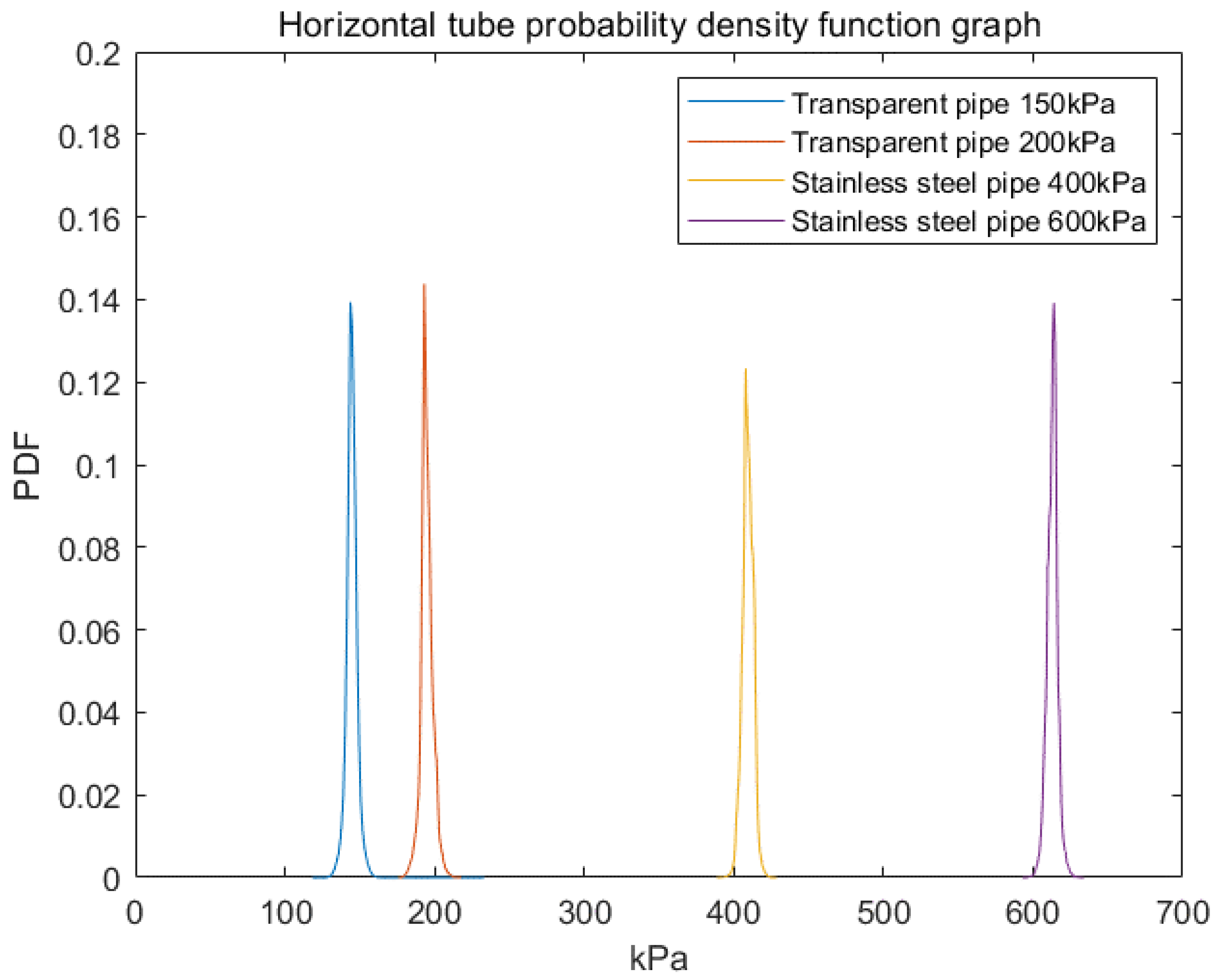
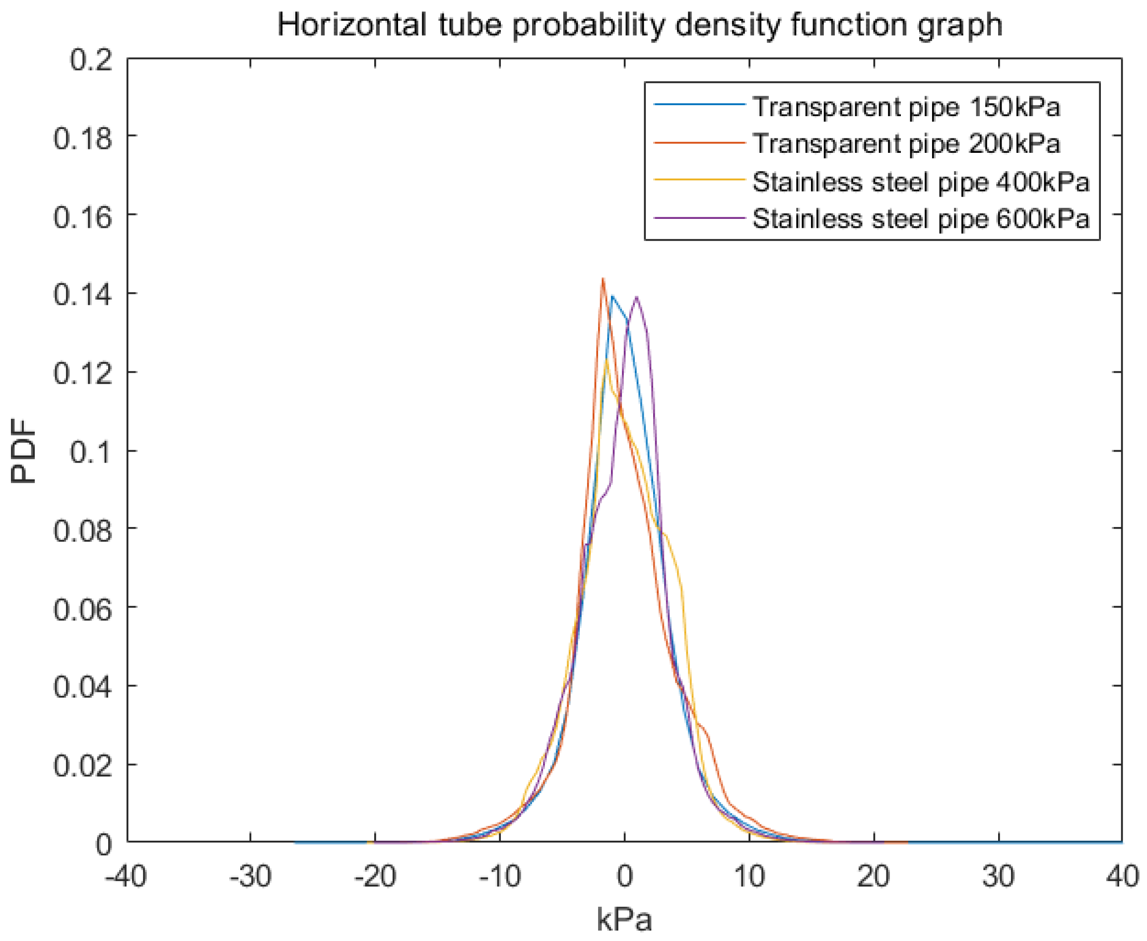
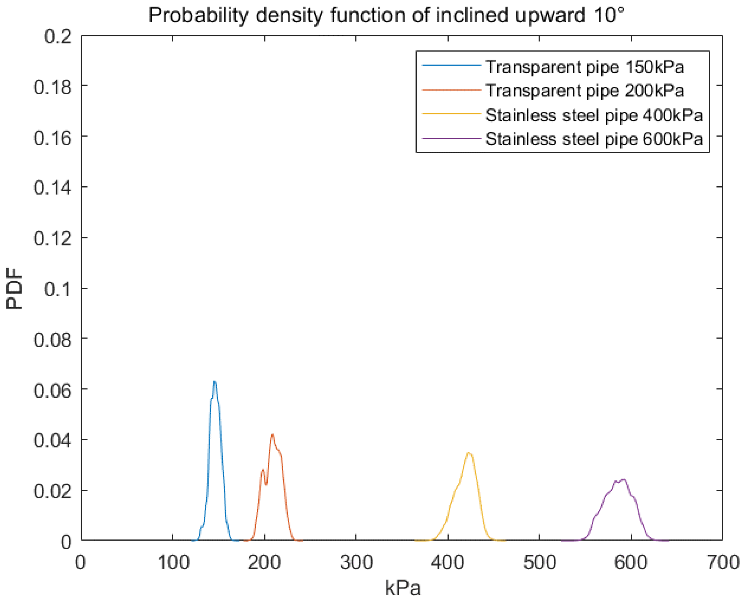
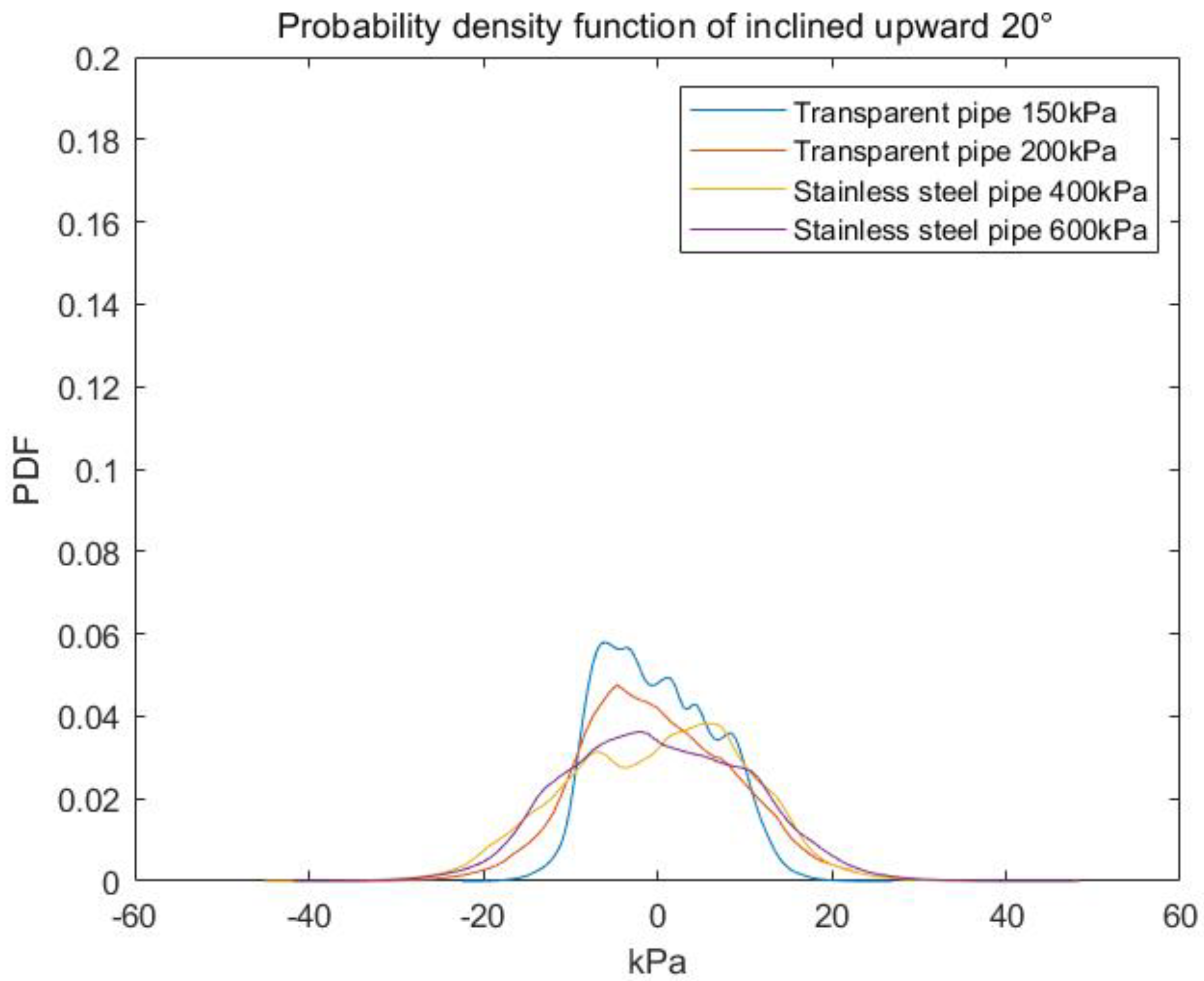
4.1.2. Probability Density Function Graph

When the experimental section is a transparent pipeline, in addition to taking pictures, a high-frequency dynamic pressure sensor is also used to collect pressure signals, which are processed by PDFs to obtain a PDF graph. When the experimental section is a stainless steel pipe, a high-frequency dynamic pressure sensor is also used to collect pressure signals. Then, PDF processing is utilized to obtain a PDF graph, which is compared with that of the transparent tube. In Figure 4, when the pressure is 0.15 and 0.2 MPa, the PDF diagram is obtained by the transparent tube, and when the pressure is 0.4 and 0.6 MPa, the PDF diagram is obtained by the stainless steel pipe. At this time, the liquid flow rate is 1 m³/h and the gas flow rate is 3 m³/h, and the pressure PDF diagram of the stainless steel pipe is similar to that of the transparent pipe. Furthermore, the flow pattern of the stainless steel pipe is laminar. Figure 5 is the probability density diagram after subtracting the pipeline pressure. The diagram shows that the probability density graphs collected under different pressures are similar. Thus, the PDF method can be used to measure the flow pattern.

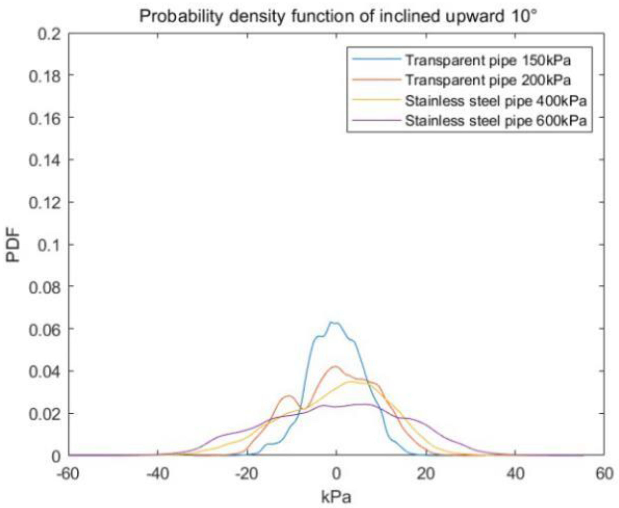
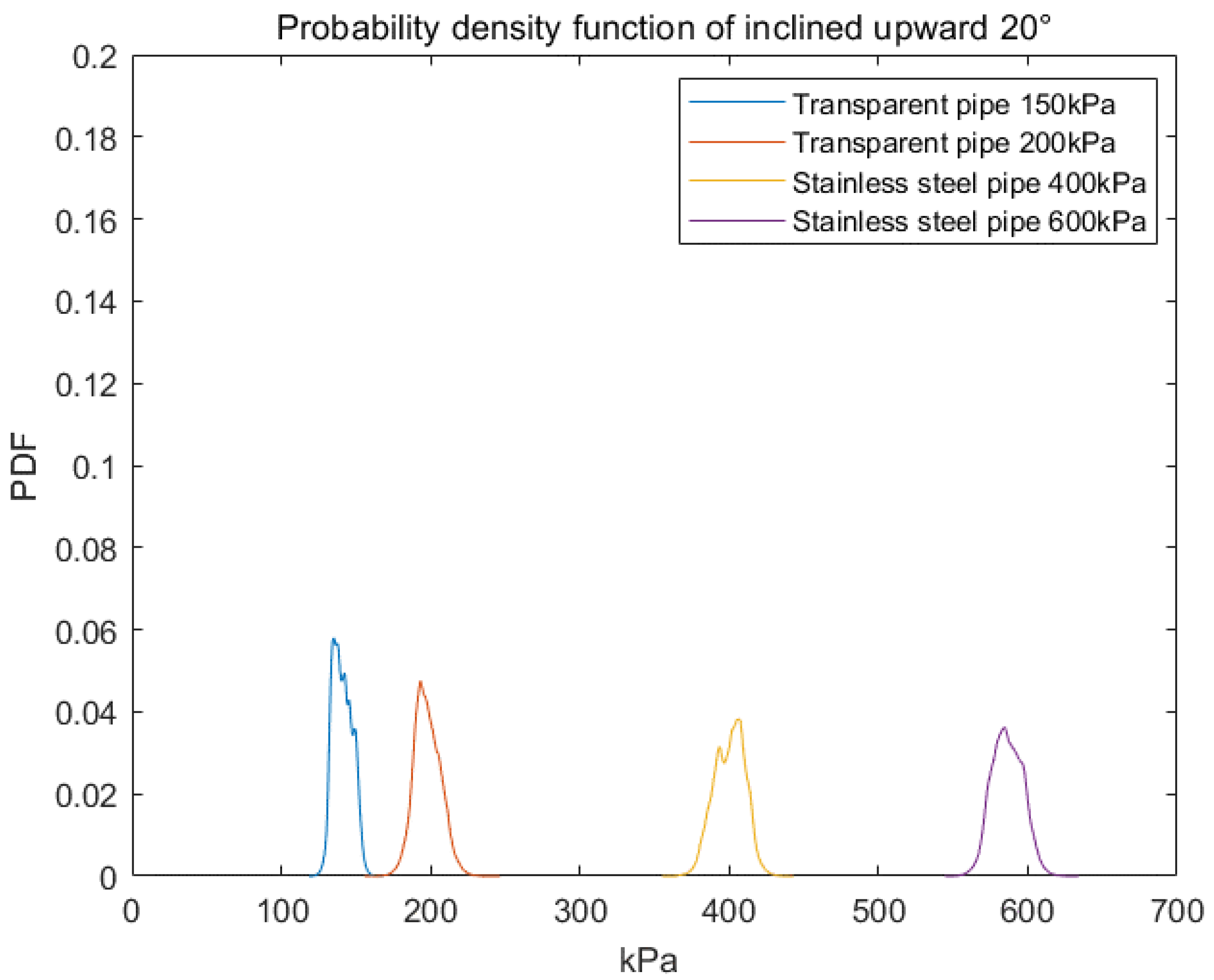
4.2. Two-Phase Flow Pattern in Inclined Upward Pipe

When the experimental pipeline is inclined upward, the experimental conditions are the same as those in the horizontal pipeline. The pressure in the transparent pipe is 0.15 and 0.2 MPa. The pressure in the stainless steel pipeline is 0.2, 0.4, and 0.6 MPa. In the experiment, the liquid flow rate is 1 m³/h, and the gas flow rate is 1.5–4 m³/h. Meanwhile, the inclination angle of the experimental pipe is 10° and 20°.

4.2.1. Tilt Up 10°

(1) Image processing.

As shown in

Table 2. Flow patterns of different pipe pressures inclined up to 10°.

Pressure	1.5 m3/h	2 m3/h	2.5 m3/h	3 m3/h	3.5 m3/h	4 m3/h
0.15 MPa	Slug flow	Slug flow	Slug flow	Slug flow	Slug flow	Slug flow
0.2 MPa	Slug flow	Slug flow	Slug flow	Slug flow	Slug flow	Slug flow
0.4 MPa	Slug flow	Slug flow	Slug flow	Slug flow	Slug flow	Slug flow
0.6 MPa	Slug flow	Slug flow	Slug flow	Slug flow	Slug flow	Slug flow

, the results show the flow pattern with different pipe pressures when the inclination is 10 ° upward. When the liquid flow rate is 1 m³/h and the gas flow rate is 1.5–4 m³/h, the flow pattern is slug flow. Figure 6 presents a picture taken after image processing when the liquid flow rate is 1 m³/h and the gas flow rate is 3 m³/h under 0.15 MPa. Figure 7 is a picture taken after image processing when the liquid flow rate is 1 m³/h and the gas flow rate is 3 m³/h under 0.2 MPa. The figure shows that the white area is where the gas phase is located, and the black area is where the liquid phase and slug are located, so the flow is slug flow.

(2) Probability density function graph.

The PDF graph is obtained in the same way as the horizontal tube. In Figure 8, when the pressure is 0.15 and 0.2 MPa, the PDF diagram is obtained by the transparent tube, and when the pressure is 0.4 and 0.6 MPa, the PDF diagram is obtained by the stainless steel pipe. At this time, the liquid flow rate is 1 m³/h and the gas flow rate is 3 m³/h, and the pressure PDF diagram of the stainless steel pipe is similar to that of the transparent pipe. As shown in Figure 9, it is the probability density diagram after subtracting the pipeline pressure. The diagram shows that the probability density diagrams collected under different pressures are similar, proving that the flow pattern in the stainless steel pipe is also slug flow.

4.2.2. Tilt Up 20°

(1) Image processing.

Table 3. Flow patterns of different pipe pressures inclined up to 20°.

Pressure	1.5 m3/h	2 m3/h	2.5 m3/h	3 m3/h	3.5 m3/h	4 m3/h
0.15 MPa	Slug flow	Slug flow	Slug flow	Slug flow	Slug flow	Slug flow
0.2 MPa	Slug flow	Slug flow	Slug flow	Slug flow	Slug flow	Slug flow
0.4 MPa	Slug flow	Slug flow	Slug flow	Slug flow	Slug flow	Slug flow
0.6 MPa	Slug flow	Slug flow	Slug flow	Slug flow	Slug flow	Slug flow

shows the flow pattern with different pipe pressures when the inclination is 20° upward. When the liquid flow rate is 1 m³/h and the gas flow rate is 1.5–4 m³/h, the flow pattern is slug flow. Figure 10 is a picture taken after image processing when the liquid flow rate is 1 m³/h and the gas flow rate is 3 m³/h under 0.15 MPa. Figure 11 is a picture after image processing when the liquid flow rate is 1 m³/h and the gas flow rate is 3 m³/h under 0.2 MPa. The figure shows that the white area is where the gas phase is located, and the black area is where the liquid phase and slug are located, so the flow is slug flow.

(2) Probability density function graph

The PDF graph is obtained in the same way as that in the horizontal tube. Figure 12 shows PDF diagrams obtained by the transparent tube when the pressure is 0.15 and 0.2 MPa and by the stainless steel pipe when the pressure is 0.4 and 0.6 MPa. At this time, the liquid flow rate is 1 m³/h and the gas flow rate is 3 m³/h, and the pressure PDF diagram of the stainless steel pipe is similar to that of the transparent pipe. Figure 13 shows the probability density diagram after subtracting the pipeline pressure. The probability density diagrams collected under different pressures are similar, proving that the flow pattern in the stainless steel pipe is also slug flow.

5. Two-Phase Flow Resistance Characteristics

5.1. Horizontal Pipe Resistance Study

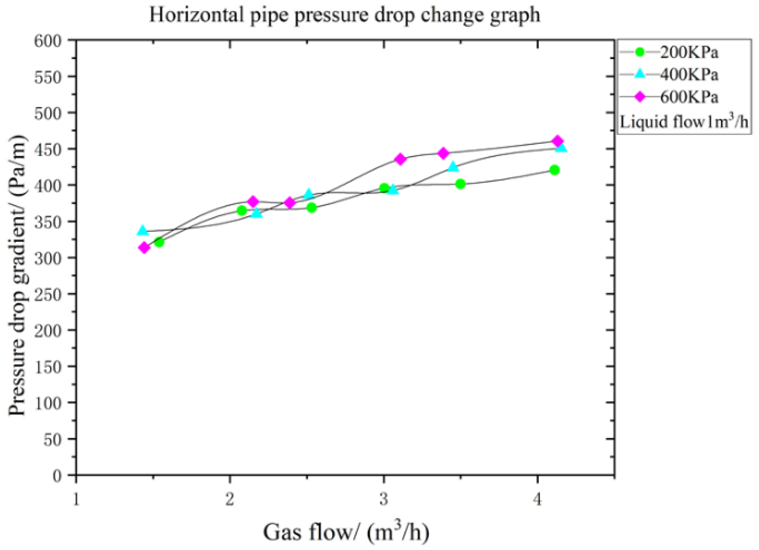
5.1.1. Variation of Pressure Drop under Different Flow Rates

According to the experimental data, the pressure drop change curve of the horizontal pipe under different pressures is drawn, and the influence of different factors on the pressure drop change law is analyzed. Figure 14 presents a graph of pressure drop under different pressures and gas flows. The figure indicates that the overall pressure drop increases with the gas flow rate. Furthermore, the gas velocity increases with the gas flow rate. The frictional resistance between the gas and the pipe wall and between the gas and the liquid increases, thereby increasing the pressure drop gradient.

5.1.2. Horizontal Pipe Pressure Drop Calculation Model

The friction coefficient changes after the foaming agent and the foam stabilizer are added to the water. Using the experimental results, a new calculation and the fitting of the friction coefficient are performed. According to the Beggs–Brill pressure drop programming method, the new friction coefficient expression is obtained as:

$$\lambda =3.681\times {10}^{-10}R{e}^{\prime }{}^2-3.169\times {10}^{-5}R{e}^{\prime }+1.096$$

(2)

$$-\frac{dp}{dz}=\frac{\left[{\rho }_l{H}_l+{\rho }_g\left(1-H_l\right)\right]gsin\theta +\frac{\lambda Gv}{2DA}}{1-\left(\left[{\rho }_l{H}_l+{\rho }_g\left(1-H_l\right)\right]v{v}_{sg}\right)/P}$$

(3)

By substituting the experimental parameters into the above formula, the calculated result is compared with the actual pressure drop, and the total error is less than 6%, proving that this formula is suitable for the current conditions.

5.2. Research on the Resistance of Inclined Upward Pipe

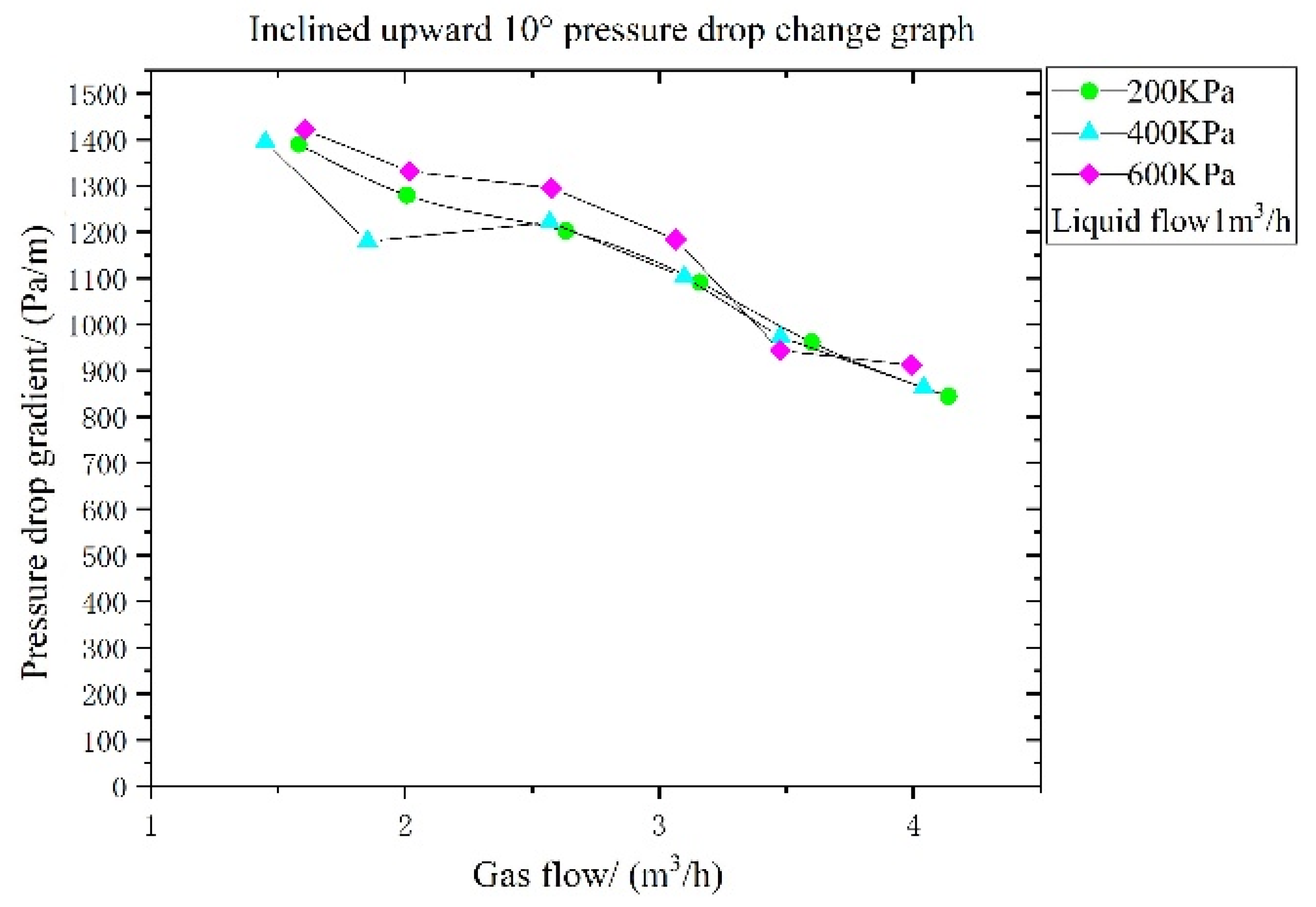
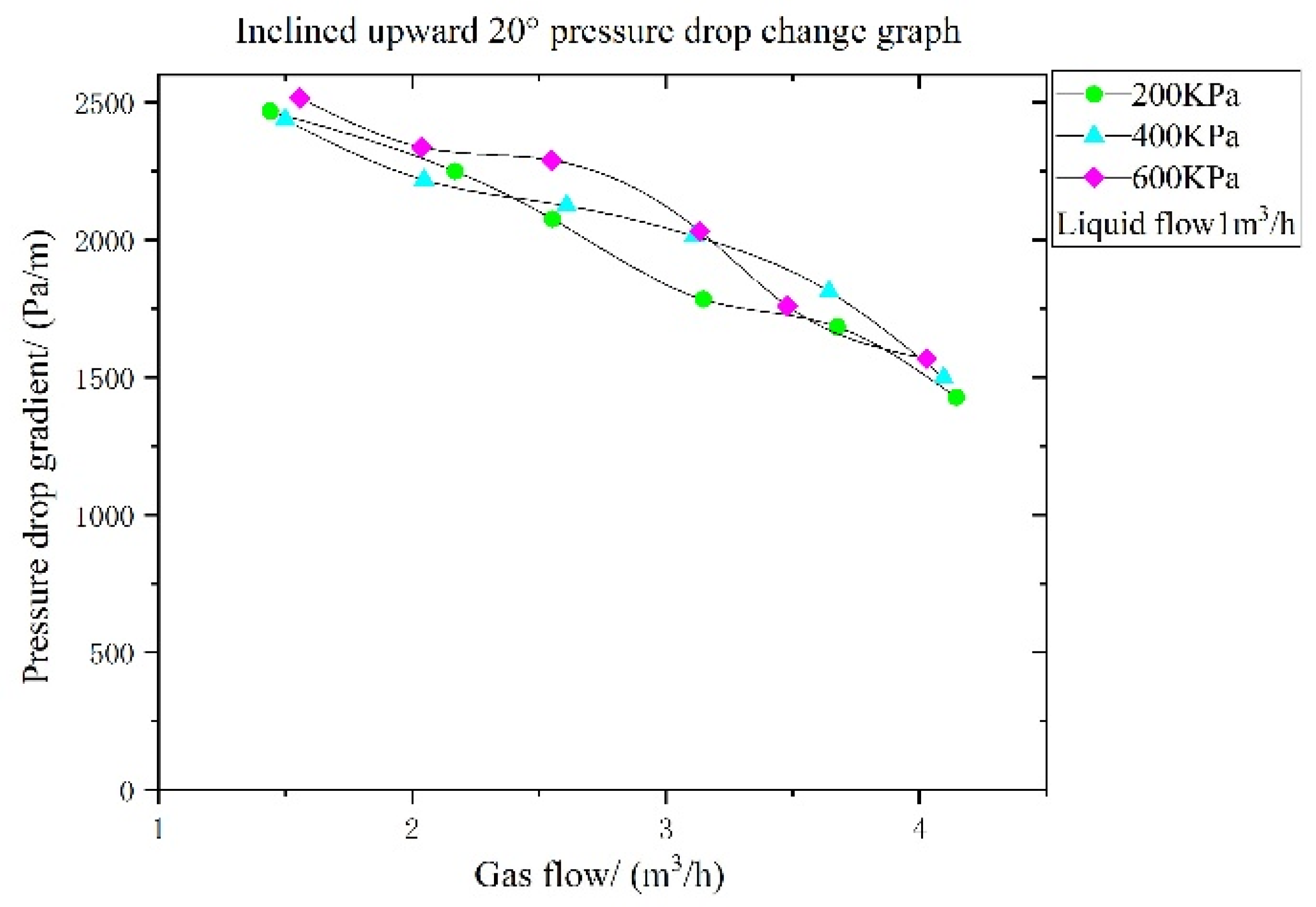
5.2.1. Variation of Pressure Drop under Different Flow Rates

Figure 15 presents a graph of pressure gradients at different pressures and gas flows when tilted upward by 10°, and Figure 16 presents a graph of pressure gradients at different pressures and gas flows when tilted upward by 20°. The figure shows that with the increase in the gas flow rate, the pressure drop gradient decreases with the increase in the gas flow velocity.

When the pipeline is inclined upward, the pressure drop is affected by the gravity position, so the pressure drop is very large. The impact of the pressure drop of the gravity position increases with the angle, so the pressure drop of the pipeline inclined upward by 10° is less than that when the pipeline is inclined upward by 20°. The gas content in the pipeline inclined upward increases with the gas flow, and the mixture density decreases when the gas flow decreases, so the pressure drop will decrease. The corresponding mixture flow speed increases with the gas flow rate, but at this time the pressure drop is the main influencing factor, and the friction pressure drop is the secondary factor.

5.2.2. Inclined Upward Pressure Drop Calculation Model

On the basis of the calculation of the homogeneous flow model, the friction resistance coefficient and the pressure drop formula are fitted using the existing experimental data. After calculation, the new friction coefficient is:

$${\lambda }^{\prime }=\lambda \times 25.887-0.5048$$

(4)

By substituting the experimental parameters into the above formula, the calculated result is compared with the actual pressure drop, and the total error is less than 9%, proving that this formula is suitable for the current conditions.

6. Conclusions

In this research, the change in flow pattern under different initial conditions and the change characteristics of resistance were studied through experiments. Through the experiments, the flow patterns in horizontal and upward-inclined tubes were obtained. The variation of resistance in the tube under different gas–liquid conditions was obtained. However, it is only applicable when the liquid flow does not exceed 1 m³/h and the gas flow does not exceed 4 m³/h. The main conclusions are as follows:

(1)

The comparison of the PDF diagrams obtained using stainless steel pipes and transparent tubes reveals that as long as the gas–liquid flow rate remains unchanged, the shape of the PDF remains basically unchanged in both stainless steel and transparent tubes. Meanwhile, the comparison of the image recognition results and the PDF determines the flow pattern under the gas and liquid flow rates.

(2)

Aiming at the actual operating range of the gas and liquid parameters in the existing application of air foam flooding, gas–water two-phase flow pattern experiments with a foaming agent were conducted. The results show that when the liquid and flow rates do not exceed 1 and 4 m³/h, respectively, in the horizontal pipe, the flow pattern at this time is stratified flow. The flow pattern is slug flow when the pipeline is inclined upward by 10° and 20°, the experimental liquid flow does not exceed 1 m³/h, and the gas flow does not exceed 4 m³/h.

(3)

According to the experimental results, in the case of horizontal pipelines, the pressure drop increases with the gas flow rate. Under the same gas–liquid flow, the pressure drop increases with the pipeline pressure. When the pipeline is inclined upward, the pressure drop will increase with the inclination angle under the same pressure and gas–liquid flow. At the same tilt angle, as the pressure increases, the pressure drop will increase with the gas flow, and the pressure drop will decrease.

(4)

On the basis of the experimental results, this paper establishes the calculation correlation equations for the gas–liquid two-phase flow resistance and the pressure drop in the horizontal and upward-inclined pipes. Compared with the experiment, the error result of the calculation is small. Therefore, under this condition, it can be used to predict the flow resistance in real air foam flooding. In this paper, the research on two-phase flow resistance with foam has expanded the research direction of two-phase flow. In addition to obtaining the resistance variation rule, it can also play a guiding role in the future process design of air foam flooding. However, there are some limitations in this experiment. The length of the pipeline in the experimental section is short, which is quite different from the length of the pipeline in the actual production process. We will carry out the corresponding measurement in the future actual production process to verify and modify the established resistance prediction model.

References

1. Lang, L.; Li, H.; Wang, X.; Liu, N. Experimental study and field demonstration of air-foam flooding for heavy oil EOR. J. Pet. Sci. Eng. 2019, 185, 106659. [Google Scholar] [CrossRef]
2. Liu, P.; Zhang, X.; Wu, Y.; Li, X. Enhanced oil recovery by air-foam flooding system in tight oil reservoirs: Study on the profile-controlling mechanisms. J. Pet. Eng. 2017, 150, 208–216. [Google Scholar] [CrossRef]
3. Zhang, C.; Wang, P.; Song, G. Study on enhanced oil recovery by multi-component foam flooding. J. Pet. Sci. Eng. 2019, 177, 181–187. [Google Scholar] [CrossRef]
4. Fried, A.N. The Foam Drive Process for Increased Recovery of Oil; Report #5866; United States Bureau of Mines: Washington, DC, USA, 1961.
5. Bernard, G.G.; Holm, L.W. Effect of Foam on Permeability of Porous Media to Gas. Soc. Pet. Eng. J. 1964, 4, 267–274. [Google Scholar] [CrossRef]
6. Jensen, J.A.; Fried, F. Physical and chemical effects of an oil phase on the propagation of foam in porous media. Soc. Pet. Eng. 1987. [Google Scholar] [CrossRef]
7. Telmadarreie, A.; Trivedi, J. Insight on Foam/Polymer Enhanced Foam Flooding for Improving Heavy Oil Sweep Efficiency. In Proceedings of the World Heavy Oil Congress 2015, Edmonton, AB, Canada, 24–26 March 2015. [Google Scholar]
8. Telmadarreie, A.; Trivedi, J.J. Post-Surfactant CO2 Foam/Polymer-Enhanced Foam Flooding for Heavy Oil Recovery: Pore-Scale Visualization in Fractured Micromodel. Transp. Porous Media 2016, 113, 717–733. [Google Scholar] [CrossRef]
9. Manan, M.A.; Farad, S.; Piroozian, A.; Esmail, M.J.A. Effects of Nanoparticle Types on Carbon Dioxide Foam Flooding in Enhanced Oil Recovery. Pet. Sci. Technol. 2015, 33, 1286–1294. [Google Scholar] [CrossRef]
10. Bayat, A.E.; Rajaei, K.; Junin, R. Assessing the effects of nanoparticle type and concentration on the stability of CO2 foams and the performance in enhanced oil recovery. Colloids Surf. A Phys. Eng. Asp. 2016, 511, 222–231. [Google Scholar] [CrossRef]
11. San, J.; Wang, S.; Yu, J.; Liu, N.; Lee, R. Nanoparticle-Stabilized Carbon Dioxide Foam Used in Enhanced Oil Recovery: Effect of Different Ions and Temperatures. Spe J. 2017, 22, 1416–1423. [Google Scholar] [CrossRef]
12. Singh, R.; Mohanty, K.K. Study of Nanoparticle-Stabilized Foams in Harsh Reservoir Conditions. Transp. Porous Media 2018, 131, 135–155. [Google Scholar] [CrossRef]
13. Ewing, M.E.; Weinandy, J.J.; Christensen, R.N. Observations of Two-Phase Flow Patterns in a Horizontal Circular Channel. Heat Transf. Eng. 1999, 20, 9–14. [Google Scholar]
14. Weisman, J.; Duncan, D.G.J.C.T.; Gibson, J.; Crawford, T. Effects of fluid properties and pipe diameter on two-phase flow patterns in horizontal lines. Int. J. Multiph. Flow 1979, 5, 437–462. [Google Scholar]
15. Weisman, J.; Kang, S.Y. Flow pattern transitions in vertical and upwardly inclined lines. Int. J. Multiph. Flow 1981, 7, 271–291. [Google Scholar] [CrossRef]
16. Kokal, S.L.; Stanislav, J.F. An experimental study of two-phase flow in slightly inclined pipes—I. Flow patterns. Chem. Eng. Sci. 1989, 44, 665–679. [Google Scholar] [CrossRef]
17. Rafalko, G.; Mosdorf, R.; Gorski, G. Two-phase flow pattern identification in minichannels using image correlation analysis. Int. Commun. Heat Mass Transf. 2020, 113, 104508. [Google Scholar] [CrossRef]
18. Do Amaral, C.E.; Alves, R.F.; da Silva, M.J.; Arruda, L.V.; Dorini, L.; Morales, R.E.; Pipa, D.R. Image processing techniques for high-speed videometry in horizontal two-phase slug flows. Flow Meas. Instrum. 2013, 33, 257–264. [Google Scholar] [CrossRef]
19. Cely, M.M.H.; Baptistella, V.E.; Rodriguez, O.M. Study and characterization of gas-liquid slug flow in an annular duct, using high speed video camera, Wire-Mesh Sensor and PIV. Exp. Fluid Sci. 2018, 98, 563–575. [Google Scholar] [CrossRef]
20. Wang, J.; Lu, T.; Deng, J.; Liu, Y.; Lu, Q.; Zhang, Z. Experimental investigation on pressure oscillation induced by steam lateral injection into water flow in a horizontal pipe. Int. J. Heat Mass Transf. 2019, 148, 119024. [Google Scholar] [CrossRef]
21. Rodrigues, R.L.; Cozin, C.; Naidek, B.P.; Neto, M.A.M.; da Silva, M.J.; Morales, R.E. Statistical Features of the Flow Evolution in Horizontal Liquid-Gas Slug Flow. Exp. Fluid Sci. 2020, 119, 110203. [Google Scholar] [CrossRef]
22. Orkiszewski, J. Predicting Two-Phase Pressure Drops in Vertical Pipe. J. Pet. Technol. 1967, 19, 829–838. [Google Scholar] [CrossRef]
23. Beggs, D.H.; Brill, J.P. A Study of Two-Phase Flow in Inclined Pipes. J. Pet. Technol. 1973, 25, 607–617. [Google Scholar] [CrossRef]
24. Imamura, Y.; Yamada, H.; Ikushima, T.; Shakutsui, H. Pressure Drop of Gas-Liquid Two-Phase Flow in a Large Diameter Vertical Pipe. Res. Mem. Kobe Tech. Coll. 2006, 44, 19–24. [Google Scholar]
25. Hayashi, K.; Kazi, J.; Yoshida, N.; Tomiyama, A. Pressure drops of air-water two-phase flows in horizontal U-bends. Int. J. Multiph. Flow 2020, 131, 103403. [Google Scholar] [CrossRef]
26. Bhagwat, S.M.; Ghajar, A.J. A flow pattern independent drift flux model based void fraction correlation for a wide range of gas–liquid two phase flow. Int. J. Multiph. Flow 2014, 59, 186–205. [Google Scholar] [CrossRef]
Figure 1. Schematic of experimental device.
Energies 14 03722 g001
Figure 2. Image after image processing of stratified flow when the pressure is 0.15 MPa.
Energies 14 03722 g002
Figure 3. Image after image processing of stratified flow when the pressure is 0.2 MPa.
Energies 14 03722 g003
Figure 4. Probability density function diagram at different pressures in horizontal pipeline.
Energies 14 03722 g004
Figure 5. Probability density function of horizontal pipe minus pipe pressure.
Energies 14 03722 g005
Figure 6. Image after image processing when the pressure is 0.15 MPa and tilted upward by 10°.
Energies 14 03722 g006
Figure 7. Image after image processing when the pressure is 0.2 MPa and tilted upward by 10°.
Energies 14 03722 g007
Figure 8. Probability density function of inclined upward by 10°.
Energies 14 03722 g008
Figure 9. Probability density diagram of pipe pressure minus pipe pressure when inclined upward by 10°.
Energies 14 03722 g009
Figure 10. Image after image processing when the pressure is 0.15 MPa and tilted upward by 20°.
Energies 14 03722 g010
Figure 11. Image after image processing when the pressure is 0.2 MPa and tilted upward by 20°.
Energies 14 03722 g011
Figure 12. Probability density function of inclined upward by 20°.
Energies 14 03722 g012
Figure 13. Probability density diagram of pipe pressure minus pipe pressure when inclined upward by 20°.
Energies 14 03722 g013
Figure 14. Pressure gradient diagram under different pressures and gas flows.
Energies 14 03722 g014
Figure 15. Pressure gradient diagram at different pressures and gas flow rates at 10° upward tilt.
Energies 14 03722 g015
Figure 16. Pressure gradient diagram at different pressures and gas flow rates at 20° upward tilt.
Energies 14 03722 g016