Absorption Power and Cooling Combined Cycle with an Aqueous Salt Solution as a Working Fluid and a Technically Feasible Configuration

Abstract

Combined systems for power production and thermally activated cooling have a high potential for improving the efficiency and utilisation of thermal systems. In this regard, various configurations have been proposed and are comprehensively reviewed. They are primarily based on absorption systems and the implementation of multiple levels of complexity and flexibility. The configuration of the absorption power and cooling combined cycle proposed herein has wide commercial applicability owing to its simplicity. The configuration of the components is not new. However, the utilisation of aqueous salt solutions, the comparison with ammonia chiller and with absorption power cycles, the focus on parameters that are important for real-life applications, and the comparison of the performances for constant heat input and waste heat recovery are novel. The proposed cycle is also compared with a system based on the organic Rankine cycle and vapour compression cycle. An investigation of its performance proves that the system is suitable for a given range of boundary conditions from a thermodynamic standpoint, as well as in terms of system complexity and technical feasibility. New possibilities with regard to added power production have the potential to improve the economics and promote the use of absorption chiller systems.

1. Introduction

With increasing environmental awareness, the sustainable use of primary resources, the introduction of renewable energy sources, improvements in the fields of energy efficiency, and lowering the dependency on fossil fuel imports are being pursued. Utilisation of low temperature and waste heat resources, especially at a temperature of approximately 100 °C and in distributed applications at industrial sites, has considerable untapped potential [1,2,3,4] and could contribute to achieving these energy goals. In the cooling sector, there is pressure to make a transition to natural refrigerants with zero ozone depletion potential and negligible global warming potential and to phase out many current ones [5].

Absorption chillers should offer an answer to both issues, yet their high capital cost and low capacity limit their spread. In order to overcome the current drawbacks, there is extensive research ongoing. On the component level, the crucial and most investigated is the absorber with a complicated phenomenon of simultaneous mass and heat transfer. A review of experimental designs [6] shows that the most common falling film type often suffers a wettability problem worsening absorption performance, therefore non-traditional geometries or other types as adiabatic and bubble absorbers are often considered as more compact and cheaper components can be used. Alternatively, a concept with hydrophobic membrane was proposed [7] for both absorber and desorber, with application especially to compact micro-sized chillers. Demonstration of the entire chiller was presented with absorption and desorption rates higher than in previous studies. The second crucial component, desorber, is commonly of a flooded type where the working solution is boiling and optimisation of this process and overall volume has been performed by [8] for LiBr chiller. The second type, falling film, has as a higher heat transfer coefficient requires a small amount of refrigerant, but it is difficult to control [9]. Except for the mentioned membrane type, a flat plate heat exchanger with a subsequent vapour separator has been explored [10,11]. Due to high pressure drop, they were found suitable for compact solutions with high heat source temperatures. In the system level experimental studies, solar cooling and miniaturisation is the most common application, where for example 4.5 kW air cooled LiBr chiller with flat plate collectors achieved a COP of 0.53 while at ambient temperatures above 30 °C managed to chill water to 14 °C [12]. A similar 6 kW chiller with evacuated tube collectors has shown large performance variation with ambient air and chilled water outlet temperature, could achieve a seasonal average COP of about 0.6. The average electrical COP of the entire system was no less than a third of a simple vapour compression system.

If the absorption chiller could provide another product when the cooling load is not required, the improved capacity would boost its economic performance and widen its application. The transformation of primary energy resources for the generation of more than one product can be beneficial because it increases resource utilisation. It may also help to adjust the system products depending on the current needs of customers. Cogeneration of electricity with a by-product of heat (combined heat and power, or CHP) is a well-known concept. However, other cogeneration options are increasingly attracting attention, such as combined cooling and power (CCP) and trigeneration—combined cooling, heat, and power (CCHP). Electricity, heat, and cooling are three products that have different significances depending on the season, ambient temperature, and other factors, while all are often consumed at the same site. A combination of power production and cooling appears to be a suitable and beneficial step.

The cooling effect in cogeneration is, in most concepts, added to the system by thermally activated chillers that process the heat input using absorption, adsorption, desiccant cooling, and other technologies [13,14]. Sorption systems are the only thermally activated systems considered in many studies, and a combination of standalone absorption chillers with different power cycles as the prime mover is the most common [15,16,17]. Looking at the options of absorption cycles, different levels of integration and combination for CCP have been examined in previous studies, including a comprehensive review [18,19]. It shows a wide range of cycle complexity; in some cases, pursuing theoretical improvement in performance makes it difficult for the system to be built and operated. The literature also offers several possibilities on how to assess and compare the performances of power production and chiller heat duty because the two are typically in a different order. The solution was typically found using a weight factor between the two. The systems utilised a water–ammonia mixture as a working fluid with only a few exceptions, such as mixtures of ammonia and lithium nitrate or of ammonia and sodium thiocyanate.

Ejector cooling can be used as well for thermally activated chillers in CCP systems [20], where one subcycle is used to obtain the driving force of the ejector, thus creating a vacuum and cooling in the other subcycle. Then, the work potential does not need to run only the ejector. It can be converted to useful power in the expander, which is then used for running a compressor in a standard vapour compression chiller as in a previous study [21], thus combining the power cycle and compressor chiller into a thermally activated chiller.

The range of the CCP systems based on thermodynamic cycles found in the literature, regardless of the often high level of complexity, can be classified into four main categories based on the general working principle. These categories, outlined in Figure 1 with illustrative T-s diagrams and examples, are as follows:

• Separate thermodynamic cycles coupled by heat
• Separate thermodynamic cycles coupled by work
• Single-branch thermodynamic cycle for both power and thermally activated cooling
• Branched thermodynamic cycle for either power or thermally activated cooling

1.1. Separate Thermodynamic Cycles Coupled by Heat

A thermally activated cooling cycle can be used as a bottoming cycle in the cogeneration configurations schematically shown in Figure 1a. Almost any power cycle can be used as the topping cycle, as long as the heat rejected at a sufficient temperature level can drive thermally activated cooling. Therefore, this system is feasible for a higher heat source temperature. This configuration is beneficial when commercially available power production systems and absorption chillers are combined. Studies have typically focused on overall performance, annual utilisation of power, cooling and heating, economic performance, and optimal control regimes for maximal utilisation of products [13,15,16,17,22,23,24]. The coefficient of performance (COP) of the chiller is typically around 0.7 (in the case of a typical single-effect absorption chiller), while the efficiency of power production depends on the heat source temperature and type of topping cycle(s).

The cycles can also be more integrated, as the utilisation of only a part of rejected heat from compressor intercooling [25] or as a complex set of recuperation heat exchangers in a combination of the Kalina power cycle and bottoming H₂O–LiBr absorption chiller [26,27], which is depicted as the example in Figure 1a. The benefits of such integrated systems are typically an improvement in overall efficiency and a possible reduction in cogeneration annual costs.

1.2. Separate Thermodynamic Cycles Coupled by Work

Power and cooling cycles can be coupled by produced work instead of heat, as illustrated in Figure 1b. In this review, three forms are differentiated: mechanical work, electricity, and motion of the fluid in ejector cooling.

Mechanical and electrical coupling of the systems is primarily considered as a combination of existing technologies. Studies have often focused on the overall performance or experimental validation. In an experimental study on mechanical coupling and application of a motor generator [28], a 1 kWe experimental solar energy system based on an organic Rankine cycle (ORC) and vapour compression cycle (VCC) was constructed using mainly the off-the-shelf components. The unit used a 93 °C heat source and exhibited a chiller regime COP of 0.71, similar to absorption chillers. The authors of the aforementioned study stated that greater benefits could be achieved with higher-temperature heat sources. A similar system was explored in another study [29], although with a fixed mechanical coupling of the expander and compressor. Thus, no power could be produced; nevertheless, the resulting COP was less than 0.6. A specific case of cycle combinations for trigeneration from waste heat has been reported [30], where an additional absorption chiller is used between the ORC and VCC to ensure that the condenser of the VCC remains at a lower temperature. All the systems were coupled electrically, which provides flexibility, making a purely power or cooling regime possible. The system had a COP of 0.2 and a thermal efficiency of 57%. For electricity production, the efficiency was 6%.

Figure 1. Schematic process diagrams of CCP systems with: (a) two separate cycles coupled by heat (example redrawn from [26]), (b) two separate cycles coupled by work (example redrawn from [31]), (c) single-branch thermodynamic cycle (example redrawn from [18]), and (d) two-branch thermodynamic cycle (example redrawn from [32] ).

Figure 1. Schematic process diagrams of CCP systems with: (a) two separate cycles coupled by heat (example redrawn from [26]), (b) two separate cycles coupled by work (example redrawn from [31]), (c) single-branch thermodynamic cycle (example redrawn from [18]), and (d) two-branch thermodynamic cycle (example redrawn from [32] ).

This concept can be simplified using the same working fluid and condenser for both cycles. Such a solar ORC–VCC system was proposed [33] with an expander, compressor, and generator on the same shaft so that electricity or cooling loads can be preferred. Additionally, in winter, the condenser heat can be used for heating in a heat pump regime. A recuperator can also be added to the ORC and VCC to improve the efficiency, thus, the COP, for example, up to 0.66 [27]. Other researchers considered similar systems with combined condensers but without the generator and electricity output. A piston expander–compressor unit proposed in [34] (COP between 0.1 and 0.6, based on the heat source temperature and working fluid) or an ORC heat pump [21] can serve as examples. For a more detailed summary of ORC–VCC systems, the reader is referred to a previous report [33].

The ejector cycles can be combined with power production cycles in several configurations. The simplest and most flexible configuration is a parallel configuration, where the steam at the boiler outlet is routed between the expander and ejector based on the required share between the two products. The vacuum port of the ejector is then connected to the evaporator of the chilling circuit, as shown in Figure 1b. The simplicity of such a system allowed for experimental verification of a small system with cooling capacity up to 5 kW and electrical output up to 1.5 kW (COP around 0.3, electricity production 3% to 4%) [31]. When the heat source temperature and vapour generator pressure are higher than needed for the ejector, extraction turbines have been proposed with the vapour extraction fit for the ejector [35,36]. Another option is to design the expander operating between the vapour generator pressure and optimal ejector driving pressure so that these two are connected serially [37,38,39], where flexibility between the products is, however, lost. To maximise the theoretical output, more complex configurations have also been proposed and investigated [40].

1.3. Single-Branch Thermodynamic Cycle for Both Power and Thermally Activated Cooling

Absorption cycles can be designed in such a way that a vapour stream exiting the vapour generator is used first for power production and then for cooling, as in Figure 1c. The most commonly considered is the Goswami cycle and its modifications, which have been theoretically explored in numerous works [41,42,43,44,45,46,47,48,49,50]. This cycle is based on a simple absorption power cycle (APC) with the utilisation of subambient temperatures at the expander outlet, thus providing a small amount of additional cooling on top of the produced power (typically one third of the turbine work as cooling output). Water–ammonia mixture is considered almost exclusively with only a few exceptions [44,51,52], that operate with different working fluids, such as amyl acetate, propane–decane, or isobutane–decane. The advantage of the Goswami cycle is its simplicity, which utilises an additional heat exchanger added at the expander outlet, because its temperature can be below the ambient temperature. Among the disadvantages are the pressure loss at the vapour side or limited control of the chiller output parameters. The cycle has a fixed chiller output-to-power ratio with a rather low share of cooling, the performance of which depends highly on ambient conditions and expander efficiency.

The Goswami cycle with ammonia has been experimentally explored on a laboratory-scale system with an expander power output of approximately 50–100 W at a nominal vapour generator temperature of 85 °C using a water–ammonia mixture [14,53,54]. At this small scale, owing to thermal losses and low expander efficiency, it was nearly impossible to obtain a subambient temperature at the expander outlet.

Among the modifications of the Goswami cycle, a recuperator has been proposed between the outlet of the expander and evaporator to boost the cooling performance [55]. Other configurations suggested add a condenser after the turbine, effectively splitting the pressure potential by the saturation temperature to reject the heat [56]. Turbine work is partially limited, but the cooling load can be ensured. This concept with an added condenser was suggested not only for the water–ammonia mixture but also for an LiBr–water solution [57]. The cooling load can be further boosted by adding a flashing tank to the stream of the returning solution, thus routing more vapour to the condenser [58].

1.4. Branched Thermodynamic Cycle for Either Power or Thermally Activated Cooling

Finally, the components of the APC and absorption chiller can be arranged into two branches, as illustrated in Figure 1d. The simple form of the cycle shown as an example corresponds to the proposal in an earlier work [59]. This configuration provides very high flexibility because the splitter can freely specify the ratio of vapour passing to the expander or chiller branch. When a water–ammonia mixture is used, a rectifier is typically considered for improved performance, even for simple configurations [60]. Such a system has been experimentally analysed [61], providing a chiller regime COP of approximately 0.6 from a 133 °C temperature of the generated vapour. The expander was only simulated using only an orifice. Several authors have proposed the addition of a superheater upstream of the expander to improve its performance [62] and change the configuration to a generator–absorber–exchanger (GAX) cycle for higher heat source temperatures, as other studies [60,63], or with a separate boiler for turbine and vapour generator [64]. In addition to the water–ammonia mixture, a mixture of ammonia and salts, such as LiNO3 or NaSCN, has been proposed [62,65], where the configurations are simplified by omitting the rectifier. In the simplest configuration, this system was also proposed for the water–LiBr solution, giving a brief idea of the expected parameters [32].

An alternative approach for the water–ammonia system is to route all purified ammonia from the rectifier into the chiller branch of the system. The lean stream of ammonia is then fully evaporated in a separate boiler, and the vapour is fed to the expander and follows as lean input into the absorber [66,67,68]. However, this approach does not allow for control of the ratio between cooling and power. The opposite approach to the cycle configuration [69] excludes the rectifier and routes vapour from the generator into a turbine. The lean solution is flashed at an intermediate pressure, and the vapour is condensed and throttled to the evaporator in the chiller branch.

1.5. Prospects for Aqueous Salt Solution Systems

An aqueous solution of several salts, but mainly LiBr, has been widely used for absorption chillers, especially when a low-temperature heat source is available and chilled temperatures above 0 °C (refrigerant is water) are required. Such a working fluid is environmentally friendly and has low toxicity. Overall, the low pressure level of the system results in fewer legal requirements for installation [70]. However, absorption chillers cost more than double the vapour compression chillers and more expensive is also auxiliary equipment [71]. For example, only less than 2000 of solar absorption cooling systems are installed annually worldwide [72], which also confirms our experience that absorption chillers are not widely used when the cooling load is required only temporarily, mainly because of economic reasons.

Absorption cycles used solely for power production typically adopt an H₂O–NH₃ and are known as ‘Kalina cycles’. They have been the focus of many researchers, as can be seen in several works [73,74,75,76,77]. Newer approaches to APCs also consider other working fluids [78,79,80], where alcohol mixtures of aqueous salt solutions are particularly promising. The salt solutions for power cycles mainly utilise LiBr [32,80,81,82,83], but other salts, such as LiCl or CaCl₂ [78] or LiBr:ZnBr:CaBr2 mixture [84] have been proposed. When applied to low-temperature heat sources at approximately 100 °C, i.e., a domain of single-effect LiBr chillers, these APCs have shown superior performance to ORC with respect to cycle efficiency and utilisation efficiency referenced to the heat source. It was also found that these APCs are more suitable for small distributed energy systems rather than large-scale systems, among others, because of low pressures and associated large volumetric flows of vapour. Therefore, an efficient turbo-expander can also be designed for systems with a small power output [85,86].

As one of thermodynamic cycles with two branches, the absorption combined power and cooling cycle (APCC) using an aqueous salt solution (Figure 1d) can enable a potentially beneficial variability in the power and chiller output, allowing for higher annual utilisation of absorption system. Technical implementation of this system has not indicated any major obstacles. Regardless of the apparent advantages, a detailed analysis of this system has not been reported in the literature. Hence, in this study, the performance of this system is analysed with three salt solutions: LiBr, LiCl, and CaCl₂. The performance is compared with that of a reference system based on ORC and VCC, which represents a system utilising technologies readily available on the market, as well as a system based APCC with same layout and the water–ammonia mixture.

2. Methods

A thermodynamic model was set up for the proposed APCC with a range of investigated working fluids and specified boundary conditions. The same procedure was performed for the reference ORC–VCC system. Performance indicators were considered primarily from the perspective of prospective customers. Application to closed-loop heat source types (cycle efficiency is essential), as well as an open loop for waste heat recovery (utilisation efficiency and absolute output values are essential), was considered in the reported parameters. Additionally, the effect of power consumption of auxiliary systems for heat rejection, an important but often neglected parameter, is included. It is reflected by considering a power requirement of a heat rejection fan. Aiming at high clarity and illustrative value of the results, other parasitic loads are not included in this analysis.

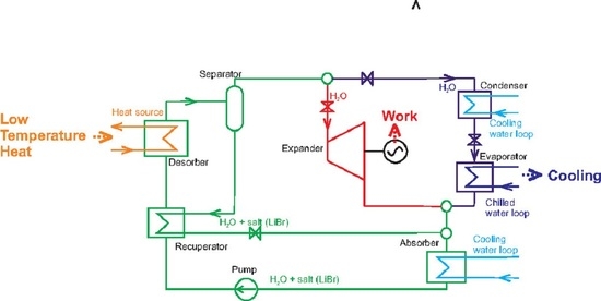
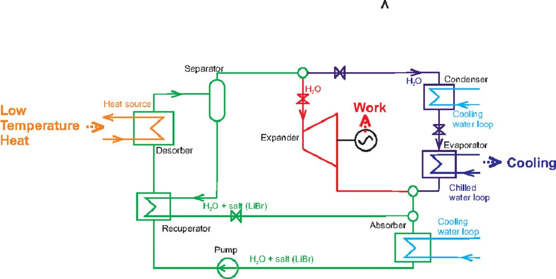
2.1. Proposed Cycle Configuration

A schematic diagram of the proposed APCC (the same for all fluids) is shown in Figure 2. The two-branch arrangement of the cycle is characterised by a separate power branch that corresponds to underscored state in the cycle 1-2-3-4-5-6-7-12-16-17 and by a separate chiller branch that goes through underscored states in the cycle 1-2-3-4-5-8-9-10-11-12-16-17. Apart from this modification, the cycle includes the typical components of the absorption cycle, where the LiBr-rich solution passes through a liquid loop 1-2-3-4-13-14-15-16-17. The configuration is identical to that of the absorption chillers, just with the added power branch.

The lean solution at pressurised liquid state 1 is preheated in the recuperator to state 2, where it is close to its liquid saturation point. This solution enters the desorber, providing heat input into the cycle, reaches the saturated liquid temperature (state 3 within the exchanger), and is partially vaporised. During this isobaric process, part of the more volatile substance (water for a salt solution, NH₃ in the H₂O–NH₃ system) evaporates, and the liquid solution becomes more concentrated by the less volatile one. After the end of heat addition process 4, the steam at state 5 is separated from the liquid at state 13. A splitter divides the steam flow into two branches based on the required ratio between power and cooling, defined by the splitting ratio SR. In the chiller loop, the vapour is first condensed (states 8 and 9), and the condensed water is throttled and evaporated in an evaporator to produce a cooling effect. The low-pressure steam then joins the flow from the turbine in state 12. This low-pressure steam is absorbed into a LiBr-rich liquid from state 15, first adiabatically (steam 16), and then with heat rejection in the absorber until saturated liquid at state 17. The heat rejected in the absorber and condenser is transferred to a water circuit passing through a dry cooling tower.

The reference ORC–VCC system is shown in Figure 3. It consists of an organic Rankine cycle (states 1–8) and VCC (states 11–15). Points not shown in the diagrams correspond to the pinching points within the heat exchangers. To make possible a flexible ratio between the produced work and chiller output, the systems are entirely mechanically decoupled. ORC has a separate generator at the expander, and the vapour compression cycle has a separate motor for the compressor. The ORC utilises R245fa, a typical working fluid for a low-temperature ORC. For the vapour compression cycle, R1234ze(e) was chosen as a typical refrigerant representing new, environmentally friendlier fluids.

2.2. Calculation Method and Boundary Conditions

The models are based on pinch point analysis, which limits the heat transfer in heat exchangers. The following typical assumptions are involved: steady-state operation with the fluid in thermodynamic equilibrium in all nodes, constant isentropic efficiency of components, no heat loss in the components, and no pressure loss (unless specifically mentioned for air in a dry cooling tower). No subcooling is considered at the absorber and condenser outlet, and the effect of varying fluid velocities is neglected. The electrical and mechanical efficiencies are neglected as well.

The system of balance equations of all states accounting for every component is solved using the software Engineering Equation Solver (EES) [87]. One of the most elementary principles used in modelling is the conservation of mass flow and energy for each component, presented in Equations (1) and (2). The working fluid can be a mixture; thus, ${\xi }_{ji}$ represents the ratio of the mass flow of fluid component $j$ to the total mass flow in stream $i$. In the two-phase fluid, the components are evaluated separately for each phase. The term ${\dot{m}}_i$ stands for the mass flow rate in each of the streams i. In Equations (2)–(4), ${\dot{W}}_{pump/comp/fan}$ represents the power of the adequate components, $h_{in}$ is the enthalpy of the working fluid at the inlet of the component and $h_{out,is}$ is the enthalpy at the outlet considering an isentropic process.

$${\displaystyle \sum }_i{\displaystyle \sum }_j{\xi }_{ji}{\dot{m}}_i=0$$

(1)

$$\sum h_i{\dot{m}}_i+\dot{Q}-\dot{W}=0$$

(2)

Rotating components, such as expanders, pumps, compressors, and a fan for a dry cooler, are calculated using isentropic efficiency ${\eta }_{is}$, as shown in Equations (3) and (4). The consumed work (pump, fan) has a negative sign to comply with Equation (2).

$${\dot{W}}_{exp}=\dot{m}\left(h_{in}-h_{out,is}\right) {\eta }_{is}$$

(3)

$${\dot{W}}_{pump/comp/fan}=\dot{m}\left(h_{in}-h_{out,is}\right)/{\eta }_{is}$$

(4)

The cycles are modelled together with secondary fluids for heat input, heat rejection, and chilled water. Heat transfer in heat exchangers is limited by the specified pinch points. The pinch point may be at the heat exchanger inlet or outlet (in the case of the recuperator, evaporator, dry cooler, and, in some regimes, desorber) or at the point when phase change begins (condenser, desorber). However, because of the temperature glide of the working fluid during the phase change, it might have an arbitrary position in the middle of the heat exchanger (absorber). To evaluate the heat exchangers with temperature glide (desorber and absorber) properly, they are discretised into 30 elements, and the mass flow rates in the model are iterated to satisfy the specified pinch points. Because pinch point analysis is implemented, the results represent a set of design points.

In these models, the heat source is considered to be hot (pressurised) water. The heat rejection circuit uses a water loop and dry cooler. The heat transfer and temperature levels are given by the pinch point requirements in all the heat exchangers.

The parameters controlling the APCC are as follows: the chiller branch evaporation temperature $T_{eva}$, concentration of salt or ammonia in the lean solution ${\xi }_1$ (which defines absorber pressure), and temperature at the desorber outlet $T_5$ provided by the pinch point. Another control parameter is required, which can be either a concentration difference between rich and lean solutions (used as optimisation parameters for waste heat recovery applications) or a fixed heat source outlet temperature (i.e., constant heat input, used for baseline analyses).

The ORC–VCC model differs based on the pinch point of the ORC at the point of a saturated liquid. The ORC evaporation temperature is in the baseline case (constant heat input) resulting from the required heat source outlet temperature, whereas, in the case of waste heat recovery, it is an optimisation parameter. The condensing temperature of the ORC is optimised to provide the maximum net power output. The condensing temperature of the VCC is then set to the same value.

Finally, the parameter SR, which determines the ratio of the power and chiller output, is defined. The In the APCC, it provides the ratio between the steam mass flow rate to the expander branch and the steam mass flow at the separator outlet. For the ORC–VCC system, this ratio describes the portion of the expander work used as the power output, while the remaining power is used to drive the VCC compressor.

Fluid properties were taken as inbuilt in EES, particularly the IAPWS-95 [88] formulation for pure water, the water–ammonia mixture properties came from a previous report [89], and the LiCl solution is based on another report [90]. The properties of the H₂O–LiBr solution were taken from the external EES library [91], which is an implementation of a formulation that can be found elsewhere [92]. The properties of the CaCl₂ solution were determined separately using the correlations from earlier work [93]. However, because of the absence of enthalpy, the provided heat capacity and ideal mixing rules were used; thus, caution should be exercised when assessing the results of this fluid.

The boundary conditions of the model that are constant in this analysis are summarised in

Table 1. Boundary conditions of the models.

Tamb	pamb	RHamb	Ths	Teva	T51	ΔTmin, HX
(°C)	(kPa)	(%)	(°C)	(°C)	(°C)	(°C)
25	101.325	70	95	5	15	5
ṁhs	phs	pcw	ΔpDC	ηis	ξsol,1	Ths, out
(kg s−1)	(kPa)	(kPa)	(kPa)	(%)	(%)	(°C)
2.5	8 000	200	0.15	80	56	85

. The values are taken to reflect similar actual systems of absorption chillers [70]. The expander efficiency is taken as a state of the art from micro turboexpander experimental investigations [94,95].

The controlled variables are the temperatures of the heat source fluid $T_{hs}$ (mass flow fixed for all cases) and of ambient air $T_{amb}$, which provide cooling water from the dry cooler after rejecting heat. A higher pressure is used for the heat source water so that it remains liquid for sensitivity analysis with respect to higher heat source temperatures.

2.3. Performance Analysis Methods

Energy and exergy analyses of cogeneration systems in the literature have been performed with various degrees of complexity. A comprehensive approach is to account for primary energy conversion from a global perspective, including a comparison of the average power production efficiency of the electricity from the grid, as proposed for CCP and CCHP cycles by Ayou et al. [18]. The authors of this work, however, believe that in the current state of technology, for a clear assessment of the parameters of the cycle, and from the viewpoints of potential users, manufacturers, and operators, simpler and more-straightforward performance indicators are suitable.

The simple energy efficiency ${\eta }_{cycle}$ is defined using Equation (5), where ${\dot{W}}_{cycle}$ is the net work of the cycle, ${\dot{Q}}_{chill}$ is the chiller output and ${\dot{Q}}_{hs,used}$ is the total thermal input used from the heat source. It can be divided into the efficiency of power production ${\eta }_{cycle,pow}$ and the COP of the chiller $CO{P}_{cycle}$, which are defined in Equations (6) and (7), respectively. The power production efficiency may be negative when the power production drops below zero (W_exp < W_pump) for a higher chiller output.

$${\eta }_{cycle}=\frac{{\dot{W}}_{cycle}+{\dot{Q}}_{chill}}{{\dot{Q}}_{hs,used}}=\frac{{\dot{W}}_{exp}+{\dot{W}}_{pump}+{\dot{Q}}_{chill}}{{\dot{Q}}_{hs,used}}$$

(5)

$${\eta }_{cycle,pow}=\frac{{\dot{W}}_{cycle}}{{\dot{Q}}_{hs,used}}$$

(6)

$$CO{P}_{cycle}=\frac{{\dot{Q}}_{chill}}{{\dot{Q}}_{hs,used}}$$

(7)

When the auxiliary power requirements of the system are considered (here represented by fan power for heat rejection), the formula for power efficiency ${\eta }_{cycle,pow,net}$ changes in its numerator according to Equation (8). The net overall efficiency or COP with respect to the overall energy input is not reported in such a manner because the gross and net power efficiencies already show the difference between the two.

$${\eta }_{cycle,pow,net}=\frac{{\dot{W}}_{net}}{{\dot{Q}}_{hs,used}}=\frac{{\dot{W}}_{cycle}+{\dot{W}}_{fan}}{{\dot{Q}}_{hs,used}}$$

(8)

Exergy efficiency is determined to assess the useful products, work, and cooling output from the perspective of the second law of thermodynamics. For the cycle itself, the exergy efficiency ${\eta }_{ex,cycle}$ is defined by Equation (9), while the net exergy efficiency ${\eta }_{ex,net}$, including that of auxiliary systems, is given by Equation (10). The change in exergy of the heat source $\Delta {\dot{Ex}}_{hs}$ and chilling streams $\Delta {\dot{Ex}}_{chill}$ is represented by Equations (11) and (12), with the states corresponding to Figure 2 and Figure 3. State 0 corresponds to the ambient temperature ($T_0$ in K units); ${\dot{m}}_{cool}$ represents the mass flow rate of the coolant.

$${\eta }_{ex,cycle}=\frac{{\dot{W}}_{cycle}+\Delta {\dot{Ex}}_{chill}}{\Delta {\dot{Ex}}_{hs}}$$

(9)

$${\eta }_{ex,net}=\frac{{\dot{W}}_{net}+\Delta {\dot{Ex}}_{chill}}{\Delta {\dot{Ex}}_{hs}}$$

(10)

$$\Delta {\dot{Ex}}_{chill}={\dot{Ex}}_{cf,out}-{\dot{Ex}}_{cf,in}={\dot{m}}_{cool}\left[\left(h_{52}-h_{51}\right)-T_0\left(s_{52}-s_{51}\right)\right]$$

(11)

$$\Delta {\dot{Ex}}_{hs}={\dot{Ex}}_{hs,in}-{\dot{Ex}}_{hs,out}={\dot{m}}_{hs}\left[\left(h_{21}-h_{23}\right)-T_0\left(s_{21}-s_{23}\right)\right]$$

(12)

In applications with an open-loop heat source (such as waste heat recovery), utilisation efficiency (${\eta }_{util,net}$ for the 1^st law evaluation and ${\eta }_{ex,util, net}$ for the 2^nd law evaluation) is a more important parameter than cycle efficiency. The reference, in this case, is the heat released when the heat source is cooled to the ambient temperature. Therefore, the capability of the cycle to extract heat from the heat source is also considered. This is particularly the area where the cycles with temperature glide should provide an advantage by better matching their Q–T profile to the heat source [96,97]. Efficiency functions, therefore, change the denominator term, as shown in Equations (13) and (14). The utilisation efficiency of power production and COP are analogous to Equations (6)–(8) with ${\dot{Q}}_{hs,all}$ in the denominator.

$${\eta }_{util,net}=\frac{{\dot{W}}_{net}+{\dot{Q}}_{chill}}{{\dot{Q}}_{hs,all}}=\frac{{\dot{W}}_{net}+{\dot{Q}}_{chill}}{{\dot{m}}_{hs} \left(h_{21}-h_{T_0}\right)}$$

(13)

$${\eta }_{ex,util, net}=\frac{{\dot{W}}_{net}+\Delta {\dot{Ex}}_{chill}}{{\dot{Ex}}_{hs}}=\frac{{\dot{W}}_{net}+\Delta {\dot{Ex}}_{chill}}{{\dot{m}}_{hs}\left[\left(h_{21}-h_{T_0}\right)-T_0\left(s_{21}-s_{T_0}\right)\right]}$$

(14)

3. Results and Discussion

First, the overall parameters of the systems are reported for the APCC with the most typical working fluid, the LiBr solution, and for the reference ORC–VCC system. A sensitivity analysis shows the performance with respect to the major inputs. The effect of auxiliary equipment consumption on the net performance is shown, as well as the difference in the results for constant heat input and for an open-loop heat source. Finally, a comparison of the APCC parameters with the optimal parameters of absorption power-only cycles and a comparison of different working fluids are presented.

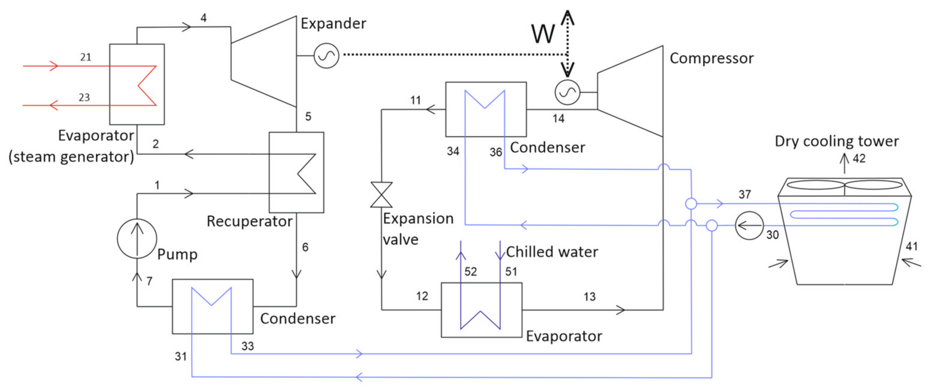
3.1. Baseline APCC and Comparison with VCC–ORC

The parameters of the cycles for the baseline condition, when the heat source outlet temperature is fixed at 85 °C, and the splitting ratio SR has a value of 0.5, as shown in

Table 2. Main resulting parameters of the APCC and ORC–VCC at baseline conditions with SR 0.5.

Parameter	Unit	APCC	ORC–VCC
${\eta }_{cycle}$	%	43.5	24.8
${\eta }_{cycle,pow}$	%	4.24	3.81
$CO{P}_{cycle}$	1	0.39	0.21
${\eta }_{cycle,pow,net}$	%	1.88	1.51
${\eta }_{ex,cycle}$	%	33.3	26.4
${\eta }_{ex,net}$	%	20.1	13.6
${\dot{Q}}_{chill}$	kW	41.3	22.0
${\dot{Q}}_{hs,used}$	kW	105.1	105.1
${\dot{Q}}_{rej}$	kW	141.9	123.1
${\dot{Q}}_{reg}$	kW	43.3	3.0
${\dot{W}}_{exp}$	kW	4.46	8.58
${\dot{W}}_{pump}$	kW	−0.003	−0.29
${\dot{W}}_{comp}$	kW	0	−4.29
${\dot{W}}_{fan}$	kW	−2.48	−2.42
${\dot{W}}_{net}$	kW	1.98	1.58

. Moreover,

Table A1. Parameters of the APCC in its nodes for baseline conditions (imposed values in underscored bold).

Node	T (°C)	p (kPa)	h (kJ kg−1)	ṁ (kg s−1)	s (kJ kg−1 K−1)	ξ (1)	x (1)
1	36.4	8.683	92	0.499	0.221	0.560	subc
2	79.1	8.683	179	0.499	0.484	0.560	subc
3	80.1	8.683	181	0.499	0.490	0.560	0
4	90.0	8.683	389	0.499	1.072	0.560	0.030
5	90.0	8.683	2669	0.035	8.463	0.000	sup
6	90.0	8.683	2669	0.018	8.463	0.000	1
7	5.0	0.8725	2417	0.018	8.689	0.000	0.963
8	90.0	8.683	2669	0.018	8.463	0.000	sup
9	43.1	8.683	180	0.018	0.613	0.000	0
10	5.0	0.8725	180	0.018	0.649	0.000	0.109
11	5.0	0.8725	2510	0.018	9.025	0.000	1
12	5.0	0.8725	2463	0.035	8.857	0.000	0.981
13	90.0	8.683	215	0.463	0.508	0.603	0
14	41.4	8.683	122	0.463	0.231	0.603	subc
15	41.4	0.8725	122	0.463	0.232	0.603	0.017
16	44.7	0.8725	288	0.499	0.847	0.560	0.028
17	36.4	0.8725	92	0.499	0.221	0.560	0
21	95.0	800	399	2.500	1.250
22	85.1	800	357	2.500	1.135
23	85.0	800	357	2.500	1.134
30	30.0	200	126	3.665	0.437
31	30.0	200	126	2.404	0.437
32	39.7	200	167	2.404	0.569
33	30.0	200	126	1.261	0.437
34	38.4	200	161	1.261	0.550
35	39.3	200	164	3.665	0.563
41	25.0	101.3	61	14.860	5.823
42	34.3	101.3	70	14.860	5.855
51	15.0	200	63	1.969	0.224
52	10.0	200	42	1.969	0.151

and

Table A2. Parameters of the ORC-VCC in its nodes for baseline conditions (imposed values in underscored bold).

Node	T (°C)	p (kPa)	h (kJ kg−1)	ṁ (kg s−1)	s (kJ kg−1 K−1)	x (1)
1	43.3	841.7	257	0.524	1.192	subc
2	47.4	841.7	263	0.524	1.210	subc
3	82.5	841.7	313	0.524	1.358	0
4	82.5	841.7	463	0.524	1.781	1
5	53.9	275.3	447	0.524	1.794	sup
6	48.3	275.3	441	0.524	1.776	sup
7	43.0	275.3	436	0.524	1.759	1
8	43.0	275.3	257	0.524	1.192	0
11	35.0	831.5	249	0.158	1.165	subc
12	5.0	261.2	249	0.158	1.174	0.23
13	5.0	261.2	388	0.158	1.674	1
14	45.3	831.5	415	0.158	1.691	sup
15	43.0	831.5	412	0.158	1.682	1
16	43.0	831.5	260	0.158	1.202	0
21	95.0	800	399	2.500	1.250
22	87.5	800	367	2.500	1.163
23	85.0	800	357	2.500	1.134
30	30.0	200	126	3.584	0.437
31	30.0	200	126	2.811	0.437
32	38.0	200	159	2.811	0.546
33	38.2	200	160	2.811	0.549
34	30.0	200	126	0.773	0.437
35	38.0	200	159	0.773	0.546
36	38.2	200	160	0.773	0.548
37	38.2	200	160	3.584	0.549
41	25.0	101.3	61	14.530	5.823
42	33.2	101.3	69	14.530	5.852
51	15.0	200	63	1.052	0.224
52	10.0	200	42	1.052	0.151

list the reported thermodynamic parameters in all the system nodes, where the controlling parameters of the cycles are highlighted in bold. The parameters as concentrations were chosen as typical for absorption chillers and were the baseline parameters for further analyses.

The cycle efficiency is mainly affected by the cooling output, while the exergy efficiency is affected by the power output. This was further demonstrated in the sensitivity analysis. The APCC, in comparison with the ORC–VCC system, provides nearly double chiller capacity while having at the same time an approximately 25% higher net power output. The power requirement of the auxiliary equipment (${\dot{W}}_{fan}$) is similar for both cases.

Figure 4 shows T–s and T–S diagrams (with specific and absolute entropy) of the APCC to provide a clear idea of the processes occurring in the cycle. It can be seen that the recuperated heat and sensible heat input to the solution are large compared with the heat input and heat added for the phase change process. This is caused by a small concentration difference in the solution, which is common for absorption chillers. This is different from the situation of the APC optimised for waste heat recovery [78], where the concentration difference must be significantly larger to obtain a larger temperature glide. As the pressure difference in the absorption cycle is low, the entropy change during throttling or expansion in the diagrams is also considerably small.

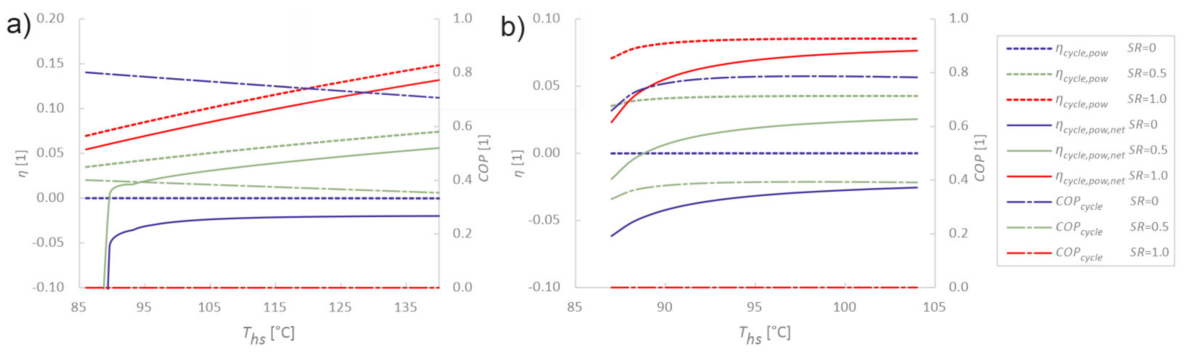
3.2. Sensitivity Analysis of Cycle Parameters

Sensitivity analysis is performed first for the parameters from the cycle perspective (situations with constant heat input and a closed-loop heat source). The following is an analysis performed for operation in waste heat recovery applications, where the goal is to maximise the utilisation efficiency (regardless of cycle efficiency and the amount of heat extracted from the heat source).

The APCC and ORC–VCC are designed for flexible operation with variation between power and cooling output defined by the splitting ratio $SR$, so its impact on the performance indicators is significant and is shown in Figure 5. As expected from the SR definition, all the considered parameters depend linearly on the splitting ratio. However, the results clearly illustrate the disproportion between the quantity and quality of the products—cooling output and electricity. The energy efficiency is largely affected by the cooling output because the absolute value of the electrical output is low. The situation is nearly the opposite for the exergy efficiency. As the exergy of chilled water is rather low, the exergy efficiency is highest when only electricity is produced. The net efficiencies then show the extent of power needed to run the fans. In the regime for the maximum cooling load (SR = 0), the negative net electrical efficiency represents the power consumption of all auxiliary systems. The absolute value is more than half the positive net power production in the purely power-producing regime (SR = 1). The disproportion between the low exergy of the chilled water output and the high exergy of the electrical output then causes low exergy efficiency for the chiller operation. It can even result in negative values for SR between 0 and approximately 0.2. The exergy output of chilled water is, in this case, lower than the required electricity (pure exergy) input.

In the power-only production regime, the absorption cycle has only slightly better performance than the ORC (gross and net power efficiencies of 8.5% and 6.9% for APC against 7.9% and 6.1% for ORC). However, a large difference was observed for the chiller regime with a COP of 0.79 for the absorption system and 0.42 for the ORC–VCC, respectively, while the net power efficiency is nearly the same (−3.2% versus −3.1%). A clear advantage of the absorption system for the combined system is shown.

The difference in the lean and rich concentrations is among the most important controlling parameters of the absorption cycles. Figure 6 shows its impact when the heat source temperature is kept constant, and the concentration difference Δξ is used as an input in the model instead of the outlet temperature of the heat source. As Δξ increases at a nearly constant desorber temperature, the pressure drops. A limit for the high Δξ is the pressure in the condenser so that the condensation temperature is sufficiently high for heat rejection to the ambient. Under the pinch point constraints, a low condenser pressure causes the cooling water and air mass flow rates to increase, similar to the parasitic load. As a result, a sharp decline in the net power efficiency can be seen when the chiller branch is in operation, whereas only a moderate decrease is observed for producing only power. The gross power efficiency has a maximum at a very low Δξ, where the cycle extracts only a small amount of heat from the heat source at high temperature. The net efficiency maximum is at higher values before it declines owing to the low-temperature difference in the condenser and absorber and the associated high parasitic load. The COP increase with Δξ is only moderate, while there is a sharp drop in the net power efficiency after its optimum.

Sensitivity analyses of the heat source temperature (two operating regimes) as well as the ambient and evaporator temperatures agree with the typical behaviour of absorption chillers or power cycles. This can be found in Figure A1 and Figure A2 (in Appendix A).

3.3. Sensitivity Analysis of Utilisation Parameters

To maximise the utilisation of a heat source, fixing its outlet temperature is not suitable. Searching for the optimum is straightforward by varying the specified boiling temperature of the ORC, maximising the net power output of the cycle. The VCC is independent of the ORC. For the APCC, the net power and COP work against each other. The approach adopted in the optimisation is to search for a concentration difference Δξ and lean solution concentration ξ₁, which together provide maximal net power output at SR = 0.5. The resulting parameters for each node for both systems are presented in

Table A3. Parameters of the APCC in its nodes after optimisation for heat source utilisation (imposed values in underscored bold).

Node	T (°C)	p (kPa)	h (kJ kg−1)	ṁ (kg s−1)	s (kJ kg−1 K−1)	ξ (1)	x (1)
1	35.5	8.089	88	0.502	0.218	0.555	subc
2	77.5	8.089	174	0.502	0.479	0.555	subc
3	77.6	8.089	174	0.502	0.479	0.555	0
4	90.0	8.089	435	0.502	1.211	0.555	0.030
5	90.0	8.089	2669	0.045	8.496	0.000	sup
6	90.0	8.089	2669	0.022	8.496	0.000	1
7	5.0	0.8725	2424	0.022	8.715	0.000	0.963
8	90.0	8.089	2669	0.022	8.496	0.000	sup
9	41.7	8.089	175	0.022	0.595	0.000	0
10	5.0	0.8725	175	0.022	0.629	0.000	0.109
11	5.0	0.8725	2510	0.022	9.025	0.000	1
12	5.0	0.8725	2467	0.045	8.870	0.000	0.981
13	90.0	8.089	218	0.458	0.502	0.609	0
14	40.5	8.089	124	0.458	0.224	0.609	subc
15	40.5	0.8725	124	0.458	0.224	0.609	0.017
16	45.9	0.8725	331	0.502	0.993	0.555	0.028
17	35.5	0.8725	88	0.502	0.218	0.555	0
21	95.0	800	399	2.500	1.250
22	82.5	800	346	2.500	1.105
23	82.5	800	346	2.500	1.105
30	30.0	200	126	4.624	0.437
31	30.0	200	126	2.717	0.437
32	40.8	200	171	2.717	0.582
33	30.0	200	126	1.907	0.437
34	37.0	200	155	1.907	0.532
35	39.2	200	164	4.624	0.562
41	25.0	101.3	61	18.750	5.823
42	34.2	101.3	70	18.750	5.855
51	15.0	200	63	2.480	0.224
52	10.0	200	42	2.480	0.151

and

Table A4. Parameters of the ORC-VCC in its nodes after optimisation for heat source utilisation (imposed values in underscored bold).

Node	T (°C)	p (kPa)	h (kJ kg−1)	ṁ (kg s−1)	s (kJ kg−1 K−1)	x (1)
1	43.3	725.7	257	0.905	1.192	subc
2	46.2	725.7	261	0.905	1.205	subc
3	76.6	725.7	304	0.905	1.334	0
4	76.6	725.7	460	0.905	1.777	1
5	52.3	275.3	445	0.905	1.788	sup
6	48.3	275.3	441	0.905	1.776	sup
7	43.0	275.3	436	0.905	1.759	1
8	43.0	275.3	257	0.905	1.192	0
11	35.0	831.5	249	0.237	1.165	subc
12	5.0	261.2	249	0.237	1.174	0.23
13	5.0	261.2	388	0.237	1.674	1
14	45.3	831.5	415	0.237	1.691	sup
15	43.0	831.5	412	0.237	1.682	1
16	43.0	831.5	260	0.237	1.202	0
21	95.0	800	399	2.500	1.250
22	81.6	800	342	2.500	1.094
23	77.9	800	327	2.500	1.050
30	30.0	200	126	3.584	0.437
31	30.0	200	126	4.854	0.437
32	38.0	200	159	4.854	0.546
33	38.2	200	160	4.854	0.549
34	30.0	200	126	1.155	0.437
35	38.0	200	159	1.155	0.546
36	38.2	200	160	1.155	0.548
37	38.2	200	160	6.009	0.549
41	25.0	101.3	61	24.360	5.823
42	33.2	101.3	69	24.360	5.852
51	15.0	200	63	1.571	0.224
52	10.0	200	42	1.571	0.151

(in Appendix A).

The values of utilisation efficiency and COP are shown for both systems in Figure 7. The trends are similar to that of the efficiency with respect to the transferred heat, but the values are significantly lower because the cycles can utilise only a small portion of the heat from the heat source. The APCC again provided a significantly higher COP in the pure chiller regime. Therefore, the overall exergy efficiency is approximately zero for the APCC, whereas it attains negative values for the ORC–VCC owing to the low exergy of the cooling output. The point where the net utilisation efficiency and COP intersect is the point at which the net power output is zero. When the system is used only for power production, the ORC-VCC has a higher efficiency, although only by 0.1%.

Figure 8 shows the impact of the heat source temperature and concentration difference on the utilisation parameters. Because it is fairly common for absorption chillers, increasing the heat source temperature results in a notable decrease in the COP (but a higher cooling capacity from the same heat source mass flow rate). For the power production, the efficiency with the temperature difference increases. The sharp decrease in the net power efficiency at low temperatures is caused by the decreased temperature difference for heat rejection, mainly from the condenser. Therefore, this drop is not observed in the power-only production regime. By varying the concentration difference, the maximum efficiency point of the power-only production was beyond the displayed region. This is explored further in Section 3.5 on the comparison of APCC with APC for power-only production. A higher concentration difference, however, causes a decrease in the desorber and condenser pressure (and, thus, the condensing temperature), limiting the operational possibility of the APCC and increasing the parasitic load, regardless of an increase in the COP. Therefore, for specific applications, optimisation with respect to the required power and cooling output can be performed.

3.4. Comparison of Working Fluids

To compare the results with the possibilities of other working fluids, an investigation was conducted to include an ammonia–water mixture and alternative aqueous solutions with LiCl and CaCl₂, which are also considered for absorption chillers. With ammonia, the combined system has been considered with and without a rectifier, where the rectifier would increase the ammonia concentration from the separator outlet. To provide coherent work with the same layout and system complexity, the basic configuration without the rectifier is considered. The water–ammonia system has a vapour quality at an evaporator outlet lower than one and corresponds to the fluid temperature limit provided by the minimum required temperature difference. The reason is the temperature glide, and the excessively high evaporation temperature after most of the ammonia is already in a vapour form.

The parameters of the concentrations were chosen to agree with the typical values and to provide a reasonable trade-off in performance between the auxiliary (fan) consumption and the cycle performance. The same issue has already been discussed for the LiBr APCC.

Table 3. Main resulting cycle parameters of the different working fluids: salt solutions and water–ammonia mixture.

	ξ1 (1)	ξ2 (1)	p1 (kPa)	p2 (kPa)	SR (1)	$\mathit{C}\mathit{O}{\mathit{P}}_{\mathit{c}\mathit{y}\mathit{c}\mathit{l}\mathit{e}}$ (1)	${\mathit{\eta }}_{\mathit{c}\mathit{y}\mathit{c}\mathit{l}\mathit{e},\mathit{p}\mathit{o}\mathit{w}}$ (%)	${\mathit{\eta }}_{\mathit{c}\mathit{y}\mathit{c}\mathit{l}\mathit{e},\mathit{p}\mathit{o}\mathit{w},\mathit{n}\mathit{e}\mathit{t}}$ (%)	${\mathit{\eta }}_{\mathit{e}\mathit{x},\mathit{c}\mathit{y}\mathit{c}\mathit{l}\mathit{e}}$ (%)	${\mathit{\eta }}_{\mathit{e}\mathit{x},\mathit{n}\mathit{e}\mathit{t}}$ (%)
H2O-LiBr	0.56	0.60	8.7	0.87	0	0.79	0.0	−3.2	19.2	1.5
					0.5	0.39	4.2	1.9	33.3	20.1
					1	0.00	8.5	6.9	47.4	38.8
H2O-LiCl	0.44	0.52	9.1	0.87	0	0.79	0.0	−3.1	19.3	2.2
					0.5	0.40	4.4	2.0	34.0	21.0
					1	0.00	8.7	7.1	48.7	39.7
H2O-CaCl2	0.56	0.68	7.7	0.87	0	0.74	0.0	−3.3	18.2	−0.3
					0.5	0.37	3.8	1.6	30.4	17.9
					1	0.00	7.6	6.5	42.6	36.3
NH3-H2O	0.50	0.45	1512.2	458.6	0	0.56	−0.9	−3.6	8.3	−6.3
					0.5	0.28	3.1	1.0	23.9	12.2
					1	0.00	7.1	5.5	39.6	30.7

lists the results for the major cycle parameters. The performances of the cycles with a salt solution were quite similar. The best chiller performance was achieved using the LiCl solution. The COP was 0.79, which is the same as that of the LiBr solution, which had a slightly higher net power consumption. The highest power production resulted from the LiCl solution. The water–ammonia working fluid provided the poorest performance with an approximately 30% lower COP in chiller operation (partial improvement could be achieved with an added rectifier) and 20% lower net power output.

Table 4. Main resulting utilisation parameters of the different working fluids: salt solutions and water–ammonia mixture.

	ξ1 (1)	ξ2 (1)	p1 (kPa)	p2 (kPa)	SR (1)	$\mathit{C}\mathit{O}{\mathit{P}}_{\mathit{u}\mathit{t}\mathit{i}\mathit{l}}$ (1)	${\mathit{\eta }}_{\mathit{u}\mathit{t}\mathit{i}\mathit{l},\mathit{p}\mathit{o}\mathit{w}}$ (%)	${\mathit{\eta }}_{\mathit{u}\mathit{t}\mathit{i}\mathit{l},\mathit{p}\mathit{o}\mathit{w},\mathit{n}\mathit{e}\mathit{t}}$ (%)	${\mathit{\eta }}_{\mathit{u}\mathit{t}\mathit{i}\mathit{l}}$ (%)	${\mathit{\eta }}_{\mathit{u}\mathit{t}\mathit{i}\mathit{l},\mathit{n}\mathit{e}\mathit{t}}$ (%)	${\mathit{\eta }}_{\mathit{e}\mathit{x},\mathit{u}\mathit{t}\mathit{i}\mathit{l},\mathit{n}\mathit{e}\mathit{t}}$ (%)
H2O-LiBr	0.56	0.61	8.1	0.87	0	0.14	0.0	−0.6	14.2	13.6	0.2
					0.5	0.07	0.7	0.3	7.8	7.4	6.2
					1	0.00	1.5	1.2	1.5	1.2	12.1
H2O-LiCl	0.43	0.52	9.2	0.87	0	0.13	0.0	−0.5	12.5	13.0	0.7
					0.5	0.07	0.7	0.3	6.9	7.2	6.2
					1	0.00	1.4	1.2	1.2	1.4	11.7
H2O-CaCl2	0.55	0.67	8.0	0.87	0	0.10	0.0	−0.5	10.6	11.0	0.0
					0.5	0.05	0.6	0.2	5.8	6.1	4.7
					1	0.00	1.1	1.0	1.0	1.1	9.4
NH3-H2O	0.51	0.43	1417.7	455.1	0	0.11	−0.1	−0.7	10.5	10.0	−2.0
					0.5	0.05	0.6	0.2	6.0	5.5	4.4
					1	0.00	1.4	1.1	1.4	1.1	10.9

lists the results of the heat source utilisation parameters. The pressures and concentrations were optimised in the same way as described in the previous section. There was a small difference in the cycle parameters, regardless of the optimisation for heat source utilisation. This is discussed in the Section 3.5. The LiCl and LiBr solutions again exhibited the best chiller performance, followed by the water–ammonia and CaCl₂ solutions. The LiBr and LiCl solutions also provided the highest power production efficiency. The best performance of these two salts was also observed in the exergy efficiency of heat source utilisation. The NH₃–H₂O mixture again proved to have the lowest chiller performance (even negative exergy efficiency) with the highest power requirement and lowest COP. However, in power production, it surpasses the CaCl₂ solution.

Clearly, the LiBr and LiCl solutions provided the best performance for closed-loop and open-loop heat source utilisation. Because LiBr is the most commonly applied salt in absorption chillers, it appears to be the best candidate for the application of the proposed system.

3.5. Comparison of APCC with APC for Waste Heat Recovery

Because APC has been proposed for power production with the same range of working fluids, there is an opportunity for comparison. APC showed a thermodynamic benefit for low-temperature heat utilisation and waste heat recovery [32,78,81,82]. The operating conditions of APCC and APC for waste heat recovery, however, differ significantly, especially regarding the optimal concentration level and concentration difference. This is because of the fixed concentration of the APCC lean solution given by the heat rejection temperature from the absorber and the absorber pressure given by the required evaporator temperature. Figure 9 shows the effect of the concentration difference in the power cycle (SR = 1) when the rich solution concentration and absorber outlet temperature are constant (heat source outlet temperature and absorber pressure are no longer fixed). The cycle efficiency has a maximum point at a low concentration difference near the APCC nominal point. The utilisation efficiency has a maximum, but at much higher concentration differences. This is partly because of the heat source outlet temperature, which indicates the amount of heat recovered by the cycle from the heat source. The evaporator temperature rises with the concentration difference, which is the reason this regime is suitable for power production, but not very suitable for the chiller regime.

These results show that the absorption chiller regime can utilise only a small fraction of energy from the heat source. APC is commonly deemed more suitable for waste heat recovery because it does not have the limitation of the evaporator (absorber) pressure to ensure the evaporator temperature. By changing the concentration difference by approximately threefold under the same boundary conditions, the utilisation efficiency can almost be doubled. This provides a prospect for a real system, where the charge of the working fluid with a lower concentration could be used for long-term power-only operation. An example could be winter operation when the cooling output is not required.

4. Conclusions

The concept of a combined cooling and power absorption cycle operating with aqueous solutions of salts (such as LiBr) was investigated. The configuration of the cycle was purposely kept in its simplest form to ensure that a real-life application could be feasible for such a system. The system can be gradually adjusted between the power and chiller operation regimes according to demand. The application field is identical to that in cases where absorption chillers are already considered, in terms of both heat source temperatures and sizes. The added flexibility can thus improve the capacity factor of the installed unit or ensure better utilisation of the waste heat stream, thereby changing the economics in favour of the installation of the absorption systems.

The proposed system is compared with an organic Rankine cycle coupled with a vapour compression cycle as a benchmark. The models are based on pinch point analysis and include parasitic loads related to heat rejection, an important parameter for small-scale low-temperature systems. Two operation cases were analysed: a closed-loop heat source, when cycle parameters are essential, and an open-loop heat source, where utilisation efficiency is of interest. With a 95 °C water heat source and LiBr solution working fluid, the proposed absorption system shows superior performance for all the parameters but the pure net power production efficiency with respect to heat source utilisation, where the values were around 1.2% (exergy efficiency around 12%), nearly the same as those of the benchmark system. For thermally activated cooling without power production, the absorption system on a closed-loop heat source between 95 °C and 85 °C provided a roughly double COP (0.79), while power consumption was maintained at similar or better values. For heat source utilisation, the COP (0.14) was higher by more than one-third. In the power-only production regime, the absorption cycle has still a better performance with gross and net power efficiencies of 8.5% and 6.9%, though the difference against ORC is less than one percentage point. The exergy efficiency is highest in power only regime with values of 47% and 39% (gross and net), while in the chiller regime the net value approaches zero due to parasitic load.

A comparison of several salt solutions and water–ammonia mixture showed the best performance of LiBr and LiCl, but all salt solutions exhibited rather similar efficiency as well as COP. The water–ammonia mixture showed the worst performance in all but heat source utilisation efficiency of power production.

When the maximum utilisation of the heat source is preferred, the absorption chiller regime can utilise only a small fraction of the energy from the heat source owing to the limitation in cycle parameters so that the evaporator temperature can be kept sufficiently low. In this regime, the cycle efficiency is near its maximum (gross 9%), but the utilisation efficiency is low, net around 0.68%. However, for periods of prolonged power-only operation, the utilisation efficiency can be improved over 1.9% by changing the cycle parameters by charging the cycle with a lower concentration of the solution working fluid as at such conditions the cycle can extract more heat from the heat source.

For low-temperature heat sources, the proposed absorption system is a suitable choice from a thermodynamic standpoint, as well as the system complexity and technical feasibility. The LiBr solution appears to be the most promising working fluid because of its good performance, and it is the most common fluid in current absorption chillers. Low temperatures and pressures, along with the environmental friendliness of LiBr, can result in fewer safety requirements. A high volumetric flow rate of vapour makes it possible to design a highly efficient turbo expander for small-scale distributed units, such as absorption chillers. The design calculations in this study can serve as a starting point for sizing and off-design studies before this technically feasible concept can be explored experimentally.

References

1. Johnson, I.; Choate, W.T.; Davidson, A. Waste Heat Recovery. Technology and Opportunities in U.S. Industry; BCS, Inc.: Laurel, MD, USA, 2008. [Google Scholar] [CrossRef]
2. US Department of Energy. Chapter 6: Innovating Clean Energy Technologies in Advanced Manufacturing. Technology Assessments. Waste Heat Recovery Systems. Quadrennial Technology Review; US Department of Energy: Washington, DC, USA, 2015.
3. Brückner, S.; Liu, S.; Miró, L.; Radspieler, M.; Cabeza, L.F.; Lävemann, E. Industrial waste heat recovery technologies: An economic analysis of heat transformation technologies. Appl. Energy 2015, 151, 157–167. [Google Scholar] [CrossRef]
4. Saha, B.K.; Chakraborty, B.; Dutta, R. Estimation of waste heat and its recovery potential from energy-intensive industries. Clean Technol. Environ. Policy 2020, 22, 1–20. [Google Scholar] [CrossRef]
5. D’Adamo, I.; Rosa, P. Current state of renewable energies performances in the European Union: A new reference framework. Energy Convers. Manag. 2016, 121, 84–92. [Google Scholar] [CrossRef]
6. Ibarra-Bahena, J.; Romero, R. Performance of Different Experimental Absorber Designs in Absorption Heat Pump Cycle Technologies: A Review. Energies 2014, 7, 751–766. [Google Scholar] [CrossRef]
7. Nasr Isfahani, R.; Sampath, K.; Moghaddam, S.; Isfahani, R.N.; Sampath, K.; Moghaddam, S. Nanofibrous membrane-based absorption refrigeration system. Int. J. Refrig. 2013, 36, 2297–2307. [Google Scholar] [CrossRef]
8. Lee, S.K.; Lee, J.W.; Lee, H.; Chung, J.T.; Kang, Y.T. Optimal design of generators for H2O/LiBr absorption chiller with multi-heat sources. Energy 2019, 167, 47–59. [Google Scholar] [CrossRef]
9. Ribatski, G.; Jacobi, A. Falling-film evaporation on horizontal tubes—A critical review. Int. J. Refrig. 2005, 28, 635–653. [Google Scholar] [CrossRef]
10. García-Hernando, N.; Almendros-Ibáñez, J.; Ruiz, G.; de Vega, M. On the pressure drop in Plate Heat Exchangers used as desorbers in absorption chillers. Energy Convers. Manag. 2011, 52, 1520–1525. [Google Scholar] [CrossRef] [Green Version]
11. Marcos, J.; Izquierdo, M.; Lizarte, R.; Palacios, E.; Ferreira, C.A.I. Experimental boiling heat transfer coefficients in the high temperature generator of a double effect absorption machine for the lithium bromide/water mixture. Int. J. Refrig. 2009, 32, 627–637. [Google Scholar] [CrossRef]
12. Lizarte, R.; Izquierdo, M.; Marcos, J.; Palacios, E. An innovative solar-driven directly air-cooled LiBr–H 2 O absorption chiller prototype for residential use. Energy Build. 2012, 47, 1–11. [Google Scholar] [CrossRef]
13. Deng, J.; Wang, R.; Han, G. A review of thermally activated cooling technologies for combined cooling, heating and power systems. Prog. Energy Combust. Sci. 2011, 37, 172–203. [Google Scholar] [CrossRef]
14. Demirkaya, G. Theoretical and Experimental Analysis of Power and Cooling Cogeneration Utilizing Low Temperature Heat Sources. Ph.D. Thesis, University of South Florida, Tampa, FL, USA, 2011. [Google Scholar]
15. Wu, D.; Wang, R. Combined cooling, heating and power: A review. Prog. Energy Combust. Sci. 2006, 32, 459–495. [Google Scholar] [CrossRef]
16. Wang, J.; Han, Z.; Guan, Z. Hybrid solar-assisted combined cooling, heating, and power systems: A review. Renew. Sustain. Energy Rev. 2020, 133, 110256. [Google Scholar] [CrossRef]
17. Wegener, M.; Malmquist, A.; Isalgué, A.; Martin, A. Biomass-fired combined cooling, heating and power for small scale applications—A review. Renew. Sustain. Energy Rev. 2018, 96, 392–410. [Google Scholar] [CrossRef] [Green Version]
18. Ayou, D.S.; Bruno, J.C.; Saravanan, R.; Coronas, A. An overview of combined absorption power and cooling cycles. Renew. Sustain. Energy Rev. 2013, 21, 728–748. [Google Scholar] [CrossRef]
19. Ayou, D.S.; Bruno, J.C.; Coronas, A. Combined absorption power and refrigeration cycles using low- and mid-grade heat sources. Sci. Technol. Built Environ. 2015, 21, 934–943. [Google Scholar] [CrossRef]
20. Demirkaya, G.; Padilla, R.V.; Goswami, D.Y. A review of combined power and cooling cycles. Wiley Interdiscip. Rev. Energy Environ. 2013, 2, 534–547. [Google Scholar] [CrossRef]
21. Demierre, J.; Favrat, D.; Schiffmann, J.; Wegele, J. Experimental investigation of a Thermally Driven Heat Pump based on a double Organic Rankine Cycle and an oil-free Compressor-Turbine Unit. Int. J. Refrig. 2014, 44, 91–100. [Google Scholar] [CrossRef]
22. Cho, H.; Smith, A.D.; Mago, P. Combined cooling, heating and power: A review of performance improvement and optimisation. Appl. Energy 2014, 136, 168–185. [Google Scholar] [CrossRef]
23. Ahmadi, P.; Dincer, I.; Rosen, M.A. Exergo-environmental analysis of an integrated organic Rankine cycle for trigeneration. Energy Convers. Manag. 2012, 64, 447–453. [Google Scholar] [CrossRef]
24. Chaiyat, N.; Kiatsiriroat, T. Analysis of combined cooling heating and power generation from organic Rankine cycle and absorption system. Energy 2015, 91, 363–370. [Google Scholar] [CrossRef]
25. Kumar, P.; Singh, O. Thermoeconomic analysis of SOFC-GT-VARS-ORC combined power and cooling system. Int. J. Hydrog. Energy 2019, 44, 27575–27586. [Google Scholar] [CrossRef]
26. Rashidi, J.; Ifaei, P.; Esfahani, I.J.; Ataei, A.; Yoo, C.K. Thermodynamic and economic studies of two new high efficient power-cooling cogeneration systems based on Kalina and absorption refrigeration cycles. Energy Convers. Manag. 2016, 127, 170–186. [Google Scholar] [CrossRef]
27. Rashidi, J.; Yoo, C.K. Exergetic and exergoeconomic studies of two highly efficient power-cooling cogeneration systems based on the Kalina and absorption refrigeration cycles. Appl. Therm. Eng. 2017, 124, 1023–1037. [Google Scholar] [CrossRef]
28. Prigmore, D.; Barber, R. Cooling with the sun’s heat Design considerations and test data for a Rankine Cycle prototype. Sol. Energy 1975, 17, 185–192. [Google Scholar] [CrossRef]
29. Wang, H.; Peterson, R.; Harada, K.; Miller, E.; Ingram-Goble, R.; Fisher, L.; Yih, J.; Ward, C. Performance of a combined organic Rankine cycle and vapor compression cycle for heat activated cooling. Energy 2011, 36, 447–458. [Google Scholar] [CrossRef]
30. Patel, B.; Desai, N.B.; Kachhwaha, S.; Jain, V.; Hadia, N. Thermo-economic analysis of a novel organic Rankine cycle integrated cascaded vapor compression–absorption system. J. Clean. Prod. 2017, 154, 26–40. [Google Scholar] [CrossRef]
31. Oliveira, A.; Afonso, C.; Matos, J.; Riffat, S.; Nguyen, M.; Doherty, P. A combined heat and power system for buildings driven by solar energy and gas. Appl. Therm. Eng. 2002, 22, 587–593. [Google Scholar] [CrossRef]
32. Novotny, V.; Vodicka, V.; Mascuch, J.; Kolovratnik, M. Possibilities of water-lithium bromide absorption power cycles for low temperature, low power and combined power and cooling systems. Energy Procedia 2017, 129, 818–825. [Google Scholar] [CrossRef]
33. Kutlu, C.; Erdinc, M.T.; Li, J.; Wang, Y.; Su, Y. A study on heat storage sizing and flow control for a domestic scale solar-powered organic Rankine cycle-vapour compression refrigeration system. Renew. Energy 2019, 143, 301–312. [Google Scholar] [CrossRef]
34. Aphornratana, S.; Sriveerakul, T. Analysis of a combined Rankine-vapour-compression refrigeration cycle. Energy Convers. Manag. 2010, 51, 2557–2564. [Google Scholar] [CrossRef]
35. Wang, J.; Dai, Y.; Sun, Z. A theoretical study on a novel combined power and ejector refrigeration cycle. Int. J. Refrig. 2009, 32, 1186–1194. [Google Scholar] [CrossRef]
36. Habibzadeh, A.; Rashidi, M.; Galanis, N. Analysis of a combined power and ejector-refrigeration cycle using low temperature heat. Energy Convers. Manag. 2013, 65, 381–391. [Google Scholar] [CrossRef]
37. Yang, X.; Zhao, L.; Li, H.; Yu, Z. Theoretical analysis of a combined power and ejector refrigeration cycle using zeotropic mixture. Appl. Energy 2015, 160, 912–919. [Google Scholar] [CrossRef]
38. Yang, X.; Zheng, N.; Zhao, L.; Deng, S.; Li, H.; Yu, Z. Analysis of a novel combined power and ejector-refrigeration cycle. Energy Convers. Manag. 2016, 108, 266–274. [Google Scholar] [CrossRef]
39. Sadeghi, M.; Yari, M.; Mahmoudi, S.M.S.; Jafari, M. Thermodynamic analysis and optimisation of a novel combined power and ejector refrigeration cycle—Desalination system. Appl. Energy 2017, 208, 239–251. [Google Scholar] [CrossRef]
40. Ghaebi, H.; Rostamzadeh, H.; Matin, P.S. Performance evaluation of ejector expansion combined cooling and power cycles. Heat Mass Transf. 2017, 53, 2915–2931. [Google Scholar] [CrossRef]
41. Xu, F.; Goswami, D.Y.; Bhagwat, S.S. A combined power/cooling cycle. Energy 2000, 25, 233–246. [Google Scholar] [CrossRef]
42. Demirkaya, G.; Padilla, R.V.; Fontalvo, A.; Lake, M.; Lim, Y.Y. Thermal and Exergetic Analysis of the Goswami Cycle Integrated with Mid-Grade Heat Sources. Entropy 2017, 19, 416. [Google Scholar] [CrossRef] [Green Version]
43. Hasan, A.; Goswami, D.; Vijayaraghavan, S. First and second law analysis of a new power and refrigeration thermodynamic cycle using a solar heat source. Sol. Energy 2002, 73, 385–393. [Google Scholar] [CrossRef]
44. Abed, H.; Atashkari, K.; Niazmehr, A.; Jamali, A. Thermodynamic optimisation of combined power and refrigeration cycle using binary organic working fluid. Int. J. Refrig. 2013, 36, 2160–2168. [Google Scholar] [CrossRef]
45. Martin, C.; Goswami, D. Effectiveness of cooling production with a combined power and cooling thermodynamic cycle. Appl. Therm. Eng. 2006, 26, 576–582. [Google Scholar] [CrossRef]
46. Fontalvo, A.; Pinzon, H.; Duarte, J.; Bula, A.; Quiroga, A.G.; Padilla, R.V. Exergy analysis of a combined power and cooling cycle. Appl. Therm. Eng. 2013, 60, 164–171. [Google Scholar] [CrossRef]
47. Padilla, R.V.; Demirkaya, G.; Goswami, D.Y.; Stefanakos, E.; Rahman, M.M. Analysis of power and cooling cogeneration using am-monia-water mixture. Energy 2010, 35, 4649–4657. [Google Scholar] [CrossRef]
48. Demirkaya, G.; Padilla, R.V.; Goswami, D.Y.; Stefanakos, E.; Rahman, M.M. Analysis of a combined power and cooling cycle for low-grade heat sources. Int. J. Energy Res. 2010, 35, 1145–1157. [Google Scholar] [CrossRef]
49. Vijayaraghavan, S.; Goswami, D.Y. A combined power and cooling cycle modified to improve resource utilization efficiency using a distillation stage. Energy 2006, 31, 1177–1196. [Google Scholar] [CrossRef]
50. Sadrameli, S.; Goswami, D. Optimum operating conditions for a combined power and cooling thermodynamic cycle. Appl. Energy 2007, 84, 254–265. [Google Scholar] [CrossRef]
51. Chen, H.; Goswami, D.Y. Simulation of a Thermodynamic Cycle with Organic Absorbents and CO2 as a Working Fluid. In Proceedings of the 2008 AIChE Annual Meeting, Philadelphia, PA, USA, 16–21 November 2008. [Google Scholar]
52. Vijayaraghavan, S.; Goswami, D.Y. Organic working fluids for a combined power and cooling cycle. J. Energy Resour. Technol. 2005, 127, 125–130. [Google Scholar] [CrossRef]
53. Demirkaya, G.; Padilla, R.V.; Fontalvo, A.; Bula, A.; Goswami, D.Y. Experimental and Theoretical Analysis of the Goswami Cycle Operating at Low Temperature Heat Sources. J. Energy Resour. Technol. 2018, 140, 072005. [Google Scholar] [CrossRef]
54. Tamm, G.; Goswami, D.Y. Novel combined power and cooling thermodynamic cycle for low temperature heat sources, part II: Experimental investigation. J. Sol. Energy Eng. Trans. 2003, 125, 223–229. [Google Scholar] [CrossRef]
55. Muye, J.; Ayou, D.S.; Saravanan, R.; Coronas, A. Performance study of a solar absorption power-cooling system. Appl. Therm. Eng. 2016, 97, 59–67. [Google Scholar] [CrossRef]
56. Shankar, R.; Srinivas, T. Performance investigation of Kalina cooling cogeneration cycles. Int. J. Refrig. 2018, 86, 163–185. [Google Scholar] [CrossRef]
57. Shankar, R.; Srinivas, T. Development and analysis of a new integrated power and cooling plant using LiBr–H2O mixture. Sadhana 2014, 39, 1547–1562. [Google Scholar] [CrossRef]
58. Rivera, W.; Sánchez-Sánchez, K.; Hernández-Magallanes, J.A.; Jiménez-García, J.C.; Pacheco, A. Modeling of Novel Thermodynamic Cycles to Produce Power and Cooling Simultaneously. Processes 2020, 8, 320. [Google Scholar] [CrossRef] [Green Version]
59. Erickson, D.C.; Anand, G.; Kyung, I. Heat-Activated Dual-Function Absorption Cycle. ASHRAE Trans. Symp. 2004, 110, 515–524. [Google Scholar]
60. Jawahar, C.; Saravanan, R.; Bruno, J.C.; Coronas, A. Simulation studies on gax based Kalina cycle for both power and cooling applications. Appl. Therm. Eng. 2013, 50, 1522–1529. [Google Scholar] [CrossRef]
61. Praveen Kumar, G.; Saravanan, R.; Coronas, A. Experimental studies on combined cooling and power system driven by low-grade heat sources. Energy 2017, 128, 801–812. [Google Scholar] [CrossRef]
62. López-Villada, J.; Ayou, D.S.; Bruno, J.C.; Coronas, A. Modelling, simulation and analysis of solar absorption power-cooling systems. Int. J. Refrig. 2014, 39, 125–136. [Google Scholar] [CrossRef]
63. Okwose, C.F.; Abid, M.; Ratlamwala, T.A.H. Performance analysis of compressor-assisted two-stage triple effect absorption refrigeration cycle for power and cooling. Energy Convers. Manag. 2021, 227, 113547. [Google Scholar] [CrossRef]
64. Shokati, N.; Ranjbar, F.; Yari, M. A comprehensive exergoeconomic analysis of absorption power and cooling cogeneration cycles based on Kalina, part 1: Simulation. Energy Convers. Manag. 2018, 158, 437–459. [Google Scholar] [CrossRef]
65. Ventas, R.; Lecuona, A.; Vereda, C.; Rodriguez-Hidalgo, M. Performance analysis of an absorption double-effect cycle for power and cold generation using ammonia/lithium nitrate. Appl. Therm. Eng. 2017, 115, 256–266. [Google Scholar] [CrossRef]
66. Wang, J.; Dai, Y.; Gao, L. Parametric analysis and optimisation for a combined power and refrigeration cycle. Appl. Energy. 2008, 85, 1071–1085. [Google Scholar] [CrossRef]
67. Zhang, N.; Cai, R.; Lior, N. A Novel Ammonia-Water Cycle for Power and Refrigeration Cogeneration. Aerospace 2004, 183–196. [Google Scholar] [CrossRef]
68. Zhang, N.; Lior, N. Methodology for thermal design of novel combined refrigeration/power binary fluid systems. Int. J. Refrig. 2007, 30, 1072–1085. [Google Scholar] [CrossRef]
69. Parikhani, T.; Ghaebi, H.; Rostamzadeh, H. A novel geothermal combined cooling and power cycle based on the absorption power cycle: Energy, exergy and exergoeconomic analysis. Energy 2018, 153, 265–277. [Google Scholar] [CrossRef]
70. Herold, K.E.; Radermacher, R.; Klein, S.A. Absorption Chillers and Heat Pumps; CRC Press: Boca Raton, FL, USA, 2016. [Google Scholar]
71. Younès, R.; Zeidan, H.; Harb, H.; Ghaddar, A. Optimal design and economical study for solar air-conditioning by absorption chillers. In Proceedings of the International IIR Conference on Latest Development in Refrigerated Storage, Transportation and Display of Food Products, Amman, Jordan, 28–30 March 2005. [Google Scholar]
72. Weiss, W.; Spörk-Dür, M. Solar Heat Worldwide. Global Market Development and Trends in 2018. Detailed Market Figures 2017; AEE Institute for Sustainable Technologies: Gleisdorf, Austria, 2019. [Google Scholar]
73. Ibrahim, O.M.; Klein, S. Absorption power cycles. Energy 1996, 21, 21–27. [Google Scholar] [CrossRef]
74. Zhang, X.; He, M.; Zhang, Y. A review of research on the Kalina cycle. Renew. Sustain. Energy Rev. 2012, 16, 5309–5318. [Google Scholar] [CrossRef]
75. Shankar, R.; Srinivas, T. Options in Kalina Cycle Systems. Energy Procedia 2016, 90, 260–266. [Google Scholar] [CrossRef]
76. Jonsson, M. Advanced Power Cycles with Mixture as the Working Fluid. Ph.D. Thesis, Royal Institute of Technology, Stockholm, Sweden, 2003. [Google Scholar]
77. Micak, H.A. An introduction to the Kalina cycle. In Proceedings of the 1996 International Joint Power Generation Conference, Houston, TX, USA, 13–17 October 1996. [Google Scholar]
78. Novotny, V.; Kolovratnik, M. Absorption power cycles for low-temperature heat sources using aqueous salt solutions as working fluids. Int. J. Energy Res. 2016, 41, 952–975. [Google Scholar] [CrossRef]
79. Eller, T.; Heberle, F.; Brüggemann, D. Second law analysis of novel working fluid pairs for waste heat recovery by the Kalina cycle. Energy 2017, 119, 188–198. [Google Scholar] [CrossRef]
80. Novotny, V.; Vitvarova, M.; Kolovratnik, M. Absorption Power Cycles with Various Working Fluids for Exergy-Efficient Low-Temperature Waste Heat Recovery. Smart Sustain. Plan. Cities Reg. 2018, 99–111. [Google Scholar] [CrossRef]
81. Hernando, N.G.; de Vega, M.; Soria-Verdugo, A.; Sanchez, S. Energy and exergy analysis of an absorption power cycle. Appl. Therm. Eng. 2013, 55, 69–77. [Google Scholar] [CrossRef]
82. Shokati, N.; Ranjbar, F.; Yari, M. A comparative analysis of rankine and absorption power cycles from exergoeconomic viewpoint. Energy Convers. Manag. 2014, 88, 657–668. [Google Scholar] [CrossRef]
83. Ozcan, H.; Dincer, I. Thermodynamic Analysis of an Integrated SOFC, Solar ORC and Absorption Chiller for Tri-generation Applications. Fuel Cells 2013, 13, 781–793. [Google Scholar] [CrossRef]
84. Styliaras, V. A mixed cycle for converting heat to mechanical work. Heat Recover. Syst. CHP 1995, 15, 749–753. [Google Scholar] [CrossRef]
85. Novotný, V.; Szucs, D.J.; Spale, J.; Vodicka, V.; Mascuch, J.; Kolovratník, M. Absorption power cycle with libr solution working fluid-design of the proof-of-concept unit. In Proceedings of the 5th International Seminar on ORC Power Systems, Athens, Greece, 9–11 September 2019. [Google Scholar]
86. Novotný, V.; Vitvarová, M.; Jakobsen, J.P.; Kolovratník, M. Analysis and Design of Novel Absorption Power Cycle Plants. In Proceedings of the ASME 2016 10th International Conference on Energy Sustainability, Charlotte, NC, USA, 26–30 June 2016; p. V001T13A005. [Google Scholar]
87. Klein, S.A. EES–Engineering Equation Solver, Version V10.354-3D, 2018-1-24. F-Chart Software. Available online: http://fchartsoftware.com (accessed on 15 June 2021).
88. Wagner, W.; Pruß, A. The IAPWS Formulation 1995 for the Thermodynamic Properties of Ordinary Water Substance for General and Scientific Use. J. Phys. Chem. Ref. Data 2002, 31, 387–535. [Google Scholar] [CrossRef] [Green Version]
89. Ibrahim, O.M.; Klein, S.A. Thermodynamic properties of ammonia-water mixtures. Trans. Soc Heat Refrig. Air Cond. Eng. 1993, 99, 1495. [Google Scholar]
90. Pátek, J.; Klomfar, J. Thermodynamic properties of the LiCl-H2O system at vapor-liquid equilibrium from 273 K to 400 K. Int. J. Refrig. 2008, 31, 287–303. [Google Scholar] [CrossRef]
91. Kretzschmar., H.-J.; Stoecker, I.; Kunick, M.; Hasch, S. Property Library for Mixtures of Water/Lithium Bromide FluidEES with LibWaLi for Engineering Equation Solver; KCE: Taoyuan City, Taiwan, 2011. [Google Scholar]
92. Kim, D.S.; Ferreira, C.A.I. A Gibbs Energy Equation for LiBr/H2O Solutions. In Proceedings of the 6th IIR-Gustav Lorentzen Conference, Glasgow, UK, 29 August–1 September 2004. [Google Scholar]
93. Conde, M.R. Properties of aqueous solutions of lithium and calcium chlorides: Formulations for use in air conditioning equipment design. Int. J. Therm. Sci. 2004, 43, 367–382. [Google Scholar] [CrossRef]
94. Weiß, A.; Popp, T.; Zinn, G.; Preißinger, M.; Brüggemann, D. A micro-turbine-generator-construction-kit (MTG-c-kit) for small-scale waste heat recovery ORC-Plants. Energy 2019, 181, 51–55. [Google Scholar] [CrossRef]
95. Weiß, A.P.; Popp, T.; Müller, J.; Hauer, J.; Brüggemann, D.; Preißinger, M. Experimental characterization and comparison of an axial and a cantilever micro-turbine for small-scale Organic Rankine Cycle. Appl. Therm. Eng. 2018, 140, 235–244. [Google Scholar] [CrossRef]
96. DiPippo, R. Geothermal Power Plants: Principles, Applications, Case Studies, and Environmental Impact; Butterworth Heinemann: Oxford, UK, 2012. [Google Scholar]
97. An, Q.; Lemort, V.; Zhai, H.; An, Q.; Shi, L.; Lemort, V.; Quoilin, S. Categorisation and analysis of heat sources for organic Rankine cycle systems. Renew. Sustain. Energy Rev. 2016, 64, 790–805. [Google Scholar]
Figure 2. Schematic diagram of the proposed combined cooling and power cycle.
Energies 14 03715 g002
Figure 3. Schematic diagram of the reference combined cooling and power system: ORC and VCC.
Energies 14 03715 g003
Figure 4. Temperature entropy diagrams of the combined cycle for the baseline conditions for specific entropy (a) and absolute entropy (b) of the working fluid.
Energies 14 03715 g004
Figure 5. Sensitivity analysis of cycle performance with respect to the splitting ratio for APCC (a) and ORC–VCC (b).
Energies 14 03715 g005
Figure 6. COP and gross and net APCC system efficiencies at varied concentration differences.
Energies 14 03715 g006
Figure 7. Energy and exergy efficiency and COP for heat source utilisation with respect to the splitting ratio, for APCC (a) and ORC–VCC (b).
Energies 14 03715 g007
Figure 8. Utilisation COP and gross and net APCC system efficiencies at varied heat source temperature (a) and varied concentration difference (b).
Energies 14 03715 g008
Figure 9. APC system (SR = 1) parameters at varied concentration difference for higher heat recovery from the heat source: cycle and utilisation efficiency (a) and heat source outlet and evaporator temperature (b).
Energies 14 03715 g009