
Neighborhood Energy Modeling and Monitoring: A Case Study

 ,
,  ,
,  ,
,  ,
,
Abstract
:1. Introduction
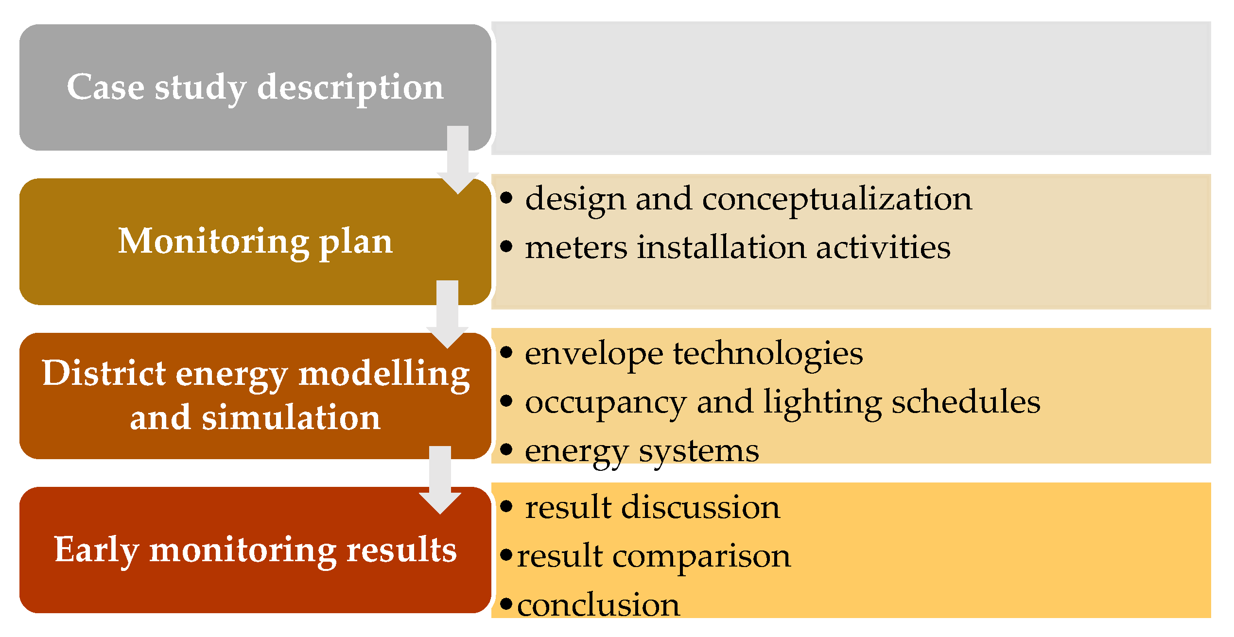
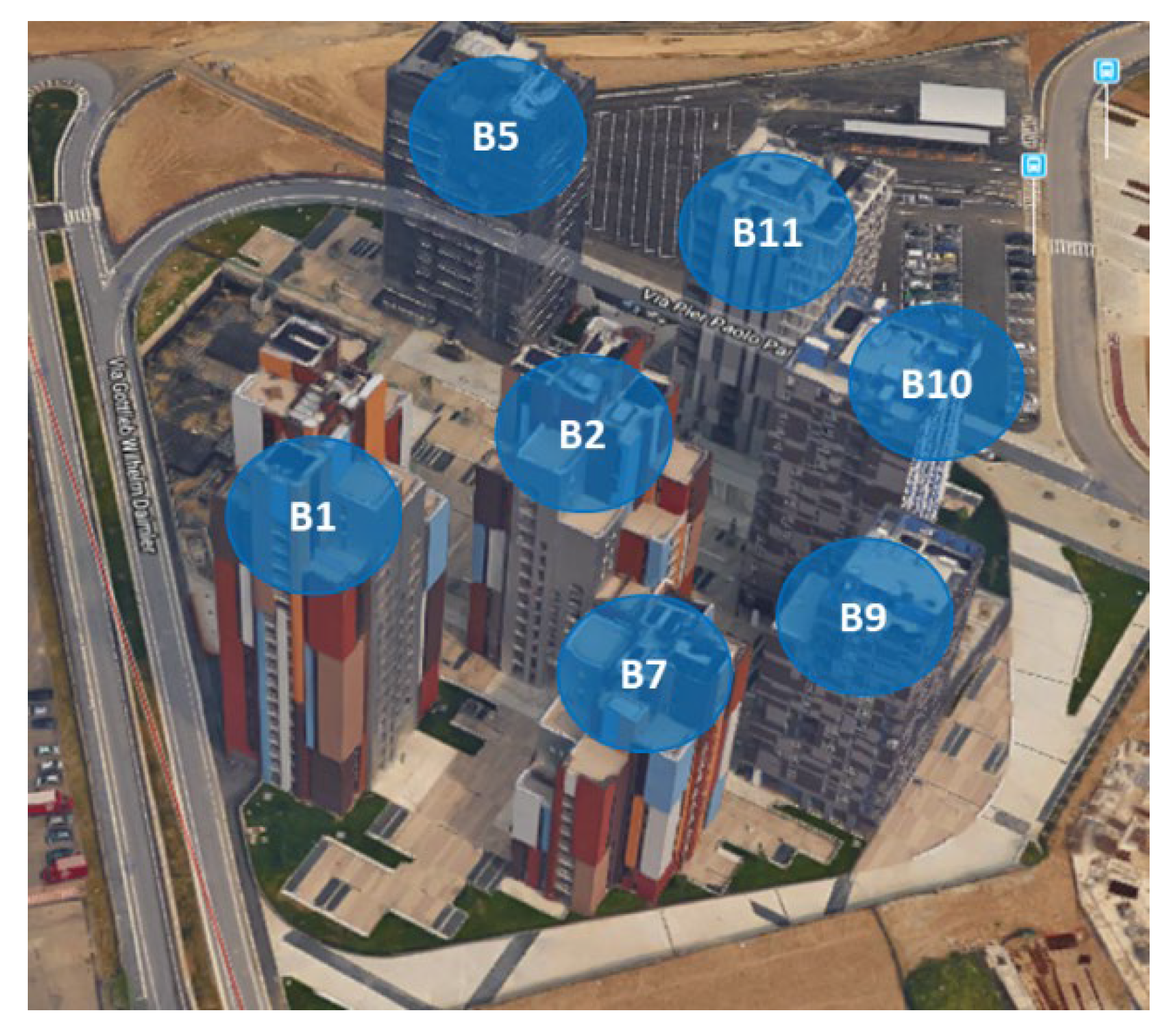
2. The Case Study
3. Monitoring Plan
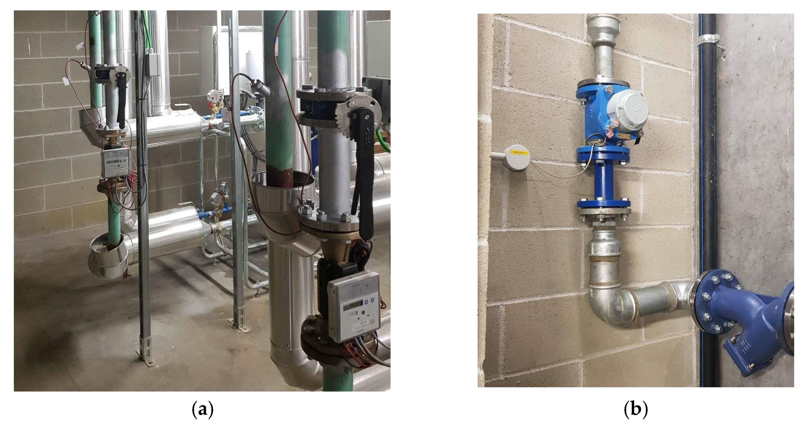
3.1. New Meters Installation and Data Acquisition System
3.1.1. Cooling System
3.1.2. Heating and DHW Systems
3.1.3. Buildings Distribution Circuits
3.1.4. Controlled Mechanical Ventilation (CMV)
3.1.5. Photovoltaic System
3.1.6. Lighting and Appliances
3.1.7. Single Apartment Mechanical Systems and Indoor Comfort Conditions
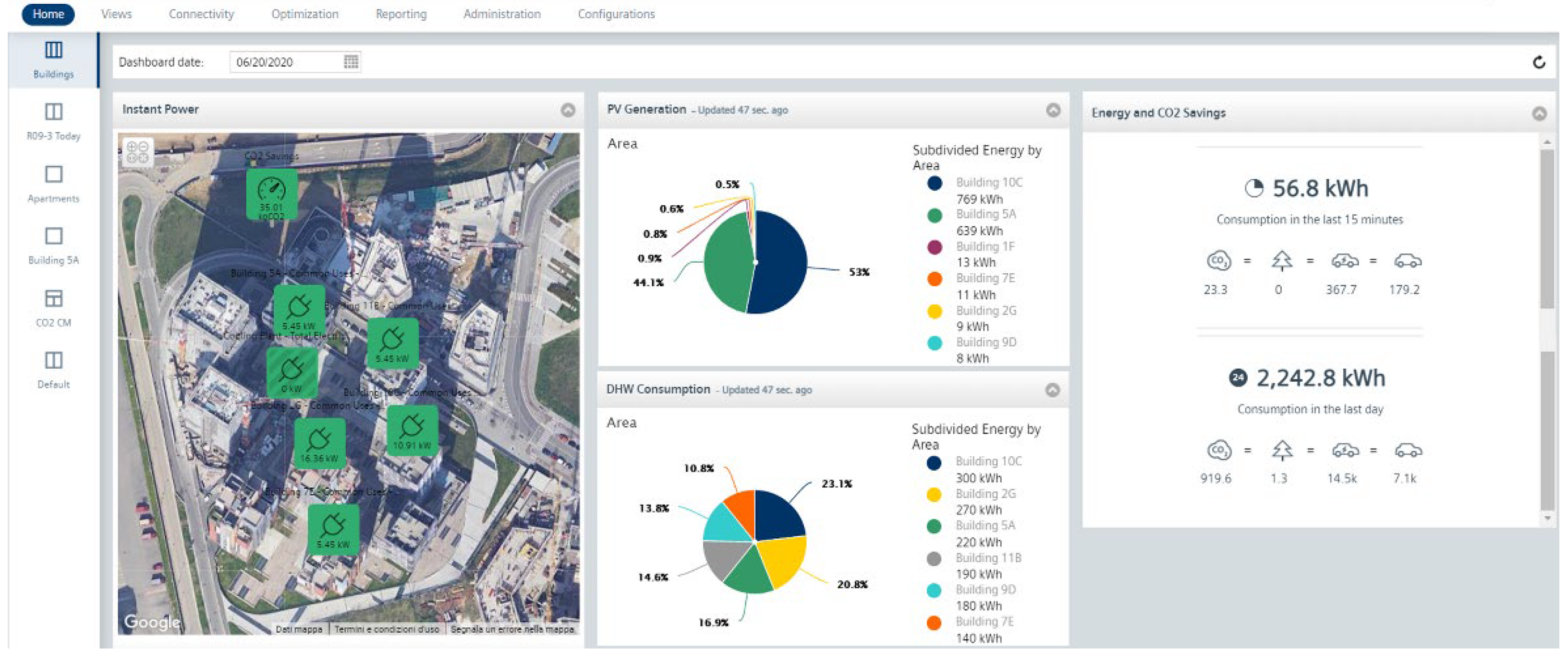
3.2. Energy Management System
4. Modeling
4.1. Buildings’ Modeling
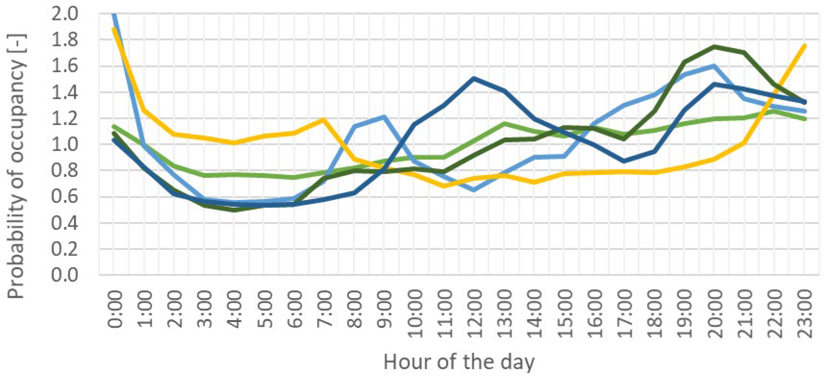
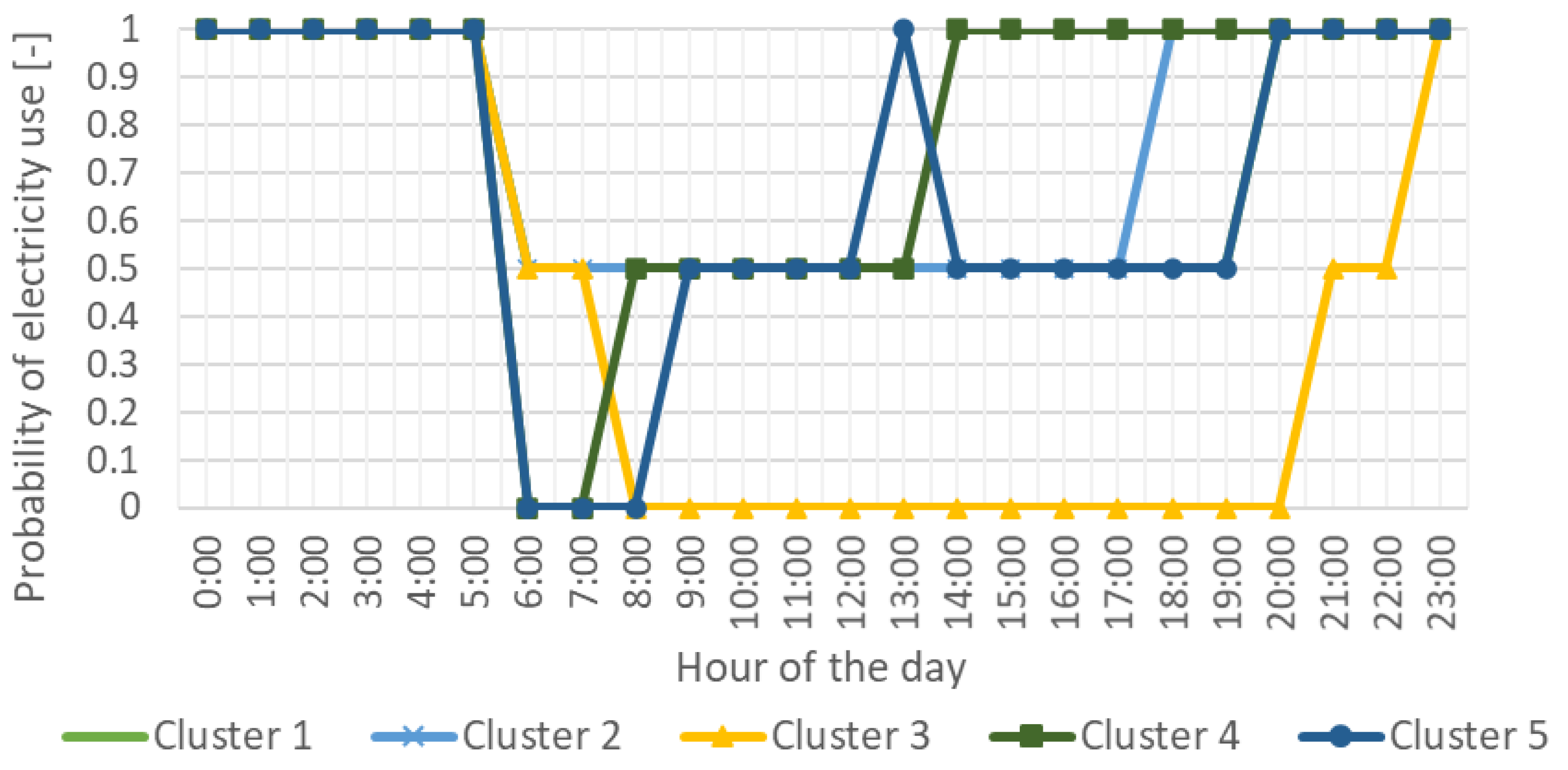
Occupant Behavior
4.2. HVAC System Modeling
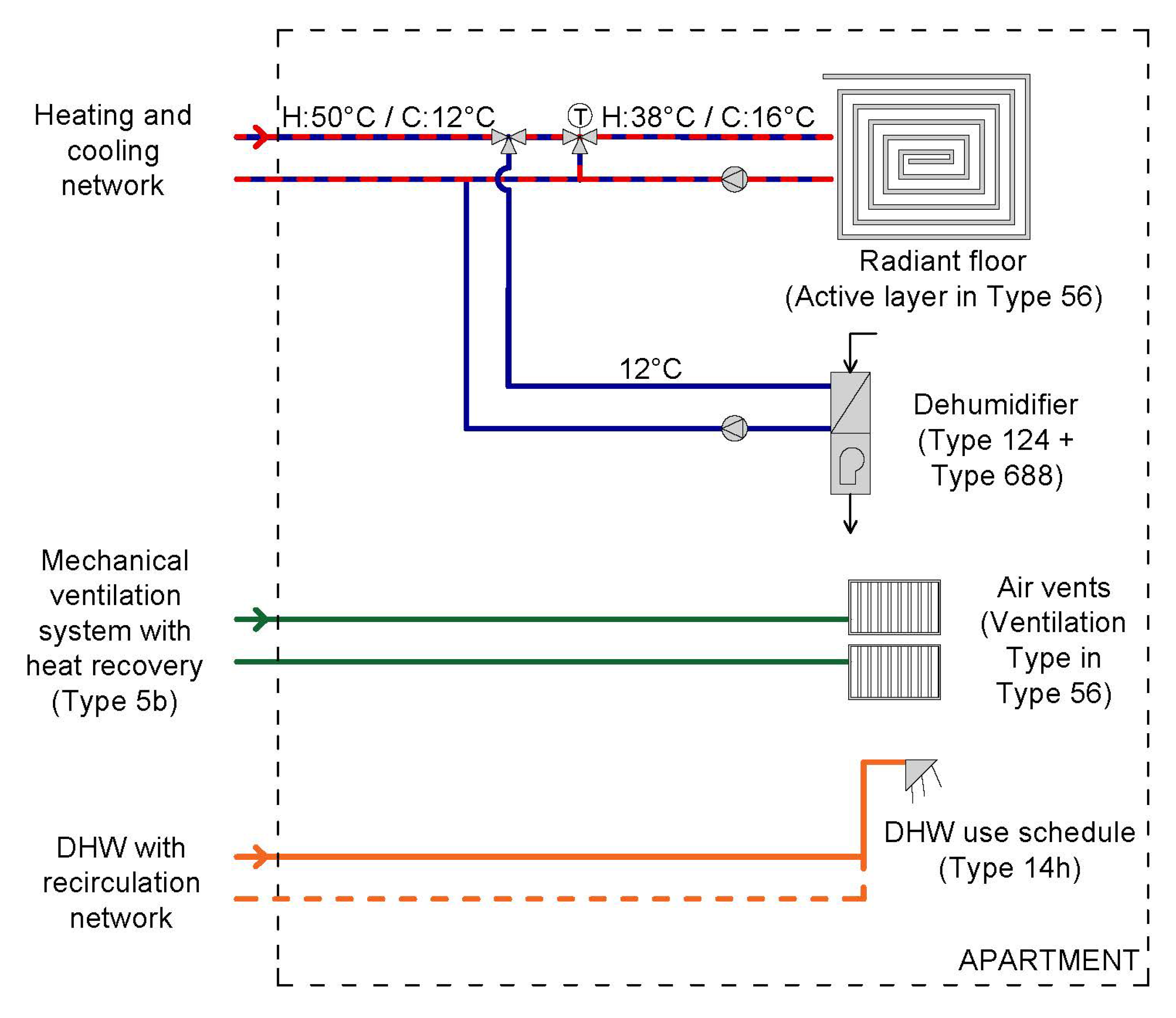
4.2.1. Apartment System Layout
- Radiant floor panels
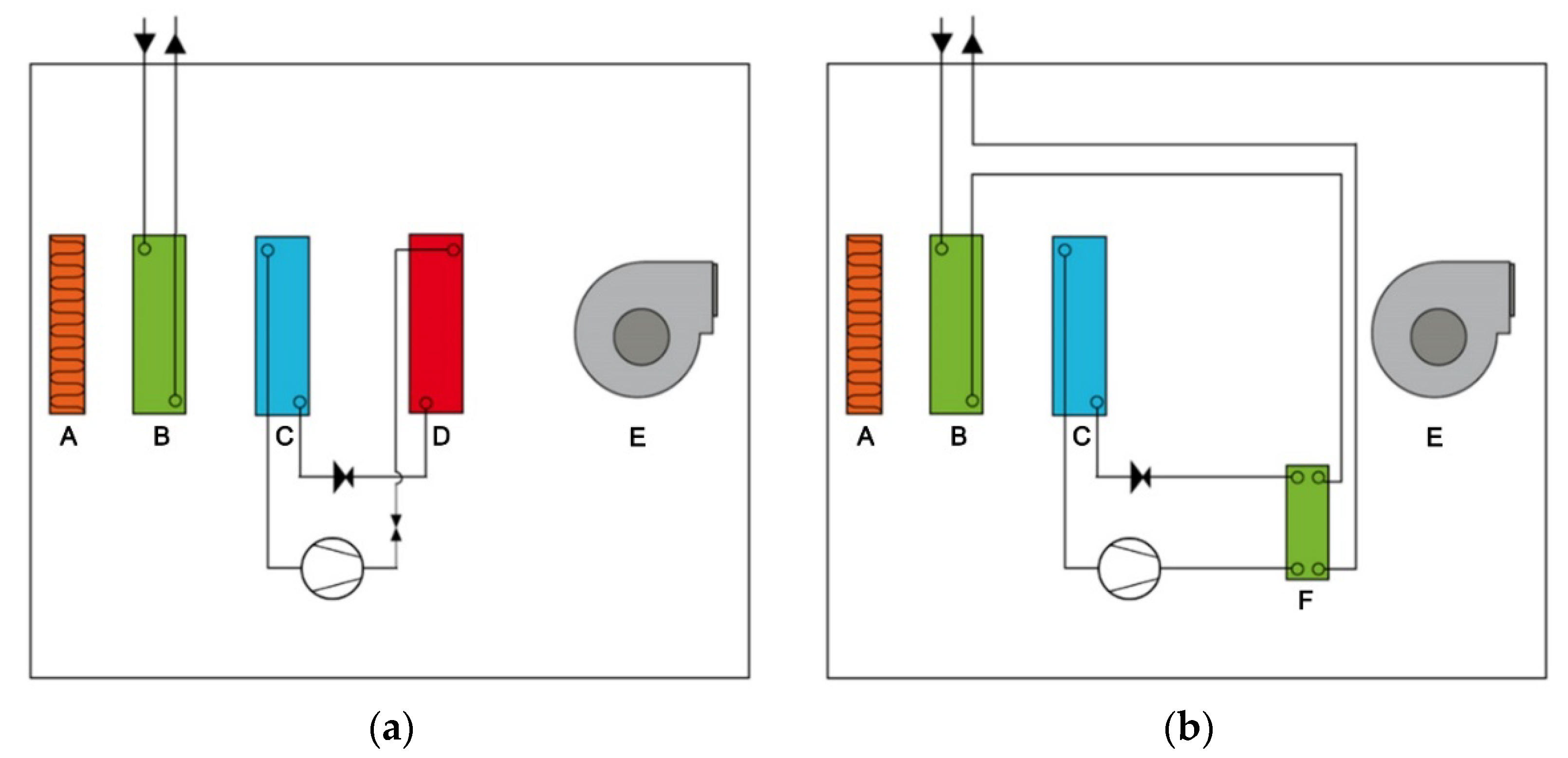
- Dehumidifier
- Mechanical ventilation system
- Domestic hot water production
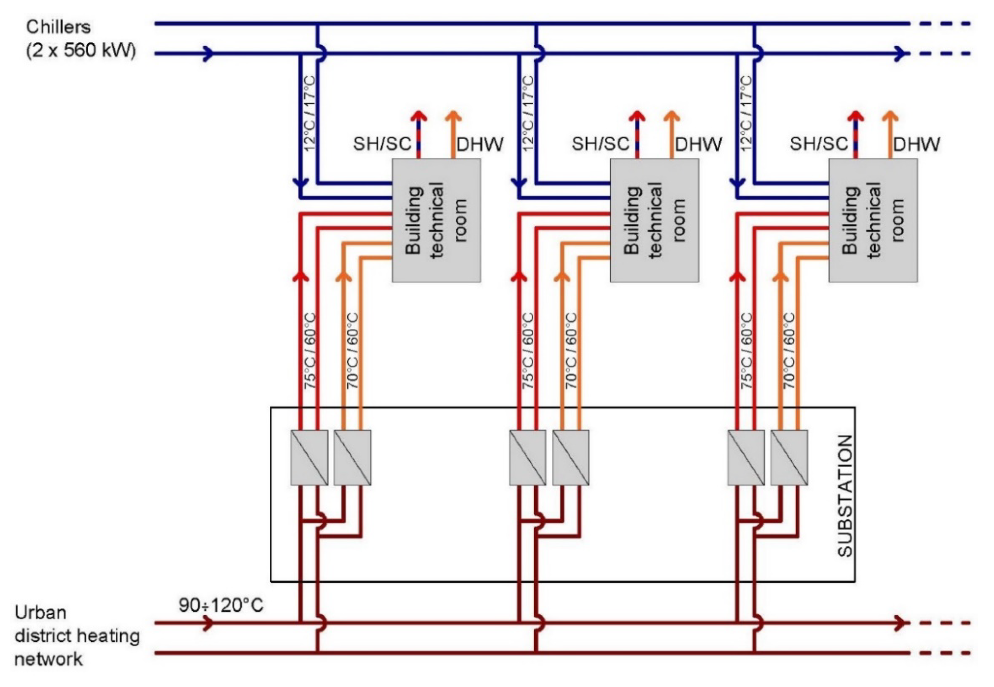
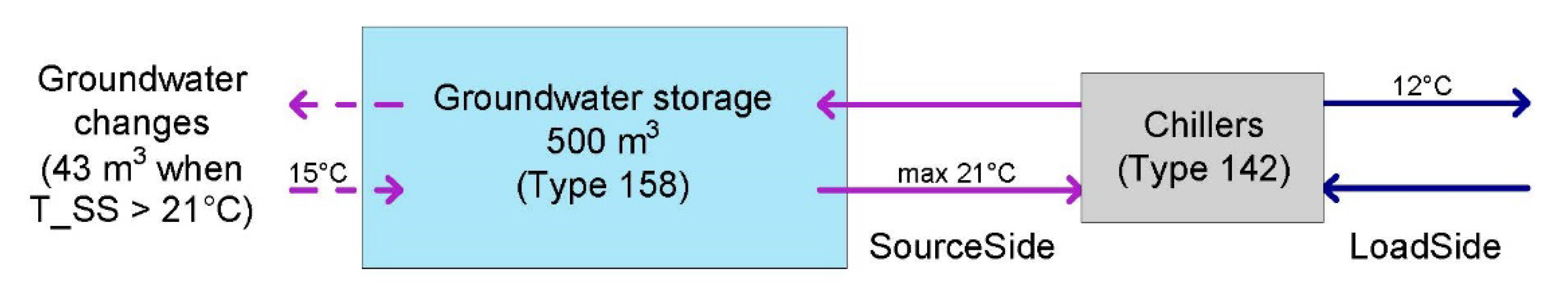
4.2.2. District Systems Layout
5. Results and Discussion
5.1. Simulation Results
5.2. Early Monitoring Results
6. Conclusions
- Complex neighborhood/district energy networks should always be built together with an EMS to provide remote control. System faults are highly probable, and optimization is needed from the first operational day;
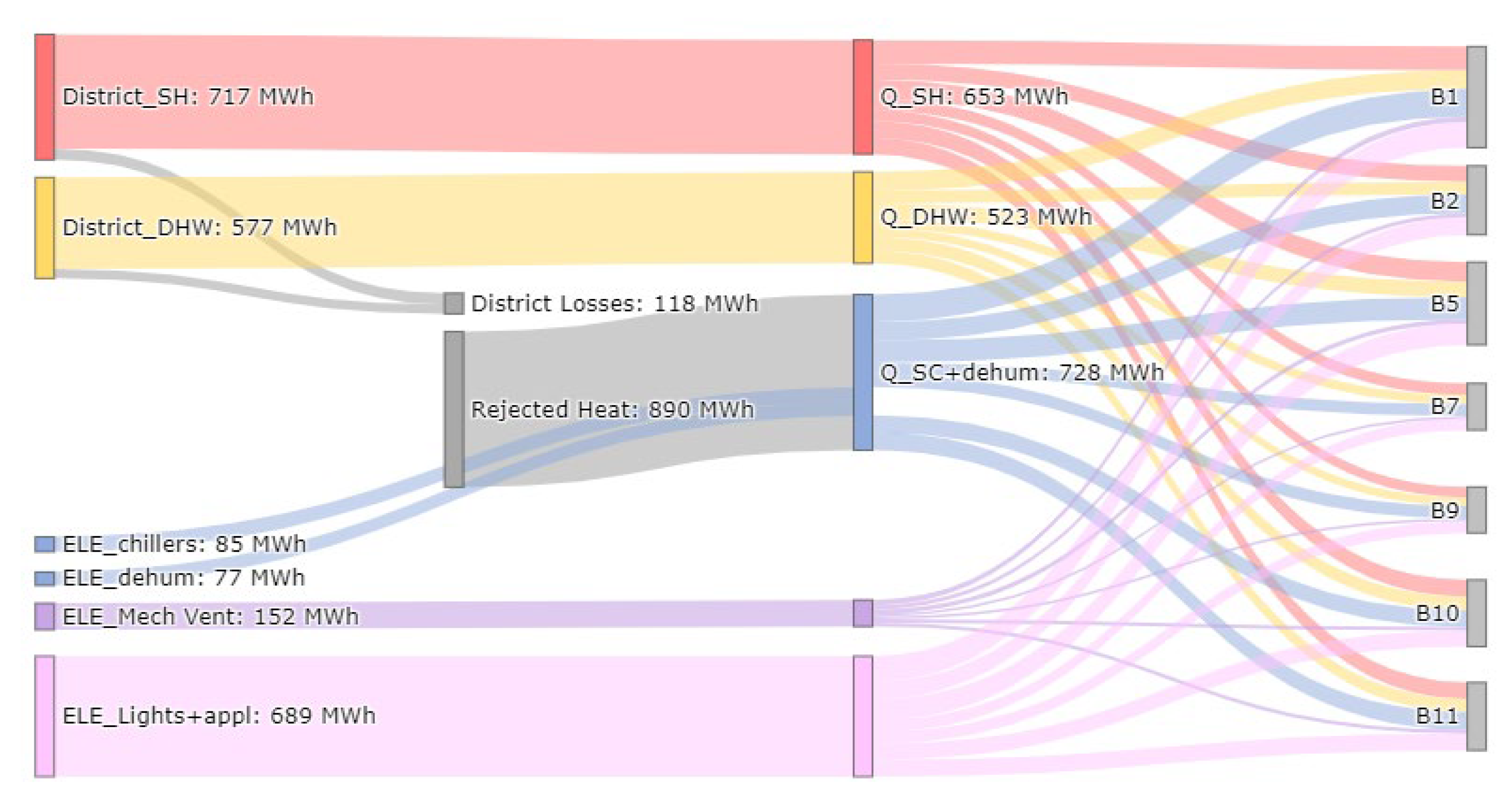
- Space heating and DHW production are relevant uses (respectively 34% and 28% of the thermal energy needs), and geothermal energy might be used to cover them with higher efficiencies;
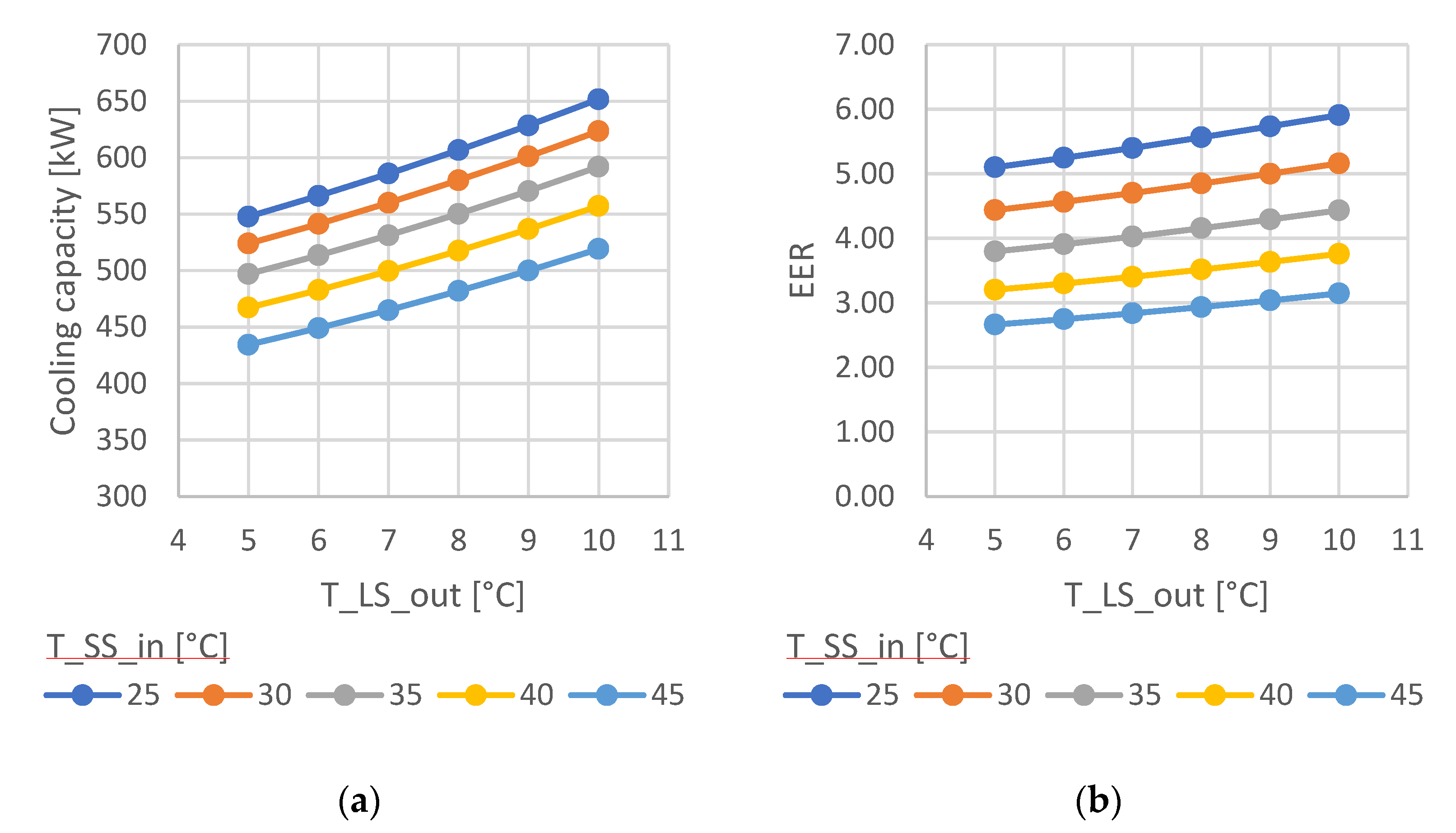
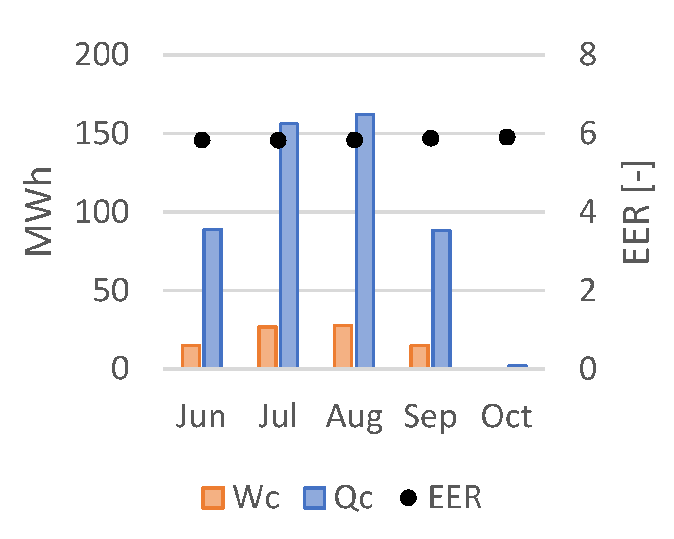
- The use of centralized water-source cooling systems should be promoted under the specific boundary conditions, due to the high efficiency (EER equal to 5.84) compared to individual air-source systems;
- Lights and appliances are a large share of the electricity use (about 70% of total electrical consumptions), a higher occupant engagement should, thus, be promoted;
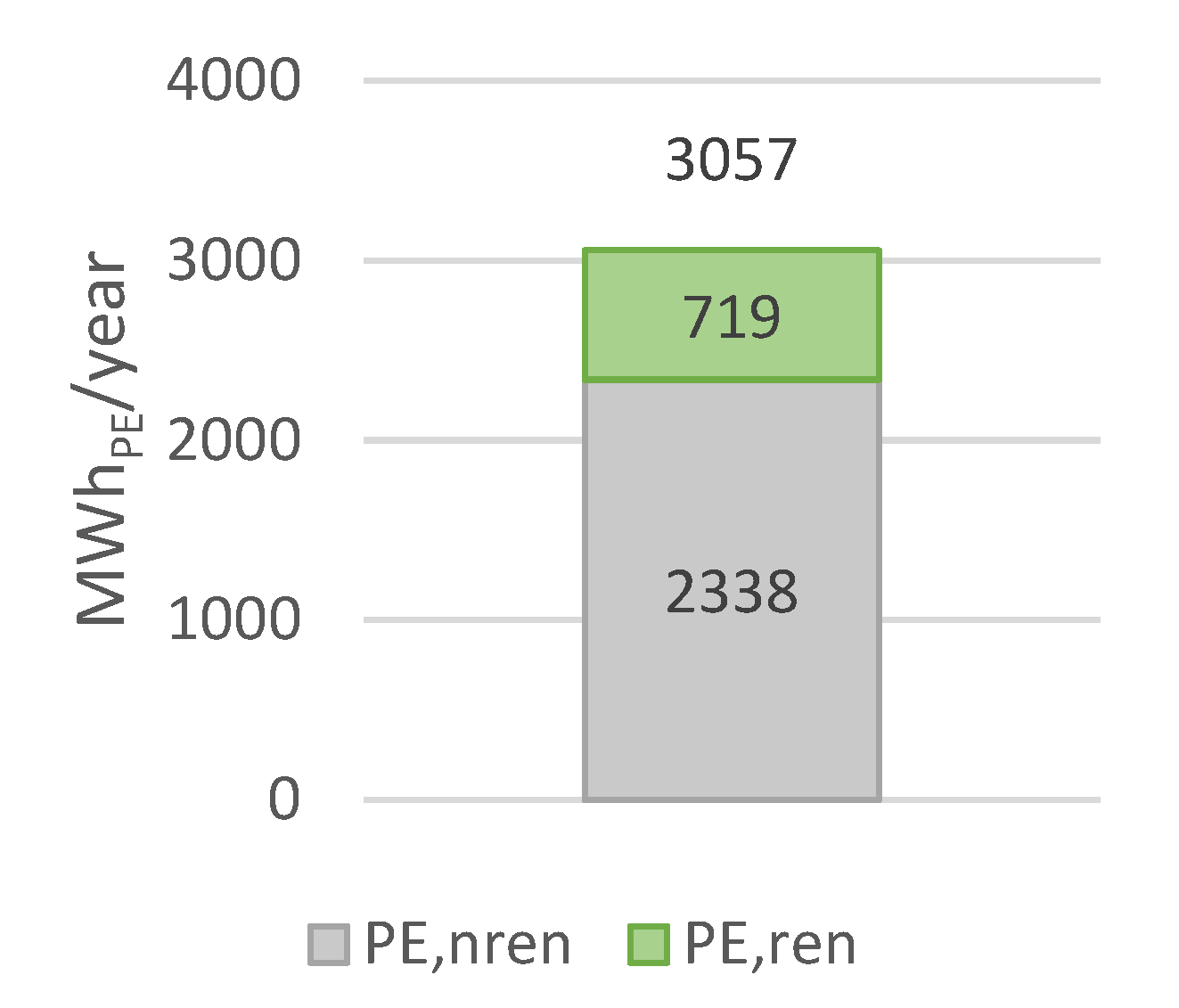
- In order to reach a level of decarbonization in line with the Municipality’s targets, the neighborhood needs to substantially increase its share of renewable energy.
Supplementary Materials
Author Contributions
Funding
Acknowledgments
Conflicts of Interest
References
- UN-Habitat Energy. UN-Habitat. Available online: https://new.unhabitat.org/topic/energy (accessed on 26 March 2021).
- Causone, F.; Sangalli, A.; Pagliano, L.; Carlucci, S. Assessing energy performance of smart cities. Build. Serv. Eng. Res. Technol. 2018, 39, 99–116. [Google Scholar] [CrossRef] [Green Version]
- IEA European Union 2020—Analysis—IEA. Available online: https://www.iea.org/reports/european-union-2020 (accessed on 26 March 2021).
- European Commission Energy Performance of Buildings Directive. Energy. Available online: https://ec.europa.eu/energy/topics/energy-efficiency/energy-efficient-buildings/energy-performance-buildings-directive_en?redir=1 (accessed on 26 March 2021).
- European Commission. New Rules for Greener and Smarter Buildings will Increase Quality of Life for All Europeans. Available online: https://ec.europa.eu/info/news/new-rules-greener-and-smarter-buildings-will-increase-quality-life-all-europeans-2019-apr-15_en (accessed on 26 March 2021).
- Park, K.; Kim, Y.; Kim, S.; Kim, K.; Lee, W.; Park, H. Building Energy Management System based on Smart Grid. In Proceedings of the 2011 IEEE 33rd International Telecommunications Energy Conference (INTELEC), Amsterdam, The Netherlands, 9–13 October 2011; pp. 1–4. [Google Scholar]
- Zucker, G.; Judex, F.; Blöchle, M.; Köstl, M.; Widl, E.; Hauer, S.; Bres, A.; Zeilinger, J. A new method for optimizing operation of large neighborhoods of buildings using thermal simulation. Energy Build. 2016, 125, 153–160. [Google Scholar] [CrossRef]
- Aprile, M.; Scoccia, R.; Dénarié, A.; Kiss, P.; Dombrovszky, M.; Gwerder, D.; Schuetz, P.; Elguezabal, P.; Arregi, B. District power-to-heat/cool complemented by sewage heat recovery. Energies 2019, 12, 364. [Google Scholar] [CrossRef] [Green Version]
- Dénarié, A.; Muscherà, M.; Calderoni, M.; Motta, M. Industrial excess heat recovery in district heating: Data assessment methodology and application to a real case study in Milano, Italy. Energy 2019, 166, 170–182. [Google Scholar] [CrossRef]
- King, J.C. Perry Smart Buildings: Using Smart Technology to Save Energy in Existing Buildings. Am. Counc. Energy-Efficient Econ. 2017, 1–46. [Google Scholar]
- Wurtz, F.; Delinchant, B. “Smart buildings” integrated in “smart grids”: A key challenge for the energy transition by using physical models and optimization with a “human-in-the-loop” approach. Comptes Rendus Phys. 2017, 18, 428–444. [Google Scholar] [CrossRef]
- Kim, H.; Choi, H.; Kang, H.; An, J.; Yeom, S.; Hong, T. A systematic review of the smart energy conservation system: From smart homes to sustainable smart cities. Renew. Sustain. Energy Rev. 2021, 140, 110755. [Google Scholar] [CrossRef]
- Causone, F.; Tatti, A.; Pietrobon, M.; Zanghirella, F.; Pagliano, L. Yearly operational performance of a nZEB in the Mediterranean climate. Energy Build. 2019, 198, 243–260. [Google Scholar] [CrossRef] [Green Version]
- Anda, M.; Temmen, J. Smart metering for residential energy efficiency: The use of community based social marketing for behavioural change and smart grid introduction. Renew. Energy 2014, 67, 119–127. [Google Scholar] [CrossRef]
- Paetz, A.G.; Dütschke, E.; Fichtner, W. Smart Homes as a Means to Sustainable Energy Consumption: A Study of Consumer Perceptions. J. Consum. Policy 2012, 35, 23–41. [Google Scholar] [CrossRef]
- Sirombo, E.; Filippi, M.; Catalano, A.; Sica, A. Building monitoring system in a large social housing intervention in Northern Italy. Energy Procedia 2017, 140, 386–397. [Google Scholar] [CrossRef]
- Lobaccaro, G.; Carlucci, S.; Löfström, E. A Review of Systems and Technologies for Smart Homes and Smart Grids. Energies 2016, 9, 348. [Google Scholar] [CrossRef] [Green Version]
- Shakeri, M.; Pasupuleti, J.; Amin, N.; Rokonuzzaman, M.; Low, F.W.; Yaw, C.T.; Asim, N.; Samsudin, N.A.; Tiong, S.K.; Hen, C.K.; et al. An Overview of the Building Energy Management System Considering the Demand Response Programs, Smart Strategies and Smart Grid. Energies 2020, 13, 3299. [Google Scholar] [CrossRef]
- Fonseca, J.A.; Nguyen, T.-A.; Schlueter, A.; Marechal, F. City Energy Analyst (CEA): Integrated framework for analysis and optimization of building energy systems in neighborhoods and city districts. Energy Build. 2016, 113, 202–226. [Google Scholar] [CrossRef]
- Hu, M.; Xiao, F.; Wang, S. Neighborhood-level coordination and negotiation techniques for managing demand-side flexibility in residential microgrids. Renew. Sustain. Energy Rev. 2021, 135, 110248. [Google Scholar] [CrossRef]
- Ferrando, M.; Causone, F. An Overview Of Urban Building Energy Modelling (UBEM) Tools. In Proceedings of the Building Simulation 2019: 16th Conference of IBPSA, Rome, Italy, 2–4 September 2020; Volume 16, pp. 3452–3459. [Google Scholar]
- Ferrando, M.; Causone, F.; Hong, T.; Chen, Y. Urban building energy modeling (UBEM) tools: A state-of-the-art review of bottom-up physics-based approaches. Sustain. Cities Soc. 2020, 62, 102408. [Google Scholar] [CrossRef]
- Causone, F.; Pelle, M. Building stock simulation to support the development of a district multi-energy grid. E3S Web Conf. 2019, 111, 6027. [Google Scholar] [CrossRef]
- Carnieletto, L.; Ferrando, M.; Teso, L.; Sun, K.; Zhang, W.; Causone, F.; Romagnoni, P.; Zarrella, A.; Hong, T. Italian prototype building models for urban scale building performance simulation. Build. Environ. 2021, 192, 107590. [Google Scholar] [CrossRef]
- Tuballa, M.L.; Abundo, M.L. A review of the development of Smart Grid technologies. Renew. Sustain. Energy Rev. 2016, 59, 710–725. [Google Scholar] [CrossRef]
- Ajaz, W.; Bernell, D. California’s adoption of microgrids: A tale of symbiotic regimes and energy transitions. Renew. Sustain. Energy Rev. 2021, 138, 110568. [Google Scholar] [CrossRef]
- Mostafa, M.H.; Abdel Aleem, S.H.E.; Ali, S.G.; Abdelaziz, A.Y. Energy-management solutions for microgrids. In Distributed Energy Resources in Microgrids: Integration, Challenges and Optimization; Elsevier: Amsterdam, The Netherlands, 2019; pp. 483–515. ISBN 9780128177747. [Google Scholar]
- European University Association. Energy Transition and the Future of Energy Research, Innovation and Education: An Action Agenda for European Universities. Int. J. Prod. Res. 2017, 53, 59. [Google Scholar]
- Conci, M.; Schneider, J. A District Approach to Building Renovation for the Integral Energy Redevelopment of Existing Residential Areas. Sustainability 2017, 9, 747. [Google Scholar] [CrossRef] [Green Version]
- Ipakchi, A.; Albuyeh, F. Grid of the future. IEEE Power Energy Mag. 2009, 7, 52–62. [Google Scholar] [CrossRef]
- Mattoni, B.; Nardecchia, F.; Bisegna, F. Towards the development of a smart district: The application of an holistic planning approach. Sustain. Cities Soc. 2019, 48, 101570. [Google Scholar] [CrossRef]
- Allegrini, J.; Orehounig, K.; Mavromatidis, G.; Ruesch, F.; Dorer, V.; Evins, R. A review of modelling approaches and tools for the simulation of district-scale energy systems. Renew. Sustain. Energy Rev. 2015, 52, 1391–1404. [Google Scholar] [CrossRef]
- Schweiger, G.; Heimrath, R.; Falay, B.; O’Donovan, K.; Nageler, P.; Pertschy, R.; Engel, G.; Streicher, W.; Leusbrock, I. District energy systems: Modelling paradigms and general-purpose tools. Energy 2018, 164, 1326–1340. [Google Scholar] [CrossRef]
- Salvia, G.; Morello, E.; Rotondo, F.; Sangalli, A.; Causone, F.; Erba, S.; Pagliano, L. Performance gap and occupant behavior in building retrofit: Focus on dynamics of change and continuity in the practice of indoor heating. Sustainability 2020, 12, 5820. [Google Scholar] [CrossRef]
- Kampelis, N.; Papayiannis, G.I.; Kolokotsa, D.; Galanis, G.N.; Isidori, D.; Cristalli, C.; Yannacopoulos, A.N. An integrated energy simulation model for buildings. Energies 2020, 13, 1170. [Google Scholar] [CrossRef] [Green Version]
- Angelotti, A.; Ballabio, M.; Mazzarella, L.; Cornaro, C.; Parente, G.; Frasca, F.; Prada, A.; Baggio, P.; Ballarini, I.; De Luca, G.; et al. Dynamic Simulation of existing buildings: Considerations on the Model Calibration. In Proceedings of the Building Simulation 2019: 16th Conference of IBPSA, Rome, Italy, 2–4 September 2020; Volume 16, pp. 4165–4172. [Google Scholar]
- Fabrizio, E.; Monetti, V. Methodologies and Advancements in the Calibration of Building Energy Models. Energies 2015, 8, 2548–2574. [Google Scholar] [CrossRef] [Green Version]
- The Solar Energy Laboratory—University of Wisconsin-Madison TRNSYS 18—A TRaNsient SYstem Simulation program. Available online: https://sel.me.wisc.edu/trnsys/ (accessed on 31 March 2021).
- Causone, F.; Sangalli, A.; Pagliano, L.; Carlucci, S. An Exergy Analysis for Milano Smart City. Energy Procedia 2017, 111, 867–876. [Google Scholar] [CrossRef] [Green Version]
- Lund, H.; Østergaard, P.A.; Connolly, D.; Mathiesen, B.V. Smart energy and smart energy systems. Energy 2017, 137, 556–565. [Google Scholar] [CrossRef]
- Caputo, P.; Costa, G.; Ferrari, S. A supporting method for defining energy strategies in the building sector at urban scale. Energy Policy 2013, 55, 261–270. [Google Scholar] [CrossRef]
- Guerra Santin, O.; Itard, L.; Visscher, H. The effect of occupancy and building characteristics on energy use for space and water heating in Dutch residential stock. Energy Build. 2009, 41, 1223–1232. [Google Scholar] [CrossRef]
- Causone, F.; Carlucci, S.; Ferrando, M.; Marchenko, A.; Erba, S. A data-driven procedure to model occupancy and occupant-related electric load profiles in residential buildings for energy simulation. Energy Build. 2019, 202, 109342. [Google Scholar] [CrossRef]
- A2A Calore e Servizi S.r.l. Certificazione Energetica in Presenza di Teleriscaldamento (Milano Ovest). 2018. Available online: http://www.a2acaloreservizi.eu/home/cms/a2a_caloreservizi/impianti_reti/area_milano/.
- Regione Lombardia. DDUO 2456/2017; Associazione Nazionale per l’Isolamento Termico e Acustico: Milano, Italy, 2017. [Google Scholar]
- International Organisation for Standardisation. EN ISO 52000-1:2017 Energy Performance of Buildings—Overarching EPB Assessment Part1: General Framework and Procedures; International Organisation for Standardisation: Geneva, Switzerland, 2017. [Google Scholar]
- Weather Data by Location. EnergyPlus. Available online: https://energyplus.net/weather-location/europe_wmo_region_6/ITA//ITA_Milano-Linate.160800_IGDG (accessed on 31 March 2021).


| One Room | Two Rooms | Three Rooms | Four Rooms | Five Rooms | Tot | |
|---|---|---|---|---|---|---|
| B1 | 0 | 16 | 49 | 17 | 1 | 83 |
| B2 | 0 | 13 | 31 | 12 | 1 | 57 |
| B5 | 0 | 14 | 45 | 10 | 0 | 69 |
| B7 | 1 | 3 | 35 | 0 | 0 | 38 |
| B9 | 0 | 10 | 18 | 10 | 0 | 38 |
| B10 | 0 | 1 | 54 | 0 | 0 | 55 |
| B11 | 0 | 7 | 42 | 7 | 0 | 56 |
| Tot | 1 | 64 | 274 | 56 | 2 | 396 |
| Construction Scale | Monitoring Target | Indicator | Meter | Number of Meters | Measured Parameters | Unit of Measure | Number of Measured Parameters | Data Owner | Sensor Accuracy | Sensor Resolution | Frequency of Data Acquisition | Frequency of Data Recording | Frequency of Data Transmission | Data Transmission Protocol | ||
|---|---|---|---|---|---|---|---|---|---|---|---|---|---|---|---|---|
| Building | Parcel | District | Heating system | |||||||||||||
| DHW | ||||||||||||||||
| Cooling system | ||||||||||||||||
| CMV | ||||||||||||||||
| Lighting and appliances | ||||||||||||||||
| PV system | ||||||||||||||||
| Apartment indoor Comfort conditions | ||||||||||||||||
| Vgross [m3] | Vnet [m3] | SEXT,gross [m2] | Suseful [m2] | S/V [-] | WWR [m2] | N° of Floors | |
|---|---|---|---|---|---|---|---|
| B1 | 23,281 | 16,533 | 6361 | 6123 | 27% | 19% | 23 |
| B2 | 16,552 | 11,088 | 6594 | 4106 | 40% | 13% | 18 |
| B5 | 19,194 | 12,524 | 6832 | 4638 | 36% | 15% | 17 |
| B7 | 11,350 | 7572 | 5536 | 2805 | 49% | 11% | 11 |
| B9 | 10,564 | 7096 | 4596 | 2628 | 44% | 11% | 14 |
| B10 | 17,246 | 12,875 | 7700 | 4768 | 45% | 13% | 17 |
| B11 | 13,118 | 8995 | 5223 | 3331 | 40% | 22% | 17 |
| ID | B1 | B2–B7 | B9–B10 | B11 | B5 |
|---|---|---|---|---|---|
| M1 | 0.175 | 0.161 | 0.161 | 0.161 | 0.161 |
| M2 | 0.219 | 0.219 | 0.219 | 0.219 | 0.219 |
| M5 | 0.236 | 0.236 | 0.236 | 0.236 | 0.236 |
| M6 | 0.341 | 0.341 | 0.341 | 0.341 | 0.341 |
| P1 | 0.490 | 0.490 | 0.490 | 0.490 | 0.490 |
| P2 | 0.266 | 0.266 | 0.147 | 0.287 | 0.136 |
| S4 | 0.204 | 0.204 | 0.180 | 0.180 | 0.180 |
| Apartment Typology | Wh | People |
|---|---|---|
| Two room | 165.5 | 2 |
| Three room | 198.1 | 3 |
| Four room | 202.5 | 5 |
| Zone Type | Water Flow Rate (L/h) | Number of Loops |
| 1 | 536.8 | 9 |
| 2 | 500.2 | 9 |
| 3 | 577.8 | 9 |
| 4 | 395.4 | 6 |
| 5 | 787.2 | 12 |
Publisher’s Note: MDPI stays neutral with regard to jurisdictional claims in published maps and institutional affiliations. |
© 2021 by the authors. Licensee MDPI, Basel, Switzerland. This article is an open access article distributed under the terms and conditions of the Creative Commons Attribution (CC BY) license (https://creativecommons.org/licenses/by/4.0/).
Share and Cite
Causone, F.; Scoccia, R.; Pelle, M.; Colombo, P.; Motta, M.; Ferroni, S. Neighborhood Energy Modeling and Monitoring: A Case Study. Energies 2021, 14, 3716. https://doi.org/10.3390/en14123716
Causone F, Scoccia R, Pelle M, Colombo P, Motta M, Ferroni S. Neighborhood Energy Modeling and Monitoring: A Case Study. Energies. 2021; 14(12):3716. https://doi.org/10.3390/en14123716
Chicago/Turabian StyleCausone, Francesco, Rossano Scoccia, Martina Pelle, Paola Colombo, Mario Motta, and Sibilla Ferroni. 2021. "Neighborhood Energy Modeling and Monitoring: A Case Study" Energies 14, no. 12: 3716. https://doi.org/10.3390/en14123716
APA StyleCausone, F., Scoccia, R., Pelle, M., Colombo, P., Motta, M., & Ferroni, S. (2021). Neighborhood Energy Modeling and Monitoring: A Case Study. Energies, 14(12), 3716. https://doi.org/10.3390/en14123716