Article

Gate Road Support Deformation Forecasting Based on Multivariate Singular Spectrum Analysis and Fuzzy Time Series

Faculty of Mining and Geology, University of Belgrade, Đušina 7, 11000 Belgrade, Serbia
*
Author to whom correspondence should be addressed.
Energies 2021, 14(12), 3710; https://doi.org/10.3390/en14123710
Submission received: 19 May 2021 / Revised: 10 June 2021 / Accepted: 14 June 2021 / Published: 21 June 2021
(This article belongs to the Special Issue Mining Innovation)

Abstract

:
Underground mining engineers and planners in our country are faced with extremely difficult working conditions and a continuous shortage of money. Production disruptions are frequent and can sometimes last more than a week. During this time, gate road support is additionally exposed to rock stress and the result is its progressive deformation and the loss of functionality of gate roads. In such an environment, it is necessary to develop a low-cost methodology to maintain a gate road support system. For this purpose, we have developed a model consisting of two main phases. The first phase is related to support deformation monitoring, while the second phase is related to data analysis. To record support deformations over a defined time horizon we use laser scanning technology together with multivariate singular spectrum analysis to conduct data processing and forecasting. Fuzzy time series is applied to classify the intensity of displacements into several independent groups (clusters).

1. Introduction

Due to hard working conditions and a chronic shortage of money, the underground mining in our country is very a difficult task. Most underground mines are characterized by low mechanized mining methods and production disruptions can happen often. Such mining methods are characterized by a long production cycle, and if we add disruptions then it is obvious that the gate road support is exposed to the rock stress much longer than is the case with the application of modern mechanized methods. In such a production environment, the maintenance of the gate road stability is almost impossible and is performed in an unsystematic way. In order to improve such a difficult situation, we use a laser scanner to obtain high accuracy deformation data, and multivariate singular spectrum analysis to process them and forecast the future state of deformations. Fuzzy time series is used to classify deformation data into several independent groups with respect to the magnitude of deformation intensity. In this way, we are enabling underground mining engineers to develop a plan to support maintenance. They can plan activities related to the identification of support states in the future, time of reconstruction, and type of support that can be used to decrease the progressive deformation. An effective deformation forecast can result in a decrease of costs and delays.
There are many different approaches to obtaining future states of support deformation. Ding-Ping Xu et al. [1] compared the predictions from the rock–soil composite material model, where an analytic method, along with existing data from physical model tests, was applied to acquire results. Good consistency, both in terms of strength and failure mode, was provided when a comparison of these three types of information was done [1]. Danial Jahed Armaghani et al. [2] applied three-nonlinear forecasting methods, namely a non-linear multiple regression, an artificial neural network, and an adaptive neuro-fuzzy inference system, in order to estimate the uniaxial compressive strength of rock.
Grey system prediction models were developed by Xiaobo Xiong [3] for forecasting rock tunnel displacement considering the non-linear parameters of the deformation of the tunnel. Ping Tang [4] forecasted the working face underground pressure by applying a grey system theory and genetic algorithm. Sun Yu et al. [5] proposed a time series prediction model based on a generalized regression neural network to predict the long-term potential deformation trends of surrounding rocks in a soft rock roadway tunnel. Haiming Chen et al. [6] built an intelligent displacement back analysis network of a deep mine roadway surrounding rock that is based on MATLAB NN toolbox. Francesca Bozzano et al. [7] used terrestrial SAR interferometry to support the management of each phase of tunneling. Qian Zhang et al. [8] made a numerical simulation for advanced displacement of tunnel with weak and broken surrounding rock in order to reveal the adjusting process of displacement in the main parts of a tunnel.
Grossauer et al. [9] developed an efficient way to predict displacements caused by tunnel excavation based on the use of analytical functions that describe the movements as a function of time and the face advance. A procedure based on analytical functions has been developed to support the prediction of the tunnel performance and surface movements. Merlini and Falanesca [10] illustrated the comparison between the prognosis and the crosscheck of the support methods and the replacement solutions. Several back- analyses were carried out in order to achieve the correct validation of the interventions and an optimal understanding of the deformation behavior of the rock mass. Bao-Zhen Yao et al. [11] has presented a multi-step-ahead prediction model, based on a support vector machine, for tunnel surrounding rock displacement forecasting.
This paper is divided into five sections. In the section Materials and Methods, we describe the model of forecasting based on observed data and multivariate singular spectrum analysis. We introduce the fuzzy time series concept to make clusters describing the gate road support configuration deformation for every time point over observed and forecasted periods. A computational process is performed in the Numerical Example section to represent the possibilities of model and conclusions are provided in the Results and Conclusion section. Obtained results show a high level of correlation of original and reconstructed series of the support deformations. Based on these results, it can be concluded that the model is reliable and applicable for solving real-time problems in terms of predicting gate road support deformations.

2. Materials and Methods

2.1. Dynamic of Support Deformations

The dynamic behavior of support is induced by the rock stress surrounding the gate road. Deformation dynamics is the study of time varying response of support under dynamic loads. These loads are primarily considered a change of rock stress intensity induced by mining activities. As a stope approaches the gate road, the rock stress intensity increases.
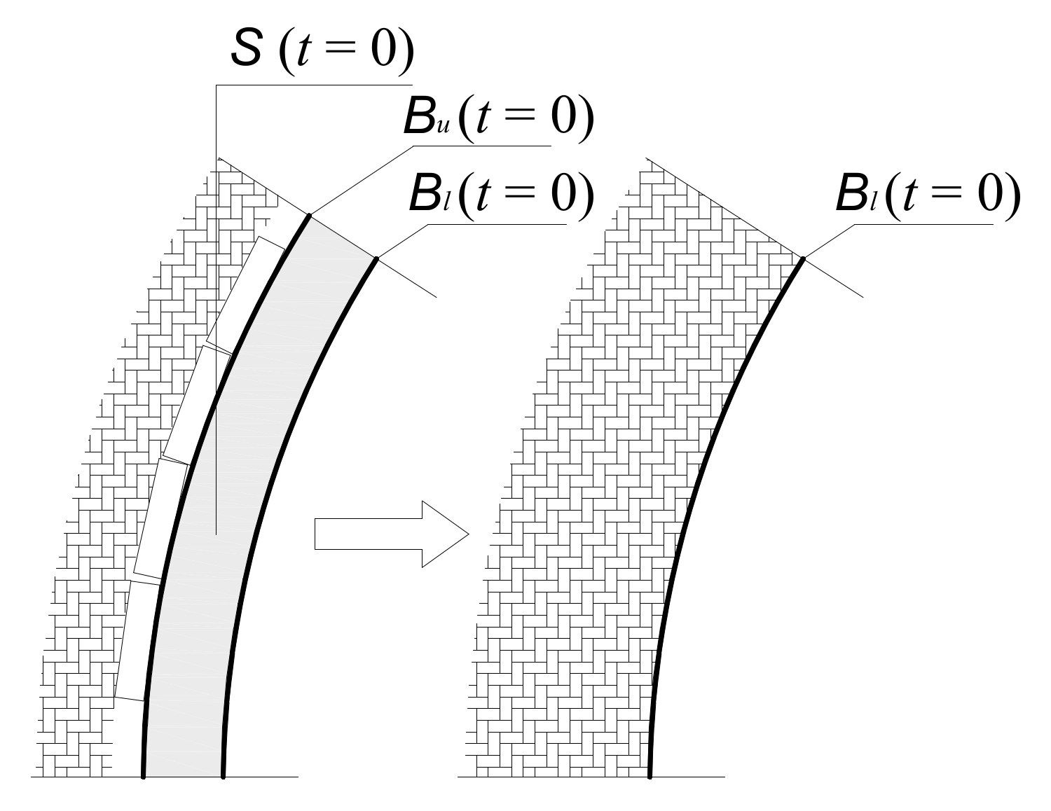
In order to describe deformations of a gate road support, we consider the time dependent displacements only in the vertical cross-section (planar problem). Let S ( t ) be a surface of the support bounded by B ( t ) = [ B l ( t ) , B u ( t ) ] at the current time t, where B l ( t ) represents the lower edge and B u ( t ) represents the upper edge of the support. Without loss of generality, we equal the upper edge with the lower and transform the surface of the support into one line, i.e., we reduce a real two-dimensional support to an artificial one-dimensional support; S ( t = 0 ) R 2 B l ( t = 0 ) R , (Figure 1).
The initial configuration of B l ( t ) , t = 0 is undeformed and known (recorded by laser scanning). The motion of each point on B l ( t ) , t = 0 , from the initial to the current configuration, is completely defined by a time dependent mapping function. Since the equation of this function is unknown and it is necessary to make monitoring of support deformations at equal or nonequal time intervals. Monitoring at equal intervals is much more applicable for forecasting deformations of a gate road. It is very important to use the same coordinate system to describe deformations over the time of monitoring.
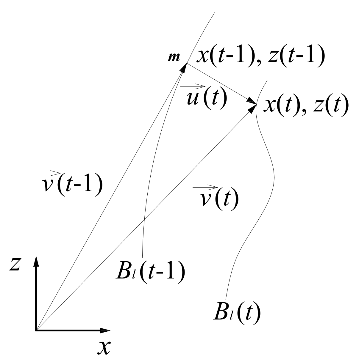
The position of the marker m (   v , t ) , induced by rock stress, changes according to the following vector equation (Figure 2):
v ( t ) = v ( t 1 ) + u ( t ) , t = 1 , 2 , , N   ,
where
  v ( t ) —the position vector of the marker m in the current support configuration.
v ( t - 1 ) —the position vector of the marker m in the previous support configuration.
u   ( t ) —the vector of displacement.
N—time of monitoring.
Figure 2. Change of the marker position over time.
Energies 14 03710 g002
In the xz-coordinate plane, the position of the marker m ( x , z , t ) is defined as follows:
x ( t ) = x ( t 1 ) + Δ x ( t ) z ( t ) = z ( t 1 ) + Δ z ( t ) ,
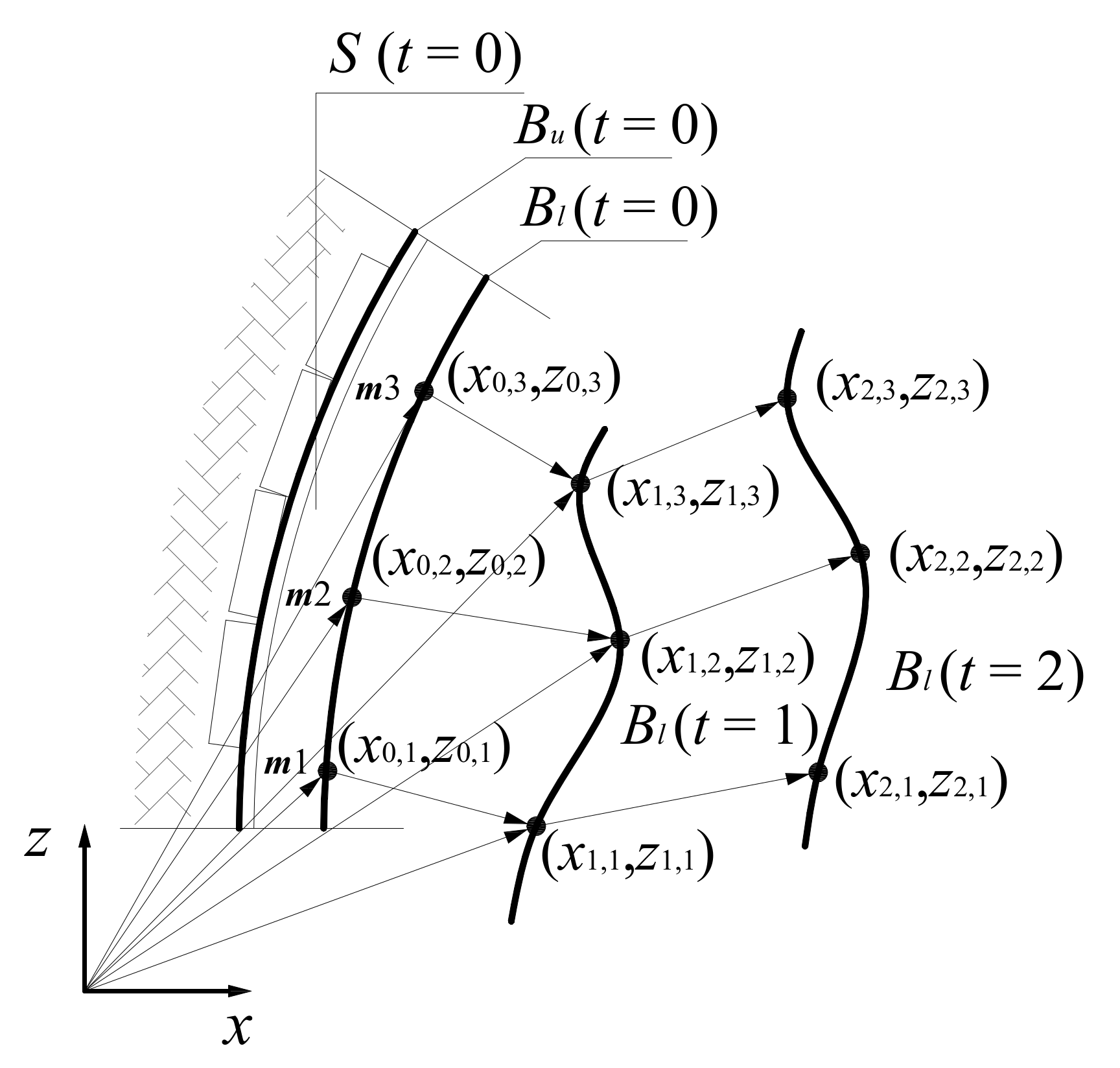
The gate road support domain B l ( t ) is divided into a finite number of segments “connected” at the marker’s position. Support configuration at current time t is defined by the set B l ( t ) = { m t , i } , i = 1 , 2 , , M , where M is the total number of markers. Let us define a section of the initial support configuration by the set D l ( t = 0 ) B l ( t = 0 ) ; D l ( t = 0 ) = { m 0 , 1 , m 0 , 2 , m 0.3 } . At time t = 1 , the section of initial support configuration will be transformed and defined by the set D l ( t = 1 ) = { m 1 , 1 , m 1 , 2 , m 1 , 3 } . At time t = 2 , the topology of the section is defined by the set D l ( t = 2 ) = { m 2 , 1 , m 2 , 2 , m 2 , 3 } . The time-dependent path of the section topology transformation for t = 0 , 1 , 2 is defined as follows: D l ( 0 , 1 , 2 ) = { m 0 , 1 , m 0 , 2 , m 0 , 3 } { m 1 , 1 , m 1 , 2 , m 1 , 3 } { m 2 , 1 , m 2 , 2 , m 2 , 3 } (Figure 3).
In conventional matrix form, the data of position of all markers obtained by scanning for 1 t N can be expressed by the time-dependent position vectors as follows:
V ( t ) = [ v i j ] M × N = [ v 11 v 12 v 13 v 1 N v 21 v 22 v 23 v 2 N v M 1 v M 2 v M 3 v M N ] ,
The position of each marker is represented by each row of the previous matrix, while each column represents the configuration of the gate road support over time. According to Equation (2), x and z coordinates of observed markers are defined as follows:
X ( t ) = [ x i j ] M × N = [ x 11 x 12 x 13 x 1 N x 21 x 22 x 23 x 2 N x M 1 x M 2 x M 3 x M N ] ,
Z ( t ) = [ z i j ] M × N = [ z 11 z 12 z 13 z 1 N z 21 z 22 z 23 z 2 N z M 1 z M 2 z M 3 z M N ] ,
As can be seen, the obtained data can be treated as a multichannel time series. Multivariate singular spectrum analysis is a very useful tool to process such datasets.

2.2. Gateroad Support Deformation Forecasting Algorithm

Our forecasting algorithm is based on the methodology of the multivariate singular spectrum analysis (MSSA). In the paper by Harris and Yuan [12], the basic SSA (singular spectrum analysis) algorithm was presented. Hassani and Zhigljavsky [13] showed that SSA is a powerful method for time-series analysis and forecasting. Hassani and Mahmoudvand [14] pointed out that this method can be applied both to single series and jointly for several series (MSSA). When it is a case of a two or more series, we are talking about MSSA. The application of the SSA technique was found to be very useful for time series analysis in many different fields, such as medicine, biology, genetics, finance, engineering and many others [15]. The basic concept of the singular spectrum analysis is well presented in the paper by Hassani et al. [16].
According to Equation (2), x and z coordinates of the marker m over time correspond to one channel time series. If we take into consideration the total number of markers is M, then we are faced with an M-channel time series.
Consider an M-channel time series with a series length of Ni; V N i ( i ) = ( v 1 ( i ) , , v N i ( i ) ) , ( i = 1 , , M ) , where N is the time of monitoring. Here, we provide the procedure for the x coordinates of the markers. The procedure for the z coordinates is completely the same.
At the first stage of the algorithm, the decomposition, includes the following two steps: embedding and singular value decomposition (SVD) [14,16].
Embedding is a mapping that transfers a one dimensional time series of coordinates X N i ( i ) = ( x 1 ( i ) , , x N i ( i ) ) into a multidimensional matrix [ Y 1 ( i ) , , Y K i ( i ) ] with vectors Y j ( i ) = ( x j ( i ) , , x j + L i + 1 ( i ) ) T R L i , where L i ( 1 < L i < N i ) is the window length for each series with length Ni and K i = N i - L i + 1 . The result of this step is the trajectory matrix Y ( i ) = [ Y 1 ( i ) , , Y K i ( i ) ] = ( y mn ) m , n = 1 L i , K i . The trajectory matrix Y ( i ) is known as a Hankel matrix. Thus, the above procedure for each series separately provides M different L i × K i trajectory matrices Y ( i ) ( i = 1 , , M ) . To form a new block Hankel matrix in a vertical form, we need to have K 1 = = K M = K . The result of this step is the following block Hankel trajectory matrix:
Y V = [ Y ( 1 ) Y ( M ) ] ,
where YV indicates that the output of the first step is a block Hankel trajectory matrix formed in a vertical form; index V means vertical.
In the second step, we perform the SVD of YV. Denote λ V 1 , , λ V L sum as the eigenvalues of Y V Y V T , arranged in decreasing order ( λ V 1 λ V L sum 0 ) and U V 1 , , U V L sum , the corresponding eigenvectors, where L sum = i = 1 M L i . Note also that the structure of the matrix Y V Y V T , is as follows:
Y V Y V T = [ Y ( 1 ) Y ( 1 ) T Y ( 1 ) Y ( 2 ) T Y ( 1 ) Y ( M ) T Y ( 2 ) Y ( 1 ) T Y ( 2 ) Y ( 2 ) T Y ( 2 ) Y ( M ) T Y ( 3 ) Y ( 1 ) T Y ( 3 ) Y ( 2 ) T Y ( 3 ) Y ( M ) T ] ,
The structure of the matrix Y V Y V T is similar to the variance-covariance matrix in the classical multivariate statistical analysis literature. The matrix Y ( i ) Y ( i ) T , which is used in the univariate SSA, for the series X N i ( i ) appears along the main diagonal, and the products of two Hankel matrices Y ( i ) Y ( i ) T ( i j ) that are related to the series X N i ( i ) and X N j ( j ) appear in the off-diagonal. The SVD of Y V can be written as Y V = Y V 1 + + Y V L sum , where Y V i = λ i U V i U V i T and V V i = Y V T U V i / λ V i , ( Y V i = 0 i f λ V i = 0 ) . U V i are called factor empirical orthogonal functions and V V i are the left and right eigenvectors of the trajectory matrix, often called principal components.
The second stage of the algorithm, called reconstruction, includes the following two steps: grouping and diagonal averaging or Hankelization [14,16].
The grouping step corresponds to splitting the matrices Y V 1 , , Y V L sum into several disjointed groups and summing the matrices within each group. The split of the set of indices { 1 , , L sum } into disjointed subsets I 1 , , I k corresponds to the representation of Y V = Y I 1 + + Y I k . The procedure of choosing the sets I 1 , , I k is called grouping. For a given group I, the contribution of the component Y V I is measured by the share of the corresponding eigenvalues: i I λ V i / i = 1 d V λ V i , where dV is the rank of Y V I and I { 1 , , L sum } . In a simple case where we have only signal and noise components, we use two groups of indices, I 1 = { 1 , , r } and I 2 = { r + 1 , , L sum } and associate the group I1 with the signal component and the group I2 with the noise.
The purpose of diagonal averaging is to transform the reconstructed matrix   Y ^ V i into a Hankel matrix, which can subsequently be converted into a time series. Let   Y ˜ ( h ) be the approximation of Y ( i ) obtained from the diagonal averaging step. If   y ˜ mn ( i ) stands for an element of a matrix   Y ˜ ( i ) , then the jth term of the reconstructed series   X ˜ N i ( i ) = (   x ˜ 1 ( i ) , ,   x ˜ j ( i ) , ,   x ˜ N i ( i ) ) is achieved by arithmetic averaging   y ˜ mn ( i ) over all (m, n) such that m + n - 1 = j .
The third stage of the algorithm concerns the future positions of the markers and is based on the vertical multivariate singular spectrum analysis recurrent procedure (VMSSA-R).
Let us have M-channel series X N i ( i ) = ( x 1 ( i ) , , x N i ( i ) ) and corresponding window length Li, 1 < L i N i , i = 1 , , M . Optimal values of the window length are discussed in chapter 4 of the paper by Hassani and Mahmoudvand [14].
The VMSSA-R forecasting algorithm for the h-step ahead forecast is as follows:
For a fixed value of K, construct the trajectory matrix Y ( i ) = [ Y 1 ( i ) , , Y K ( i ) ] = ( y mn ) m , n = 1 L i , K for each single series separately; construct the block trajectory matrix Y V as follows:
Y V = [ Y ( 1 ) Y ( M ) ] ,
let U V j = ( U j ( 1 ) , , U j ( M ) ) T be the jth eigenvector of the Y V Y V T , where U j ( i ) with length Li corresponds to the series X N i ( i ) ( i = 1 , , M ) ; consider   Y ^ V = [   Y ^ 1 : :   Y ^ K ] = i = 1 r U V i U V i T Y V the reconstructed matrix achieved from r eigentriples:
Y ^ V = [ Y ^ ( 1 ) Y ^ ( M ) ] ,
consider matrix   Y ˜ ( i ) = H ×   Y ˜ ( i ) =   Y ˜ ( i ) ( i = 1 , , M ) as the result of the Hankelization procedure of the matrix   Y ˜ ( i ) obtained from the previous step, where is a Hankel operator; assume U j ( i ) denotes the vector of the first L i - 1 components of the vector U j ( i ) and π j ( i ) is the last component of the vector U j ( i ) ( i = 1 , , M ) ; select the number of r eigentriples for the reconstruction stage that can also be used for forecasting purposes; define matrix U M = ( U 1 M , , U r M ) , where U j M is as follows:
U j M = [ U j ( 1 ) U j ( M ) ] ,
define matrix W as follows:
W = [ π 1 ( 1 ) π 2 ( 1 ) π r ( 1 ) π 1 ( 2 ) π 2 ( 2 ) π r ( 2 ) π 1 ( M ) π 2 ( M ) π r ( M ) ] ,
if the matrix ( I M × M - W W T ) - 1 exists and r L sum - M , then the h-step ahead VMSSA forecasts exist and is achieved by the following formula:
[ x ^ j 1 ( 1 ) , , x ^ j M ( M ) ] T = { [ x ˜ j 1 ( 1 ) , , x ˜ j M ( M ) ] , j i = 1 , , N i ( I M × M W W T ) 1 W U M T Z h , j i = N i + 1 , , N i + h ,
where Z h = [ Z h ( 1 ) , , Z h ( M ) ] T and Z h ( 1 ) = [   x ^ N i - L i + h + 1 ( i ) , ,   x ^ N i + h + 1 ( i ) ] ( i = 1 , , M ) . It should be noted that Equation (12) indicates that the h-step ahead forecasts of the refined series are obtained by a multi-dimensional linear recurrent formula (LRF).

2.3. Displacement Time Series Clustering

The time displacement intensity vector of marker m is defined as follows:
Δ v ( t ) = Δ x 2 ( t ) + Δ z 2 ( t ) , t = 1 , 2 , , N ,
The universe of displacement (clustering) is defined as the union of the two following sets:
Δ V = Δ V N i ( i ) Δ V ^ N i + h ( i ) ,
where Δ V N i ( i ) is related to the observed displacement series and Δ   V ^ N i + h ( i ) to the the h-step ahead forecasts of the refined displacement series. Note that clustering is performed for each set separately.
To create the clusters within a defined universe of clustering, we apply the concept of fuzzy time series. Such series, which were first proposed by Song and Chissom, ref. [17] are based on fuzzy set theory proposed by Zadeh [18,19]. The most important advantage of fuzzy time series approaches is to be able to work with a very small set of data and not to require the linearity assumption. In the process of measuring the cross-section of the underground roadways, certain measurement errors can occur (conditioned by the error of the measurement method, instrumental error, personal error by the operator of the instrument, or the error due to the working environment itself), the nature of fuzzy time series is a good choice for a credible presentation of displacements of the markers and its clustering.
Let Δ V M × N be the universe of observed displacement. Data obtained by monitoring can be clustered in different ways, for example, a cluster composed of marker displacement over time separately ( Δ v 12 , Δ v 32 , Δ v 24 , ) , a cluster composed of each row or column data of the matrix ΔV. We focus on each column data in order to see how displacement intensity of configuration of the gate road support changes over time. For that purpose, we apply the concept of fuzzy time series with multiple observations [20,21,22].
A fuzzy set A of Δ V M × N is defined as follows:
A = f A ( Δ v 11 ) Δ v 11 + f A ( Δ v 12 ) Δ v 12 + + f A ( Δ v ^ M N ) Δ v ^ M N ,
where fA is the membership function of A, and f A : Δ V [ 0 , 1 ] . The symbol “+” denotes the union operator. Membership function represents the degree of membership of Δvi in A, where f A ( Δ v i ) [ 0 , 1 ] , 1 i M × N . Let ΔV (t) be the universe of displacement on which fuzzy sets f i ( t ) , ( i = 1 , 2 , ) are defined and F(t) is a collection of f 1 ( t ) , f 2 ( t ) , , F ( t ) that is referred to as a fuzzy time series of ΔV (t). Here, F(t) is viewed as a linguistic variable and f i ( t ) represents possible linguistic values of F(t). If F(t) is caused by F(t – 1) only, the relationship can be expressed as [23]. If the maximum degree of membership of F(t) belongs to Ai then F(t) is considered to be Ai. Hence, F ( t - 1 ) F ( t ) becomes A i ( t - 1 ) A j ( t ) .
The algorithm of a fuzzy time series model for multiple observations is composed of the following steps [23]:
Step 1: define the fuzzy sets for the fuzzy time series. We set the beginning and the end of the universe of displacement as l = min Δ V M × N and u = max Δ V M × N , respectively. The observed data are sorted in ascending order. The distance of any two consecutive values of displacement is calculated as follows:
d = | Δ v i + 1 Δ v i | , i = 1 , 2 , , ( M × N ) 1 ,
Now it is necessary to compute the corresponding average value   d ¯ and standard deviation σ d . The intention is to eliminate the outliers from the sorted data and obtain an average distance value free of distortion. Outliers are values that are either abnormally high or abnormally low in the sorted dataset. The process of elimination of outliers is performed as follows:
d ¯ σ d d d ¯ + σ d ,
Since the process of elimination is completed, a revised average distance value   d ¯ R is calculated for the remaining values in the sorted data set. Accordingly, the universe of displacement is also revised and defined as follows:
Δ V R = [ l R , u R ] = [ l d ¯ R , u + d ¯ R ] ,
The number of equal intervals n is given by the user and each interval is characterized by an adequate linguistic variable. The variable whose values are words or sentences in a natural or artificial language is called a linguistic variable. We use five linguistic variables n = 5 to describe displacement intensity of configuration of the gate road support; A 1 = (very small), A 2 = (small), A 3 = (medium), A 4 = (high), and A 5 = (very high). The length of interval can be calculated by the equation:
L = u R l R n + 1 ,
Each interval is obtained as: Δ v 1 = [ lR , lR + L ] , Δ v 2 = [ lR + L , lR + 2 L ] , , Δ v n = [ l R + ( n 1 ) L , l R + n L ] . Linguistic variable A i ( i = 1 , 2 , , 5 ) can now be defined according to defined intervals as follows:
A 1 = { 1 Δ v 1 , 0.5 Δ v 2 , 0 Δ v 3 , 0 Δ v 4 , 0 Δ v 5 } A 2 = { 0.5 Δ v 1 , 1 Δ v 2 , 0.5 Δ v 3 , 0 Δ v 4 , 0 Δ v 5 } A 3 = { 0 Δ v 1 , 0.5 Δ v 2 , 1 Δ v 3 , 0.5 Δ v 4 , 0 Δ v 5 } A 4 = { 0 Δ v 1 , 0 Δ v 2 , 0.5 Δ v 3 , 1 Δ v 4 , 0.5 Δ v 5 } A 5 = { 0 Δ v 1 , 0 Δ v 2 , 0 Δ v 3 , 0.5 Δ v 4 , 1 Δ v 5 }
The triangular fuzzy number is used to quantify the linguistic variable. It can be defined as a triplet (a, b, c). The corresponding membership function is defined as [24]:
μ A ( Δ v ) = { 0 , Δ v < a Δ v a b a , a Δ v b c Δ v c b , b Δ v c 0 , Δ v > c ,
Step 2: determine a fuzzy observation of displacement. Triangular fuzzy number O ( t ) = ( a ( t ) , b ( t ) , c ( t ) ) is also used to represent displacement of all markers at time point t, where a(t), b(t), c(t) are the left, middle and right values of the triangular fuzzy number, respectively. These values are defined in the following way:
a ( t ) = m i n ( Δ v 1 t , Δ v 2 t , , Δ v M t ) b ( t ) = Δ v 1 t + Δ v 2 t + + Δ v M t M c ( t ) = m a x ( Δ v 1 t , Δ v 2 t , , Δ v M t ) , t = 1 , 2 , , N ,
In other words, for every observation (column of matrix), it is necessary to separate minimum, maximum, and average values of displacement for all markers.
Step 3: calculate the fuzzy relationship, Y(t), between each fuzzified observation and defined fuzzy time series as in Step 1.
Y ( t ) = ( μ 1 ( t ) , μ 2 ( t ) , , μ n ( t ) ) = i = 1 n m a x m i n ( O ( t ) , A i ) , μ i ( t ) 0 ,
Fuzzified observation of displacement at time point t belongs to cluster Ai if and only if their intersection has the highest value of membership function; μ i ( t ) max .
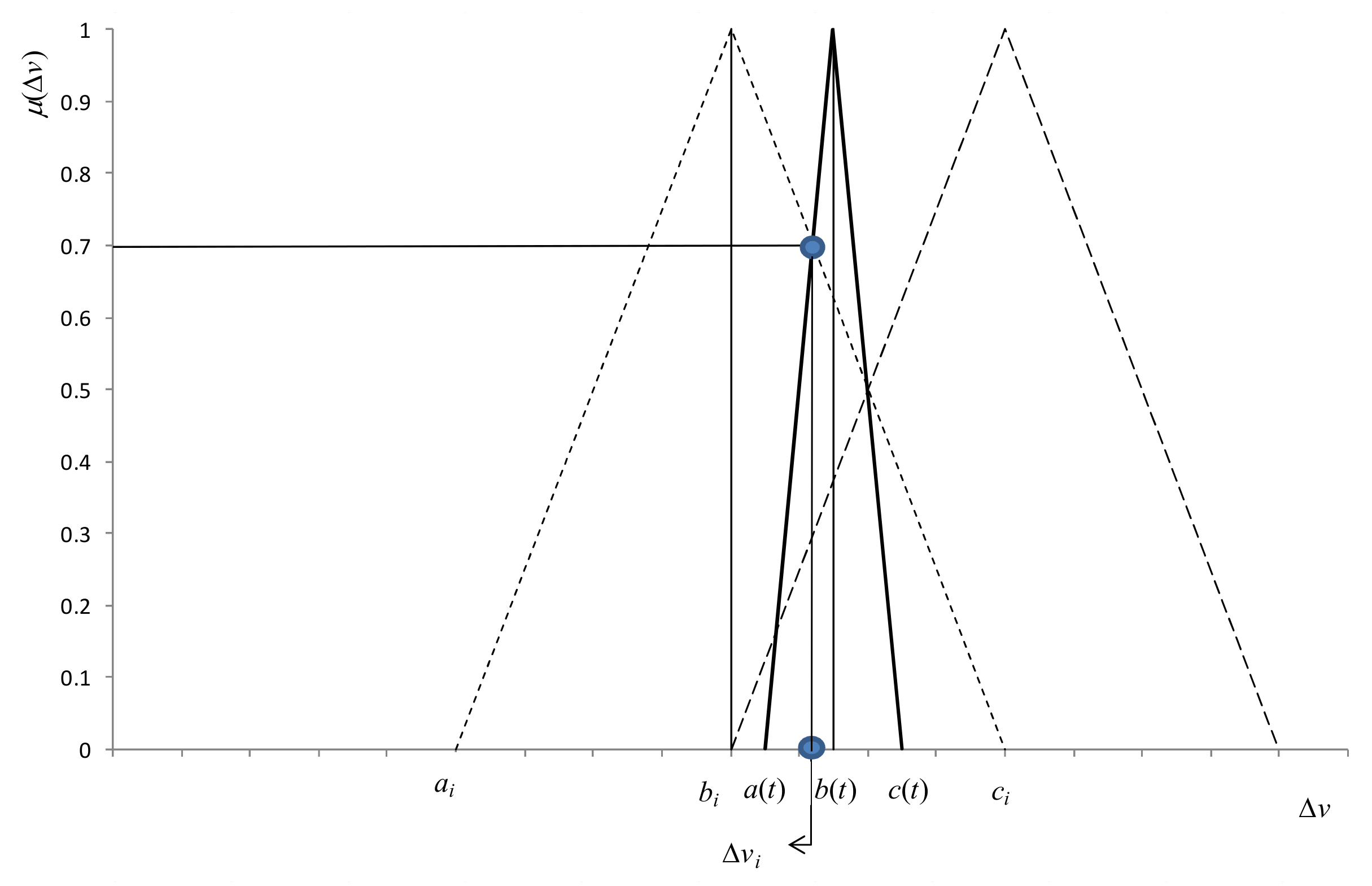
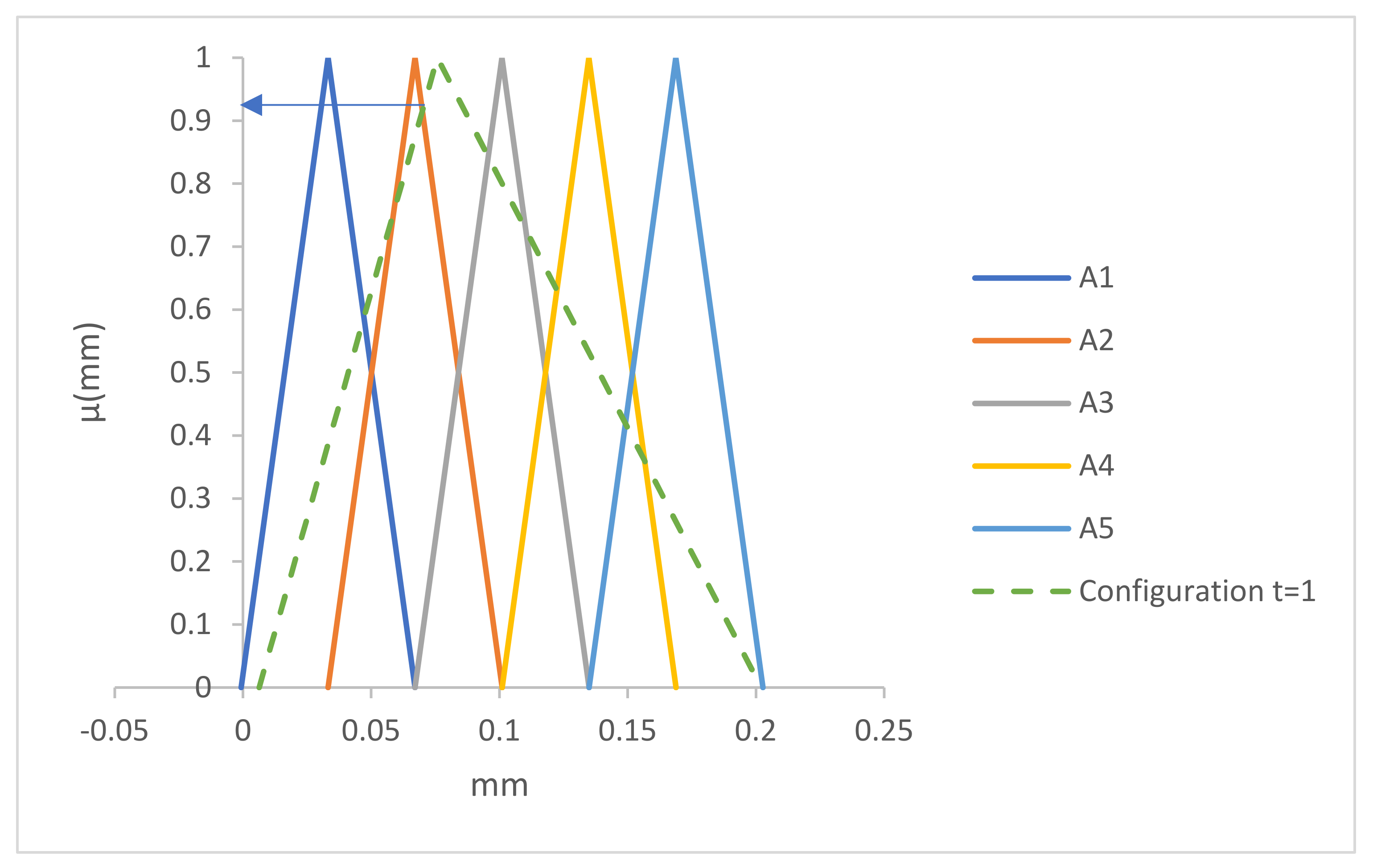
Each μ i ( t ) is calculated according to Figure 4, representing the intersection between a fuzzy observation of displacement O(t) and fuzzy time series consisting of A 1 , A 2 , , A i .
The calculation of the membership function value of intersection is based on the following approach:
1 b ( t ) a ( t ) = μ i ( Δ v i ) Δ v i a ( t ) ,
1 c i b i = μ i ( Δ v i ) c i Δ v i ,
From Equations (24) and (25), we can calculate the value of μ i ( t ) as follows:
μ i ( Δ v i ) = c i a ( t ) b ( t ) a ( t ) + c i b i ,

3. Numerical Example

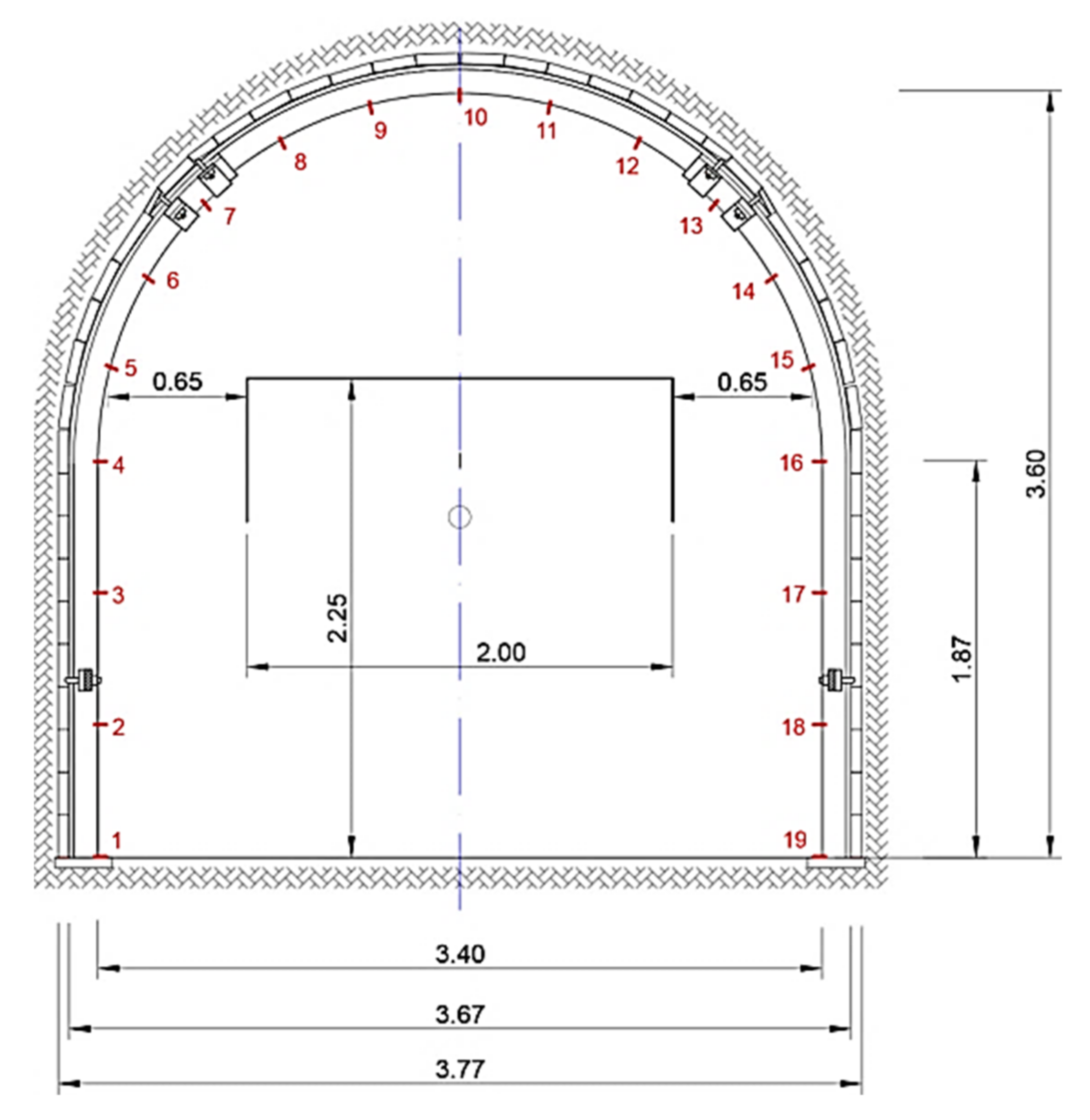
Artificial data related to displacement of markers are generated in order to verify the validity of the proposed forecast model. A cross section of the gate road support and positions of the markers are represented by Figure 5. The coordinate system origin is located at the left lower corner of the gate road support (marker 1). The time resolution of observation is five days.
Coordinate data obtained after six observations are represented in Table 1 and Table 2 and Figure 6.
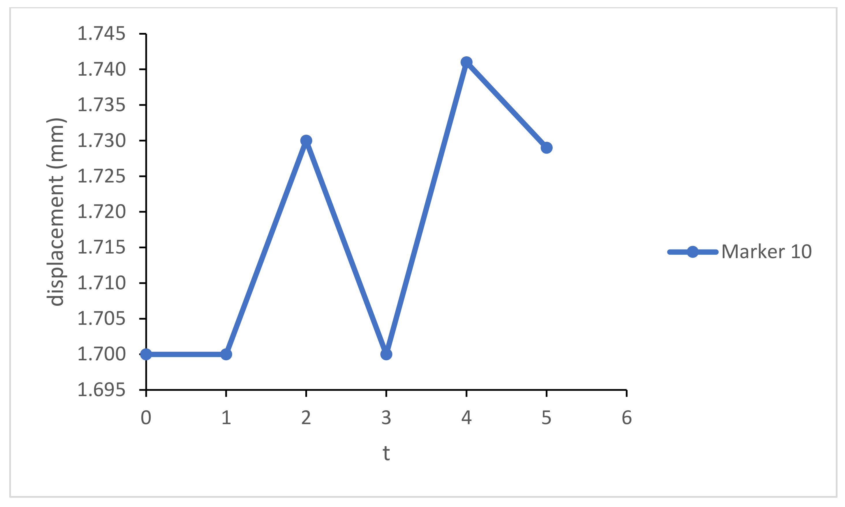
Measurements for t = 0, 1, …, 5 are used to create a forecast model, while the measurement for t = 6 is used as a control series. Detail calculation is provided for the x coordinates. Figure 7 represents x coordinates of the marker 10 obtained by observation.
The inputs needed to perform multivariate singular spectrum analysis are:
  • the number of markers (series) M = 19,
  • the time series length needs to be equal to each marker (series) N = 6,
  • the window length for each marker (series) L = 3,
  • parameter K also needs to be equal to each marker (series) K = 4.
The trajectory matrix of marker 1 is obtained as follows: from the original series X(1) = (0.000 0.011 0.025 0.039 0.055 0.068), we create the following trajectory matrix of dimension L × K = 3 × 4 .
Y ( 1 ) = [ 0.000 0.011 0.025 0.039 0.011 0.025 0.039 0.055 0.025 0.039 0.055 0.068 ] ,
The above procedure is performed for each series separately and provides nineteen different L × K = 3 × 4 trajectory matrices Y ( i ) ( i = 1 , 2 , , 19 ) . The result of this step is the following vertical formed block Hankel trajectory matrix:
Y V = [ Y ( 1 ) Y ( 2 ) Y ( 19 ) ] = [ 0.000 0.011 0.025 0.039 0.011 0.025 0.039 0.055 0.025 0.039 0.055 0.068 0.000 0.019 0.035 0.053 0.019 0.035 0.053 0.071 0.035 0.053 0.071 0.085 3.400 3.391 3.379 3.365 3.391 3.379 3.365 3.351 3.379 3.365 3.351 3.341 ] ,
The eigenvalues of Y V Y V T , arranged in decreasing order are λ V 1 = 1066.7105 ; λ V 2 = 0.2704 ; λ V 3 = 0.0135 ; λ V 4 = 0.0080 . The values of the corresponding eigenvectors U V 1 , U V 2 , U V 3 , U V 4 are represented in Table 3.
The rank of the matrix Y V is d = 4 . The contribution of the component Y V I is measured by the share of the corresponding eigenvalues (Table 4).
To perform the reconstruction stage, it is necessary to calculate the principal components V V i = Y V T U V i / λ V i . The results of this calculation are represented in Table 5.
The reconstructed trajectory matrix of all markers achieved from four eigentriples is presented in Table 6.
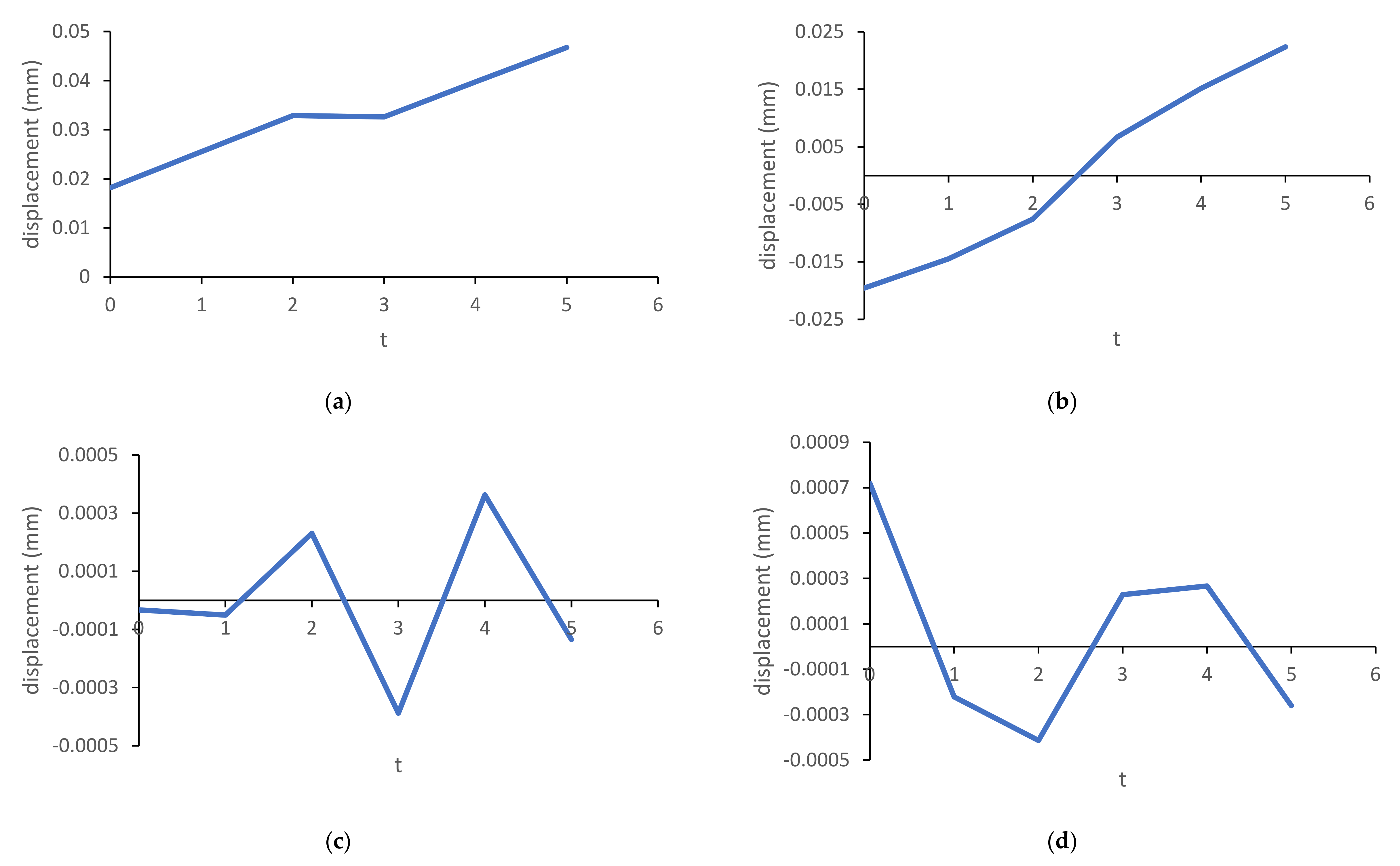
The reconstructed series of marker M1 expressed in the form of principal components achieved by arithmetic averaging of   Y ^ V 1 ( 1 ) ,   Y ^ V 2 ( 1 ) ,   Y ^ V 3 ( 1 ) ,   Y ^ V 4 ( 1 ) are represented in Table 7 and Figure 8 separately.
Within the grouping step, we only have signal and noise components and we use two groups of indices, I 1 = { λ V 1 , λ V 2 } and I 2 = { λ V 3 , λ V 4 } and associate the group I1 with signal component and the group I2 with noise. The reconstructed series of x coordinates of the marker M1 composed of the signal components are represented in Table 8.
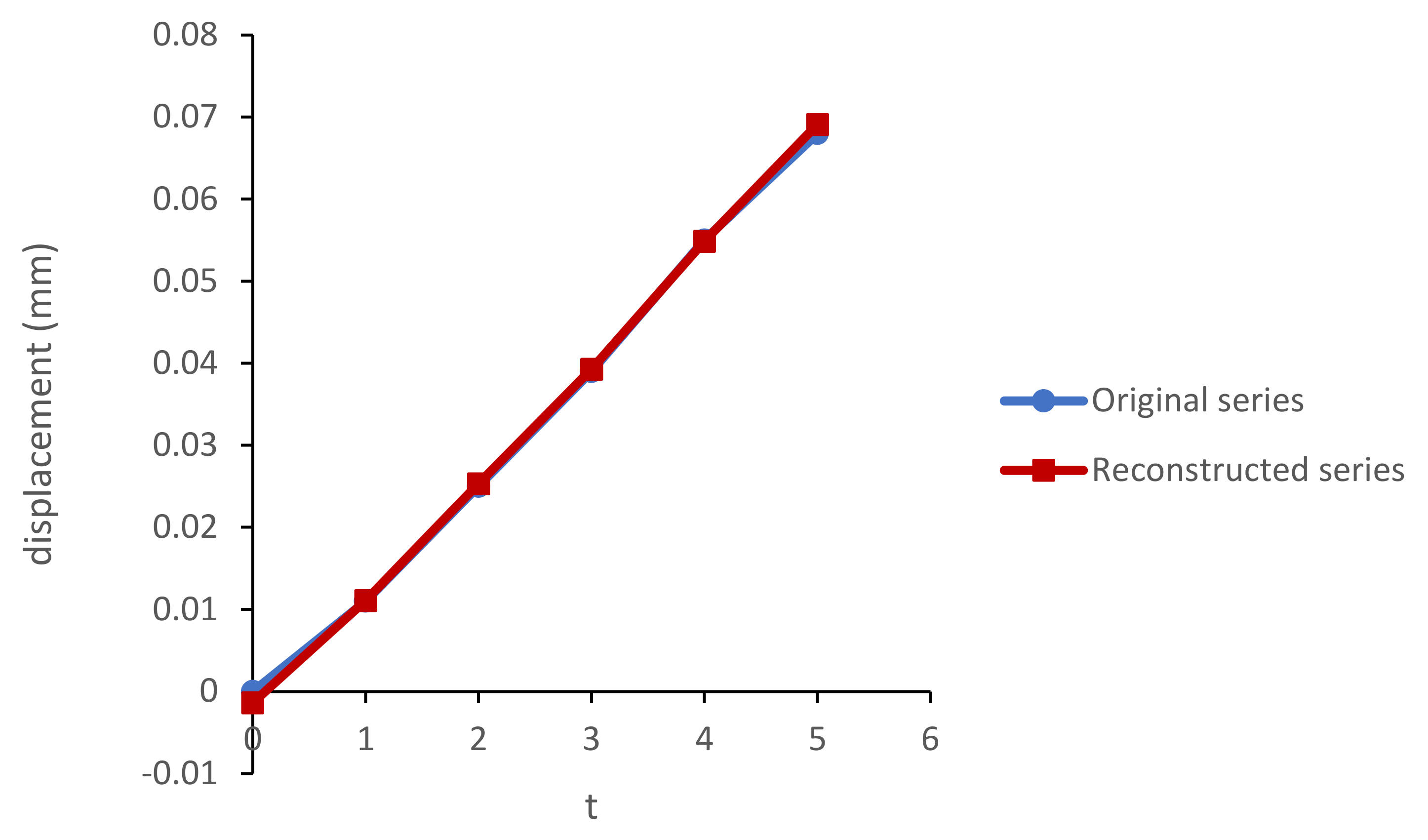
Figure 9 represents the original and reconstructed series of x coordinates of the marker M1 using only signal group (I1).
The reconstructed series   X ˜ N i ( i ) , i = 1 , 2 , , 19 achieved by arithmetic averaging of Y V ( I 1 ) are represented in Table 9.
The error of the reconstruction stage is calculated according to the following equation of mean absolute percentage error (MAPE):
M A P E i = 1 N N i = 1 N | X ˜ N i ( i ) X N i ( i ) X N i ( i ) | × 100 % ,
The aggregated mean absolute percentage error (AMAPE) of the reconstruction stage is calculated as follows:
A M A P E = 1 M i = 1 M M A P E i ,
MAPEi and AMAPE are represented in Table 10.
Signal components used for the reconstruction stage were also used for the forecasting purpose. Vector U j ( i ) , j = 1 , 2 , composed of the first L i - 1 components of the vector U j ( i ) , j = 1 , 2 , 3 , 4 , is represented in Table 11.
Vector π j ( i ) , j = 3 , composed of the last component of the vector U j ( i ) , ( i = 1 , , M ) , is represented in Table 12.
Forecasted x coordinates of the markers for h = 1 step ahead are obtained according to Equation (12) and represented in Table 13.
The analogous procedure is performed for z coordinates. The reconstructed series   Z ˜ N i ( i ) , i = 1 , 2 , , 19 are represented in Table 14.
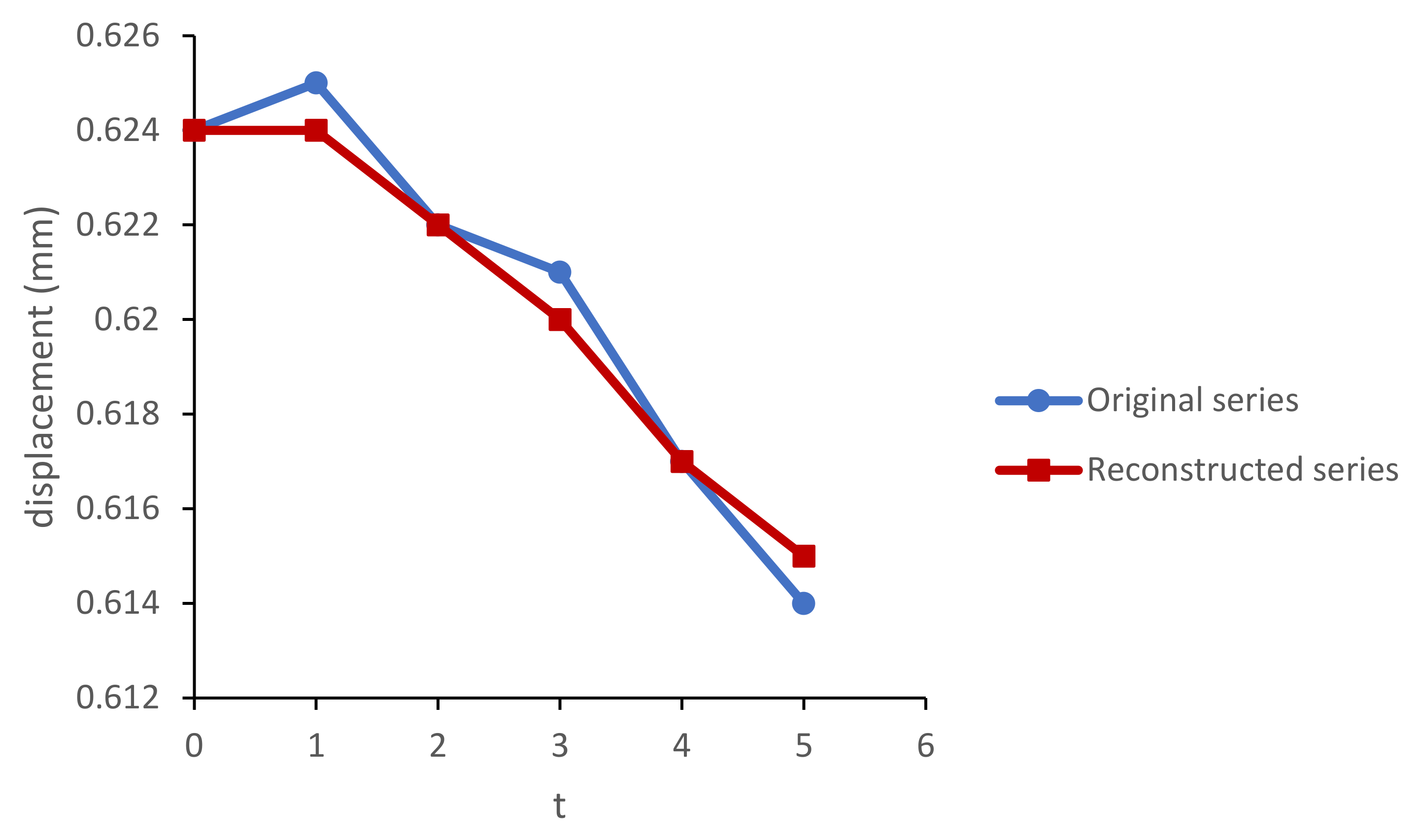
The difference between the original and reconstructed series for marker 2 is represented in Figure 10.
Aggregated mean absolute percentage error (AMAPE) of reconstruction stage of z coordinates is 0.18%. Forecasted z coordinates of the markers for h = 1 step ahead are obtained according to Equation (12) and represented in Table 15.
The time displacement intensity vector of marker m for t = 0, 1, …, 5 and t = 6, 7, 8 is represented in Table 16.
The universe of displacement is defined as follows: D = [ l , u ] , where l = min Δ V 19 × 19 = 0 and u = max Δ V 19 × 19 = 0.2020 . The observed and forecasted data are sorted in the following ascending order: 0, 0, …, 0.0063, 0.0090,…,0.1958, and 0.2020. The distance of any two consecutive values is: 0, 0, …, 0.0027,…,0.0062. The corresponding average value   d ¯ and standard deviation σ d of obtained distances are: d ¯ = 0.0011 , σ d = 0.0038 . The process of elimination of outliers is performed with respect to the following condition: - 0.00265 d 0.00503 . A revised average distance is d ¯ R = 0.000695 . A revised universe of displacement is Δ V R = [ 0.0007 , 0.2027 ] . According to Equation (19) the length of interval is 0.0338.
Quantification of the linguistic variables by the triangular fuzzy numbers is represented in Table 17.
According to Equation (22), displacement intensity of configuration of the gate road support for t = 1 is: O ( 1 ) = ( a ( 1 ) , b ( 1 ) , c ( 1 ) ) = ( 0.0632 , 0.0758 , 0.2020 ) (Figure 11).
Fuzzy relationships between fuzzified observation O ( 1 ) = ( a ( 1 ) , b ( 1 ) , c ( 1 ) ) for t = 1 and defined fuzzy time series are: μ A 1 ( 1 ) = 0.587 ; μ A 2 ( 1 ) = 0.754 ; μ A 2 ( 1 ) = 0.915 ; μ A 3 ( 1 ) = 0.842 ; μ A 3 ( 1 ) = 0.727 ; μ A 4 ( 1 ) = 0.631 ; μ A 4 ( 1 ) = 0.359 ; μ A 5 ( 1 ) = 0.419 ; μ A 5 ( 1 ) = 0 . Fuzzified observation of displacement intensity of configuration of the gate road support for t = 1 belongs to the cluster A2 because the intersection between O(1) and A2 has the highest value of membership function, μ A 2 ( 1 ) = 0.915 , (Figure 11).

4. Results

Finally, the obtained sequences of displacement intensity of configuration of the gate road support over observed and forecasted time is as follows: A2→A2→A2→A2→A2→A1→A1→A1, see Figure 12.

5. Conclusions

Efficiency of underground mine production directly depends on functionality of the main gate roads. Due to hard geological conditions and mining activities, deformations of gate roads are very intensive and happen frequently. Having the ability to monitor and forecast deformations is recognized as a key role to maintaining the stability of gate roads, i.e., to maintain their functionality. The signal and noise of deformations are isolated by multivariate singular spectrum analysis and it is also used to forecast future deformations with respect to different combinations of obtained principal components. Clustering based on fuzzy time series enables us to see how the configuration of the gate road support has generally changed over time and defines the intervals of deformation by adequate triangular fuzzy numbers. Making decisions and plans based on the intervals is much more reliable and suitable than performing such activities based on crisp values.
The developed model enables mine planners to create an effective plan to support repairs, including duration time and costs of reparation with respect to forecasted deformations. Future research will be focused on carrying an in situ measuring of the deformations in an underground mine to quantify the quality of the method. Furthermore, the focus will be on the making of a 3-D model of gate road support deformation forecasting.

Author Contributions

Conceptualization, R.T.; software, A.G.; formal analysis, S.L.; writing—original draft preparation, L.C.; visualization, A.M.; supervision, Z.G. All authors have read and agreed to the published version of the manuscript.

Funding

This research received no external funding.

Institutional Review Board Statement

Not applicable.

Informed Consent Statement

Not applicable.

Data Availability Statement

Not applicable.

Conflicts of Interest

The authors declare no conflict of interest.

References

  1. Xu, D.P.; Feng, X.T.; Cui, Y.J.; Jiang, Q. Use of the equivalent continuum approach to model the behaviour of a rock mass containing an interlayer shear weakness zone in an underground cavern excavation. Tunn. Undergr. Space Technol. 2015, 47, 35–51. [Google Scholar] [CrossRef]
  2. Armaghani, D.J.; Mohamad, E.T.; Hajihassani, M.; Yagiz, S.; Motaghedi, H. Application of several non-linear prediction tools for estimating uniaxial compressive strength of granitic rocks and comparison of their performances. Eng. Comput. 2016, 32, 189–206. [Google Scholar] [CrossRef]
  3. Xiong, X. Research on Grey System Model and its Application on Displacement Prediction in Tunnel Surrounding Rock. Open Mech. Eng. J. 2014, 8, 514–518. [Google Scholar] [CrossRef]
  4. Tang, P. Forecast the Working Face Underground Pressure Using Grey Model Improved by the Genetic Algorithm. Electron. J. Geotech. Eng. 2011, 16, 1215–1226. [Google Scholar]
  5. Yu, S.; Hongzhen, Z.; Yanna, C. Application of GRNN in Time Series Prediction for Deformation of Surrounding Rocks in Soft Rock Roadway. In Proceedings of the 2011 Fourth International Conference on Intelligent Computation Technology and Automation, Shenzhen, China, 28–29 March 2011; Volume 1, pp. 63–66. [Google Scholar]
  6. Chen, H.; Wang, R. Artificial Neural Network’s Application in Intelligent Displacement Back Analysis of Deep Mine Roadway Surrounding Rock. In Proceedings of the 2010 International Conference on Intelligent Computation Technology and Automation, Changsha, China, 11–12 May 2010; Volume 1, pp. 808–811. [Google Scholar]
  7. Bozzano, F.; Mazzanti, P.; Prestininzi, A. Supporting Tunnelling Excavation of an Unstable Slope by Long term Displacement Monitoring. In Proceedings of the International Conference on Case Histories in Geotechnical Engineering, Chicago, IL, USA, 29 April–4 May 2013; p. 42. [Google Scholar]
  8. Zhang, Q.; Li, S.C.; Li, L.P.; Zhang, Q.Q.; Shi, S.S.; Song, S.G. Numerical Analysis of Advanced Displacement in Construction Progress of Tunnel Excavation with Weak Surrounding Rock. Res. J. Appl. Sci. Eng. Technol. 2013, 6, 1497–1503. [Google Scholar] [CrossRef] [Green Version]
  9. Grossauer, K.; Leitner, R.; Schubert, W.; Sellner, P. Prediction of subsidence during tunnel construction. In Underground Space—The 4th Dimension of Metropolises, Proceedings of the 33rd ITA-AITES World Tunnel Congress; Prague, Czech Republic, 5–10 May 2007, Barták, J., Hrdina, I., Romancov, G., Zlámal, J., Eds.; Taylor & Francis Group: London, UK, 2007; pp. 857–862. [Google Scholar]
  10. Merlini, D.; Falanesca, M. Ceneri Base Tunnel advancement in difficult rock conditions: Tunnel design and construction optimization through back-analysis of the geomechanical parameters. In Proceedings of the World Tunnel Congress 2013 Geneva Underground—The Way to the Future, Geneva, Switzerland, 31 May–7 June 2013; Anagnostou, G., Ehrbar, H., Eds.; Taylor & Francis Group: London, UK, 2013; pp. 1722–1729. [Google Scholar]
  11. Yao, B.Z.; Yang, C.Y.; Yao, J.B.; Sun, J. Tunnel Surrounding Rock Displacement Prediction Using Support Vector Machine. Int. J. Comput. Intell. Syst. 2010, 3, 843–852. [Google Scholar] [CrossRef]
  12. Harris, T.J.; Yuan, H. Filtering and frequency interpretations of Singular Spectrum Analysis. Phys. D 2010, 239, 1958–1967. [Google Scholar] [CrossRef]
  13. Hassani, H.; Zhigljavsky, A. Singular Spectrum Analysis: Methodology and Application to Economics Data. J. Syst. Sci. Complex. 2009, 22, 372–394. [Google Scholar] [CrossRef]
  14. Hassani, H.; Mahmoudvand, R. Multivariate Singular Spectrum Analysis: A General View and New Vector Forecasting Approach. Int. J. Energy Stat. 2013, 1, 55–83. [Google Scholar] [CrossRef]
  15. Kalantari, M.; Hassani, H. Automatic Grouping in Singular Spectrum Analysis. Forecasting 2019, 1, 189–204. [Google Scholar] [CrossRef] [Green Version]
  16. Hassani, H.; Yeganegi, M.R.; Silva, E.S. A New Signal Processing Approach for Discrimination of EEG Recordings. Stats 2018, 1, 155–168. [Google Scholar] [CrossRef] [Green Version]
  17. Song, Q.; Chissom, B.S. Fuzzy time series and its models. Fuzzy Sets Syst. 1993, 54, 269–277. [Google Scholar] [CrossRef]
  18. Zadeh, L.A. Fuzzy sets. Inform. Control 1965, 8, 338–353. [Google Scholar] [CrossRef] [Green Version]
  19. Zadeh, L.A. The Concept of a Linguistic Variable and its Application to Approximate Reasoning. In Learning Systems and Intelligent Robots; Fu, K.S., Tou, J.T., Eds.; Springer: Boston, MA, USA, 1974. [Google Scholar] [CrossRef]
  20. Huarng, K.H.; Hui, T.; Yu, K. Modelling fuzzy time series with multiple observations. Int. J. Innov. Comput. Inf. Control 2012, 8, 7415–7426. [Google Scholar]
  21. Chen, S.M. Forecasting enrolments based on fuzzy time series. Fuzzy Sets Syst. 1996, 81, 311–319. [Google Scholar] [CrossRef]
  22. Liang, C.T.; Hsue, C.C.; Ching, C.Y. Using Extracted Fuzzy Rules Based on Multi-Technical Indicators for Forecasting TAIEX. In Proceedings of the International Conference on Artificial Intelligence (ICAI’10), Las Vegas, NV, USA, 12–15 July 2010; pp. 30–34. [Google Scholar]
  23. Su, C.H.; Chen, T.L.; Cheng, C.H.; Chen, Y.C. Forecasting the Stock Market with Linguistic Rules Generated from Minimize Entropy Principle and the Cumulative Probability Distribution Approaches. Entropy 2010, 12, 2397–2417. [Google Scholar] [CrossRef]
  24. Kaufmann, A.; Gupta, M.M. Introduction to Fuzzy Arithmetic: Theory and Applications; Van Nostrand Reinhold: New York, NY, USA, 1985. [Google Scholar]
Figure 1. Transformation of real two-dimensional support to an artificial one-dimensional support.
Energies 14 03710 g001
Figure 3. Change of the section of support configuration over time interval [0, 2].
Energies 14 03710 g003
Figure 4. Relationship between fuzzy observation and fuzzy time series.
Energies 14 03710 g004
Figure 5. Gate road cross section with marker positions.
Energies 14 03710 g005
Figure 6. Configuration of the gate road support over the time of observation.
Energies 14 03710 g006
Figure 7. x coordinates of marker 10.
Energies 14 03710 g007
Figure 8. The reconstructed series of x coordinates of the marker M1 decomposed on principal components: (a) the first principal component 99.9726%; (b) the second principal component 0.02534%; (c) the third principal component 0.00126%; (d) the fourth principal component 0.00075%.
Energies 14 03710 g008
Figure 9. Original and reconstructed series of x coordinates of M1.
Energies 14 03710 g009
Figure 10. Original and reconstructed series of z coordinates of M2.
Energies 14 03710 g010
Figure 11. Fuzzy relationships between O(1) and A1, A2, A3, A4, and A5.
Energies 14 03710 g011
Figure 12. Topology of the gate road support over time, blue color-observed and red color-forecasted configuration.
Energies 14 03710 g012
Table 1. X coordinates of the markers (m).
Markert = 0t = 1t = 2t = 3t = 4t = 5
1 X(1)0.0000.0110.0250.0390.0550.068
2 X(2)0.0000.0190.0350.0530.0710.085
3 X(3)0.0000.0220.0470.0790.1040.135
4 X(4)0.0000.0300.0720.1110.1530.207
5 X(5)0.0580.0950.1320.1920.2300.281
6 X(6)0.2330.2580.3400.3840.4730.517
7 X(7)0.5020.5490.6300.6460.7200.732
8 X(8)0.8590.8760.9270.9341.0101.038
9 X(9)1.2781.2991.3601.3511.3081.343
10 X(10)1.7001.7001.7301.7001.7411.729
11 X(11)2.1222.0892.1192.0792.0542.027
12 X(12)2.5412.5212.4682.4492.4472.408
13 X(13)2.8982.8302.8142.7262.7212.665
14 X(14)3.1673.1083.0803.0312.9952.903
15 X(15)3.3423.3003.2603.1843.1203.081
16 X(16)3.4003.3723.3393.2873.2573.226
17 X(17)3.4003.3873.3643.3413.3133.286
18 X(18)3.4003.3943.3763.3573.3413.326
19 X(19)3.4003.3913.3793.3653.3513.341
Table 2. Z coordinates of the markers (m).
Markert = 0t = 1t = 2t = 3t = 4t = 5
1 Z(1)0.0000.0000.0000.0000.0000.000
2 Z(2)0.6240.6250.6220.6210.6170.614
3 Z(3)1.2451.2311.2391.2211.2351.219
4 Z(4)1.8601.8461.8531.8351.8261.823
5 Z(5)2.3052.2842.2662.2662.2632.269
6 Z(6)2.7232.6692.6102.6152.5792.549
7 Z(7)3.0722.9982.9162.8992.8512.843
8 Z(8)3.3713.2613.1883.1333.0572.982
9 Z(9)3.5383.3863.2513.1633.1013.044
10 Z(10)3.5903.3883.3083.2073.1263.026
11 Z(11)3.5373.3443.2583.1243.0312.930
12 Z(12)3.3713.2193.1463.0793.0172.936
13 Z(13)3.0722.9392.8902.8152.7782.730
14 Z(14)2.7232.6622.6342.6062.5872.552
15 Z(15)2.3052.2712.2412.2392.2192.209
16 Z(16)1.8601.8531.8441.8391.8201.812
17 Z(17)1.2451.2411.2381.2491.2441.242
18 Z(18)0.6240.6220.6210.6200.6200.622
19 Z(19)0.0000.0000.0000.0000.0000.000
Table 3. Corresponding eigenvectors of Y V Y V T .
MarkerUV1UV2UV3UV4
10.0011−0.0570−0.0017−0.0151
0.0020−0.0639−0.0113−0.0075
0.0029−0.06400.00380.0064
20.0016−0.0761−0.01630.0108
0.0027−0.0764−0.0050−0.0085
0.0037−0.07440.00270.0238
190.2072−0.0705−0.02680.0102
0.2065−0.0628−0.0298−0.0064
0.2057−0.0649−0.0375−0.0386
Table 4. Share of the eigenvalues.
Eigenvalue i I λ V i / i = 1 4 λ V i Share (%)
λ V 1 = 1066.7105 1066.7105/1067.002499.9726
λ V 2 = 0.2704 0.2704/1067.00240.02534
λ V 3 = 0.0135 0.0135/1067.00240.00126
λ V 4 = 0.0080 0.0080/1067.00240.00075
Sum: 1067.0024
Table 5. Values of V V i .
V V 1
V V 2
V V 3
V V 4
0.50612090.65966380.1650227−0.5318409
0.50200780.2372012−0.58174020.5924250
0.4982835−0.23961310.73594430.3984461
0.4935079−0.6718575−0.3059158−0.4548699
Table 6. Reconstructed trajectory matrix of Y ^ V .
Y ^ V 1 ( i ) , i = 1 , 2 , , 19 Y ^ V 2 ( i ) , i = 1 , 2 , , 19 Y ^ V 3 ( i ) , i = 1 , 2 , , 19 Y ^ V 4 ( i ) , i = 1 , 2 , , 19
0.018180.018040.017900.01773−0.01955−0.007030.007100.01991−0.000030.00011−0.000150.000060.00072−0.00080−0.000540.00061
0.033060.032790.032550.03224−0.02192−0.007880.007960.02232−0.000220.00076−0.000970.000400.00036−0.00040−0.000270.00031
0.047940.047550.047200.04674−0.02195−0.007890.007970.022360.00007−0.000260.00032−0.00014−0.000300.000340.00023−0.00026
0.026450.026230.026040.02579−0.02610−0.009390.009480.02659−0.000310.00110−0.001390.00058−0.000510.000570.00038−0.00044
0.044630.044270.043940.04352−0.02621−0.009420.009520.02669−0.000100.00034−0.000430.000180.00040−0.00045−0.000300.00035
0.061160.060660.060210.05964−0.02552−0.009180.009270.025990.00005−0.000180.00023−0.00010−0.001130.001260.00085−0.00097
3.425053.397223.372023.33970−0.02418−0.008700.008780.02463−0.000510.00181−0.002290.00095−0.000490.000540.00036−0.00041
3.413483.385743.360623.32842−0.02154−0.007750.007820.02194−0.000570.00201−0.002550.001060.00030−0.00034−0.000230.00026
3.400263.372633.347603.31552−0.02226−0.008010.008090.02267−0.000720.00253−0.003210.001330.00184−0.00205−0.001380.00157
Table 7. Reconstruction stage of principal components of marker M1.
x ˜ 0 ( 1 ) x ˜ 1 ( 1 ) x ˜ 2 ( 1 ) x ˜ 3 ( 1 ) x ˜ 4 ( 1 ) x ˜ 5 ( 1 )
X ˜ V 1 ( 1 ) 0.01818320.02554790.03287690.03260880.03971580.0467429
X ˜ V 2 ( 1 ) −0.0195524−0.0144750−0.00757770.00666060.01514940.0223594
X ˜ V 3 ( 1 ) −0.0000326−0.00005090.0002304−0.00038760.0003633−0.0001351
X ˜ V 4 ( 1 ) 0.0007183−0.0002217−0.00041330.00022870.0002666−0.0002604
Table 8. The reconstructed series of the marker M1 composed of the signal components.
x ˜ 0 ( 1 ) x ˜ 1 ( 1 ) x ˜ 2 ( 1 ) x ˜ 3 ( 1 ) x ˜ 4 ( 1 ) x ˜ 5 ( 1 )
X ˜ V 1 ( 1 ) + X ˜ V 2 ( 1 ) −0.0013690.0110730.0252990.0392690.0548650.069102
Table 9. Reconstructed series of x coordinates of markers based on the signal components.
Markert = 0t = 1t = 2t = 3t = 4t = 5
1 X(1)−0.0010.0110.0250.0390.0550.069
2 X(2)0.0000.0180.0350.0520.0700.086
19 X(19)3.4013.3903.3793.3663.3533.338
Table 10. Error of reconstruction stage.
Marker M A P E i ( 0 ) M A P E i ( 1 ) M A P E i ( 2 ) M A P E i ( 3 ) .   M A P E i ( 4 ) M A P E i ( 5 ) M A P E i ( % )
10.140.661.200.690.251.620.76
20.037.180.961.051.620.741.93
190.030.020.000.020.060.080.04
AMAPE 0.95
Table 11. Components of the vector U j ( i ) , j = 1 , 2 .
MarkerUV1UV2
10.0011−0.0570
0.0020−0.0639
20.0016−0.0761
0.0027−0.0764
190.2072−0.0705
0.2065−0.0628
Table 12. Components of the vector π j ( i ) , j = 3 .
MarkerUV1UV2
10.0029−0.0640
20.0037−0.0744
190.2057−0.0649
Table 13. Forecasted x coordinates for h = 1.
Markert = 6t = 7t = 8
10.0830.0960.108
20.1020.1170.131
193.3233.3033.281
Table 14. Reconstructed series of Z coordinates of markers based on the signal components.
Marker t = 0t = 1t = 2t = 3t = 4t = 5
1 Z(1)0.0000.0000.0000.0000.0000.000
2 Z(2)0.6240.6240.6220.6200.6170.615
19 Z(19)0.0000.0000.0000.0000.0000.000
Table 15. Forecasted z coordinates for h = 1.
Markert = 6t = 7t = 8
10.0000.0000.000
20.6120.6110.609
....
190.0000.0000.000
Table 16. Displacement intensity vector ΔV.
MarkerΔv(t = 0)Δv(t = 1)Δv(t = 2)Δv(t = 3)Δv(t = 4)Δv(t = 5)Δv(t = 6)Δv(t = 7)Δv(t = 8)
10.0000.0110.0140.0140.0160.0130.0150.0130.012
20.0000.0190.0160.0180.0180.0140.0170.0150.015
190.0000.0090.0120.0140.0140.0100.0180.0200.022
Table 17. Variables obtained by quantification.
Variableaibici
A1−0.00070.03320.0671
A20.03320.06710.1010
A30.06710.10100.1349
A40.10100.13490.1688
A50.13490.16880.2027
Publisher’s Note: MDPI stays neutral with regard to jurisdictional claims in published maps and institutional affiliations.