Vector Modulation-Based Model Predictive Current Control with Filter Resonance Suppression and Zero-Current Switching Sequence for Two-Stage Matrix Converter

Abstract

This paper proposes a novel model predictive current control scheme for two-stage matrix converter. The switching frequency is kept constant by fixing the switching instant. The control strategy achieves to control source reactive power in the input side and output currents in the output side. In addition, the advantage of the proposed strategy compared with conventional model predictive control is firstly proved using the principle of vector synthesis and the law of sines in the vector distribution area. Moreover, a zero-current switching sequence is proposed and implemented to insure zero-current switching operations and reduce the switching losses. Furthermore, in order to suppress the input filter resonance, which is easier to be inspired by the model predictive control, compared with traditional control strategies, an innovative active damping technique is proposed and implemented. Finally, both simulation and experiment are implemented to verify the performance of the proposed strategy. The results demonstrate that the control system features both good steady and transient performance.

1. Introduction

Matrix converters (MC) can offer direct AC–AC power conversion with no use of DC-link capacitors and have often been studied as an alternative to the traditional power topologies [1,2]. The most known MC topologies are named one-stage matrix converter (OSMC) and two-stage matrix converter (TSMC), which have the same transfer function [3,4]. The converter family has been globally discussed in all respects of control schemes, power topologies and trends in recent years [5,6,7]. The space vector modulation (SVM) method has been a mature technique for MC, in which both the input and output voltages and currents are considered using space vectors [8,9,10,11], whereas model predictive control (MPC) defies SVM with the emergence of developing digital processors and power devices [12,13,14]. MPC predicts and optimizes MC’s future behaviors by minimizing a user-defined and model-based cost function and features several advantages such as simpler modifications, tuning and implementation of the control algorithm in modern digital control platforms [15,16,17].

However, due to the lack of modulation schemes, the conventional MPC (CMPC) optimizes and applies only one optimal switching state in the sampling period; the selected one optimal switching state probably leads to the minimum errors in more than one sampling periods, which results in a variable switching frequency and produces a broad harmonic spectrum [18]. On the contrary, traditional linear pulse width modulation (PWM) schemes can concentrate the harmonic spectrum around the carrier frequency and its multiples. Owing to this, in spite of the fast dynamic response of the CMPC, the performance in the steady state is usually poorer than traditional linear PWM schemes with a suitable proportion integration (PI) controller [19]. In addition, the variable switching frequency produced by the CMPC increases the difficulty in designing input filter parameters, since the input filter resonance is easier to be inspired [20]. In order to solve these problems, several attempts have been discussed in [18,19,20,21,22,23,24,25,26], where a modulation scheme is added into the CMPC. In [18], the multi-objective modulated model predictive control (M²PC) was proposed and tested, where the ac current and the dc-link voltage are controlled in a grid-connected seven-level three-phase cascaded H-bridge back-to-back converter. The duty cycles are calculated with the cost function values of two adjacent states. A similar modulation scheme was introduced to the OSMC in [19,20], but only load current was controlled and the supply current was ignored, which is an important control objective for an MC. In [21], two enhanced predictive current control schemes with fixed switching frequency for the three-wire cascaded H-bridge converter were compared in terms of current tracking errors, power ripples and the grid current total harmonic distortion (THD), but no significantly better performance were obtained in both two methods. In [22], M²PC was applied to a two-Level voltage source inverter. The switching frequency was kept constant by incorporating modulation of the current vectors in the predictive current control. Particularly, the optimized response was extended to the overmodulation region. In [23], M²PC was introduced to modular multilevel converter, the duty cycles of the three selected vectors were calculated by the multiple current tracking errors minimization and one drawback of this was the large amount of calculation, due to the large number of active vectors utilized in the modular multilevel converter. In [24], a CMPC involving virtual space vectors was proposed for an ac–dc matrix converter. This method employs several virtual space vectors to without increasing sampling frequency. The same problem is the increased calculation amount. As mentioned in [18,19,20,21,22,23,24], several attempts have been implemented in several power converters, i.e., back-to-back converters (B2B), OSMCs, voltage source inverters (VSI), modular multilevel converters (MMC) and ac–dc matrix converter (ADC). However, few schemes have been discussed to apply to TSMCs. In [25], a M²PC scheme with reduced common-mode voltage (CMV) was proposed to TSMC, the source reactive power was omitted, which is an important control objective for an MC. In addition, no experiment verification was involved in this article. In [26], three new strategies of typical M²PC for reducing CMV were proposed for TSMC. From the simulation results, although the CMV was reduced, the waveforms of output currents were affected. In addition, the schemes still need to be verified by the experiment.

For matrix converters, an input filter is necessary for the commutation of switching devices and to mitigate against line-current harmonics. However, the filter configuration presents a resonance frequency and can be excited by the utility due to the potential fifth and seventh harmonics in the ac source (series resonance) and also by the converter itself (parallel resonance). In addition, the input filter resonance is easier to be inspired by the model predictive control, when compared with traditional control methods, leading to highly distorted line-side currents, which are also reflected in the load side because of the direct topology [26,27,28,29,30,31,32,33]. To improve this, one general passive damping method was realized by a damping resistor in parallel with the filter inductor, which is easy to implement. However, current flows through the resistor, leading to power loss and less attenuation around switching frequency [26]. In addition, the resistor cannot be used in some specific applications, such as the situation of a generator source where stator inductance acts as the filter inductor [27]. To overcome these problems, some active damping methods have been introduced and applied, which could suppress the oscillations effectively through algorithms without a physical resistor [28,29,30,31,32,33]. In [28], an active damping method was realized by adding the filtered capacitor voltages into input current references, which is strictly limited by assuming the independent control of input currents. In [29], an iterative design method is proposed to decide the filter parameters in consideration of the most significant grid-current harmonics, using a PWM strategy. In [30], another new active damping method is carried out by modifying input reference currents, which is based on SVM and not applicable to the predictive control where the input current reference is not required. In [31,32,33], digital dc blockers are still applied to filter the capacitor voltages, even when the source voltages and source currents are also available, which worsen the dynamic performance and even could limit the range of parameter adjustment.

To solve these problems above, this paper proposes a novel model predictive control scheme for the TSMC. The main contributions of this paper are as follows:

• A vector modulation-based model predictive current control (VMMPCC) strategy is proposed, which features the controllable source reactive power and the controllable output currents with fixed switching frequency output waveforms. The comparison between the proposed VMMPCC and existing methods is shown in

  Table 1. Comparison between the proposed VMMPCC and existing methods.

  Method	Switching Frequency	Design of the Input Filter	Computational Burden	Control Objective	Verification	Applications
  The proposed VMMPCC	Fixed	common	common	Source reactive power and output currents	Simulation and experiment	TSMC
  CMPC in [12,13,14,15,16,17]	Variable	difficult	common	Currents, voltages, power	Simulation and experiment	Many power converters
  M2PC in [18,19,20,21,22,23,24]	Fixed	common	Common [18,19,20,21,22], High [23,24]	Currents, lack of Source reactive power control	Simulation and experiment	B2B, VSI, MMC, ADC, OSMC
  M2PC in [25,26]	Fixed	common	common	Currents, lack of Source reactive power control	Simulation	TSMC

  .
• The advantage of the VMMPCC strategy compared with the CMPC is firstly proved using the principle of vector synthesis and the law of sines in the vector distribution area.
• A zero-current switching sequence (ZSS) is proposed, which can guarantee safe zero-current switching operations and reduce the switching losses. This pattern can simplify the commutation of the TSMC and avoid complex commutation strategies (e.g., four-step commutation) in traditional control methods.
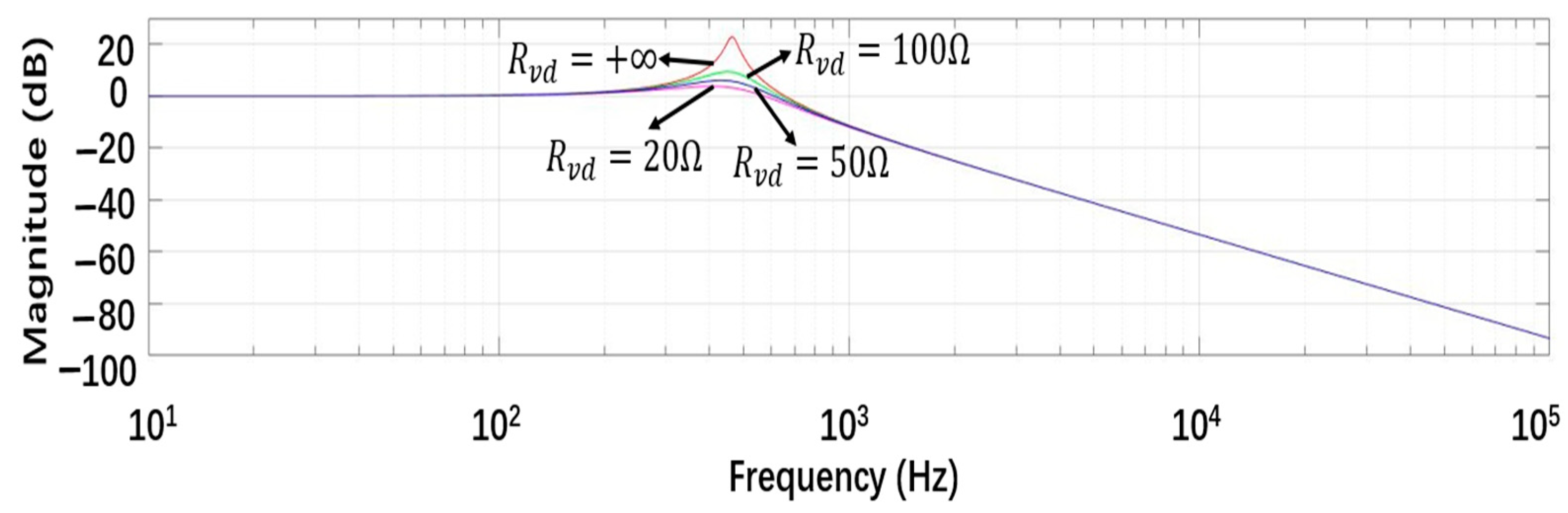
• A novel input filter resonance suppression (IFRS) method is proposed and applied in the VMMPCC for the TSMC, featuring good damping performance and easy implementation.

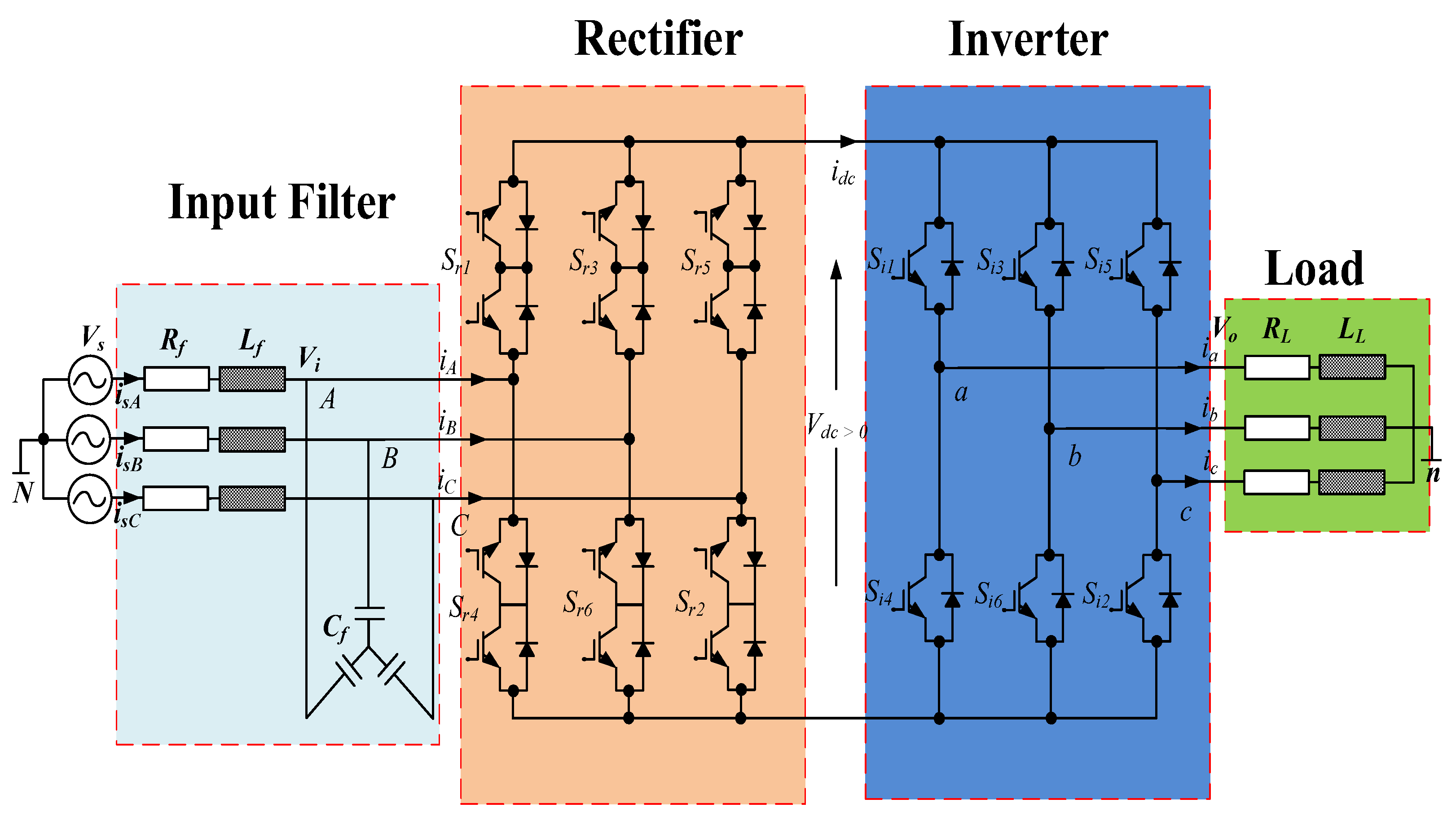
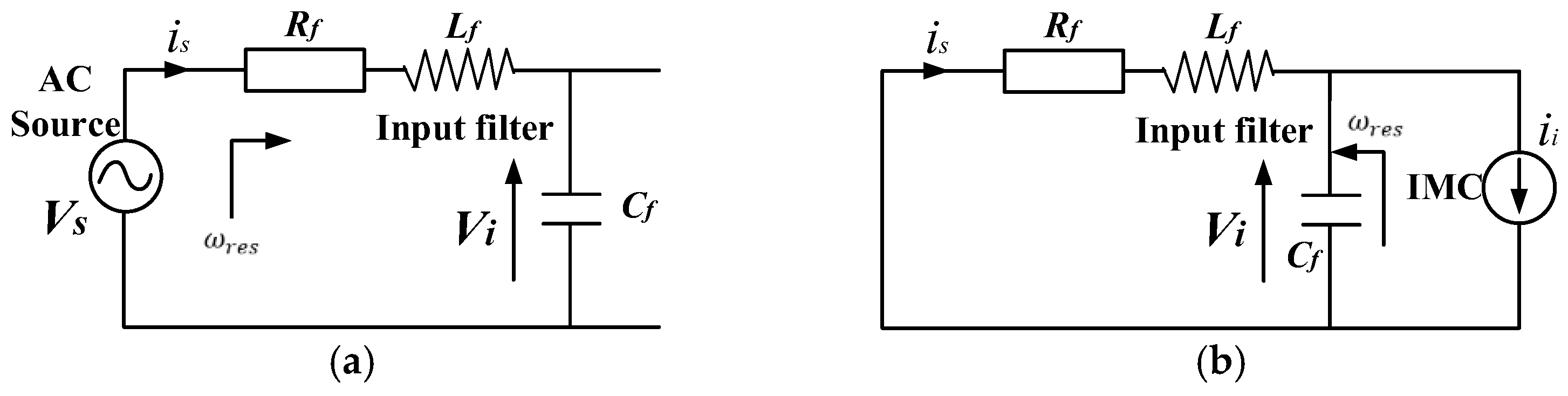
2. TSMC Mathematical System Model

The power circuit of the TSMC system is demonstrated in Figure 1. The TSMC is divided into the inverter stage and the rectifier stage.

For the rectifier stage, the relationship between $V_{dc}$ and $V_i$ is [2]:

$$V_{dc}=\left[\begin{array}{ccc}{S}_{r1}-S_{r4}& S_{r3}-S_{r6}& S_{r5}-S_{r2}\end{array}\right]V_i$$

(1)

$$S_{ri}=\{\begin{array}{c}0,\mathrm{open} \mathrm{state}\hfill \\ 1,\mathrm{closed} \mathrm{state}\hfill \end{array}$$

(2)

where $S_{ri}\left\{i\in \left(1,2,3,4,5,6\right)\right\}$ are the rectifier switching functions. In addition, the relationship between the input currents $i_i$ and the dc-link current $i_{dc}$ is [2]:

$$i_i=\left[\begin{array}{c}{S}_{r1}-S_{r4}\\ S_{r3}-S_{r6}\\ S_{r5}-S_{r2}\end{array}\right]i_{dc}$$

(3)

The relationship between $i_{dc}$ and $i_o$ for the inverter stage is:

$$i_{dc}=\left[\begin{array}{ccc}{S}_{i1}-S_{i4}& S_{i3}-S_{i6}& S_{i5}-S_{i2}\end{array}\right]i_o$$

(4)

$$S_{ix}=\{\begin{array}{c}0,\mathrm{open} \mathrm{state}\hfill \\ 1,\mathrm{closed} \mathrm{state}\hfill \end{array}$$

(5)

where $S_{ix}\left\{x\in \left(1,2,3,4,5,6\right)\right\}$ are the inverter switching functions. In addition, the relationship between the output voltage $V_o$ and the dc-link voltage $V_{dc}$ is [2]:

$$V_o=\left[\begin{array}{c}{S}_{i1}-S_{i4}\\ S_{i3}-S_{i6}\\ S_{i5}-S_{i2}\end{array}\right]V_{dc}$$

(6)

All the valid switching states are shown in

Table 2. Valid switching states of the rectifier.

${\mathit{V}}_{\mathit{d}\mathit{c}}$	${\mathit{i}}_{\mathit{A}}$	${\mathit{i}}_{\mathit{B}}$	${\mathit{i}}_{\mathit{C}}$	${\mathit{S}}_{\mathit{r}1}$	${\mathit{S}}_{\mathit{r}2}$	${\mathit{S}}_{\mathit{r}3}$	${\mathit{S}}_{\mathit{r}4}$	${\mathit{S}}_{\mathit{r}5}$	${\mathit{S}}_{\mathit{r}6}$
$V_{AC}$	$i_{dc}$	0	$-i_{dc}$	1	1	0	0	0	0
$V_{BC}$	0	$i_{dc}$	$-i_{dc}$	0	1	1	0	0	0
$-V_{AB}$	$-i_{dc}$	$i_{dc}$	0	0	0	1	1	0	0
$-V_{AC}$	$-i_{dc}$	0	$i_{dc}$	0	0	0	1	1	0
$-V_{BC}$	0	$-i_{dc}$	$i_{dc}$	0	0	0	0	1	1
$V_{AB}$	$i_{dc}$	$-i_{dc}$	0	1	0	0	0	0	1

and

Table 3. Valid switching states of the inverter.

${\mathit{i}}_{\mathit{d}\mathit{c}}$	${\mathit{V}}_{\mathit{a}\mathit{b}}$	${\mathit{V}}_{\mathit{b}\mathit{c}}$	${\mathit{V}}_{\mathit{c}\mathit{a}}$	${\mathit{S}}_{\mathit{i}1}$	${\mathit{S}}_{\mathit{i}2}$	${\mathit{S}}_{\mathit{i}3}$	${\mathit{S}}_{\mathit{i}4}$	${\mathit{S}}_{\mathit{i}5}$	${\mathit{S}}_{\mathit{i}6}$
$i_a$	$V_{dc}$	0	$-V_{dc}$	1	1	0	0	0	1
$i_a+i_b$	0	$V_{dc}$	$-V_{dc}$	1	1	1	0	0	0
$i_b$	$-V_{dc}$	$V_{dc}$	0	0	1	1	1	0	0
$i_b+i_c$	$-V_{dc}$	0	$V_{dc}$	0	0	1	1	1	0
$i_c$	0	$-V_{dc}$	$V_{dc}$	0	0	0	1	1	1
$i_a+i_c$	$V_{dc}$	$-V_{dc}$	0	1	0	0	0	1	1
0	0	0	0	1	0	1	0	1	0
0	0	0	0	0	1	0	1	0	1

.

In addition, an input filter is necessary to prevent over-voltages and harmonics and its model can be described as [2]:

$$\{\begin{array}{c}\frac{d{i}_s}{dt}=\frac{1}{L_f}\left(V_s-V_i\right)-\frac{R_f}{L_f}{i}_s\hfill \\ \frac{d{V}_i}{dt}=\frac{1}{C_f}\left(i_s-i_i\right)\hfill \end{array}$$

(7)

Similarly, the mathematical model in the load side is described as [2]:

$$V_o=L_L\frac{d{i}_o}{dt}+R_L{i}_o$$

(8)

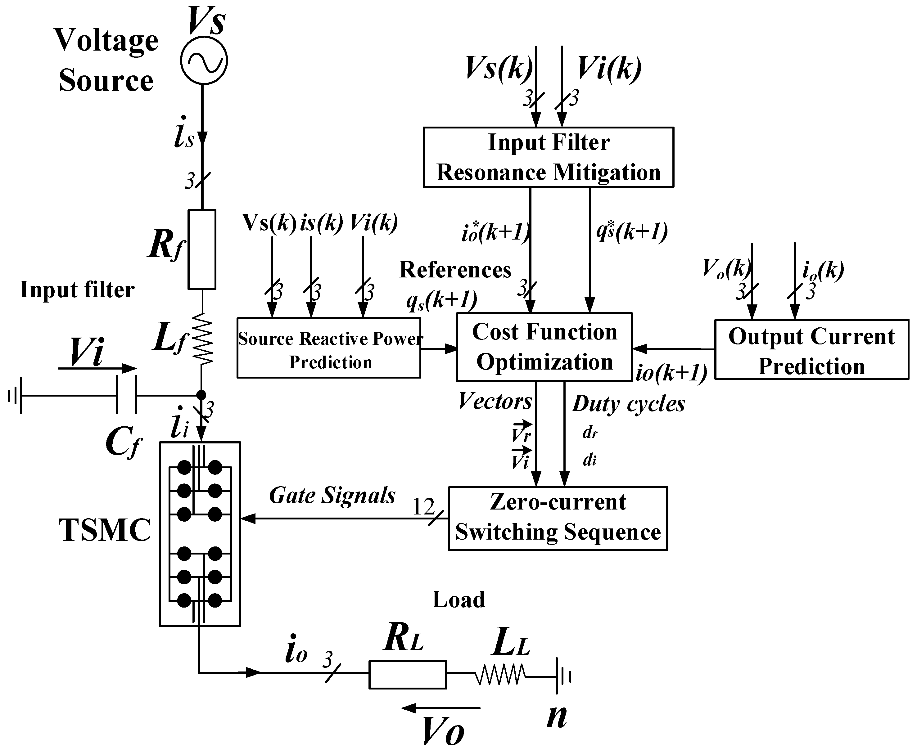
3. Vector Modulation Based Model Predictive Control Strategy with Zero-Current Switching Sequence

The block diagram of the VMMPCC with the ZSS and the IFRS for the TSMC system is shown in Figure 2, including output current prediction, source reactive power prediction, cost function, the IFRS and the ZSS.

Firstly, the IFRS generates the modified source reactive power reference $q_s^{*}\left(k+1\right)$ and output-current reference $i_o^{*}\left(k+1\right)$, then the output current prediction and the source reactive power prediction calculate $i_o\left(k+1\right)$, $q_s\left(k+1\right)$, which are the predicted values in the (k + 1)^th sampling period.

Secondly, with $i_o^{*}\left(k+1\right)$ and $q_s^{*}\left(k+1\right)$, the cost function selects the optimal switching states, which tracks their references at the end of the (k + 1)^th sampling instant.

Finally, in order to ensure safe zero-current switching operations, the proposed control strategy employs the ZSS scheme, in which the vectors are arranged in a symmetrical manner. The proposed control strategy is introduced in the following subsections.

3.1. Source Reactive Power Prediction and Output Current Prediction

The discrete model of input filter is [7,8]:

$$\begin{array}{c}\left[\begin{array}{c}{i}_s\left(k+1\right)\\ V_i\left(k+1\right)\end{array}\right]={\mathsf{\Phi }}_i\left[\begin{array}{c}{i}_s\left(k\right)\\ V_i\left(k\right)\end{array}\right]+{\mathsf{\Gamma }}_i\left[\begin{array}{c}{V}_s\left(k\right)\\ i_i\left(k\right)\end{array}\right]\\ A_i=\left[\begin{array}{cc}-R_f/L_f& -1/L_f\\ 1/C_f& 0\end{array}\right],B_i=\left[\begin{array}{cc}1/L_f& 0\\ 0& -1/C_f\end{array}\right]\end{array}$$

(9)

where ${\mathsf{\Phi }}_i=e^{A_i{T}_s},{\mathsf{\Gamma }}_i=A_i^{-1}\left({\mathsf{\Phi }}_i-I\right)B_i$, $R_f,$ $L_f$ and $C_f$ are the parameters of the input filter, $T_s$ is the sampling time.

$q_s\left(k+1\right)$ can be expressed as:

$$q_s\left(k+1\right)=v_{s\alpha }\left(k+1\right)i_{s\beta }\left(k+1\right)-v_{s\beta }\left(k+1\right)i_{s\alpha }\left(k+1\right)$$

(10)

where $i_{s\alpha }\left(k+1\right),i_{s\beta }\left(k+1\right)$ are the predicted source current and $v_{s\alpha }\left(k+1\right),v_{s\beta }\left(k+1\right)$ represent the source voltage in the (k+1)^th sampling period in $\alpha \beta$ reference frame.

Similarly, for the load stage, the discrete state-space model is calculated as [7,8]:

$$i_o\left(k+1\right)={\Phi }_o{i}_o\left(k\right)+{\Gamma }_o{V}_o\left(k\right)$$

(11)

where $L_L$ and $R_L$ are the load inductance and resistance,${\Phi }_o=e^{-\frac{R_L}{L_L}{T}_s}$, ${\Gamma }_o=-\frac{1}{R_L}({\Phi }_o-1$).

3.2. Cost Function Optimization

For the inverter stage, six active vectors and two zero vectors are valid as shown in Figure 3a and associated with switching states in Table 3. The VMMPCC strategy uses two adjacent vectors $V_{i1},V_{i2}$ and one zero vector $V_{i0}$.

Since the fundamental frequency is much lower than the sampling frequency and, thus, the control objective $e_i$ error can be approximated as [18]:

$$e_i=\left\{d_{ij}{e}_{ij}\right\}$$

(12)

where $e_{ij}$ represents the error when only vector $V_{ij}\left\{j\in \left(0,1,2\right)\right\}$ is applied for the whole sampling period $T_s$ and $d_{ij}$ is the duty cycle of $V_{ij}$.

Define $e_{iRMS}$ as the root mean square (RMS) value of all the weighted errors, which can be calculated as [18]:

$$e_{iRMS}=\sqrt{\frac{{\sum }_{j=0}^2{(d_{ij}{e}_{ij})}^2}{3}}$$

(13)

and the mean value of the weighted errors is defined as [18]:

$$\overline{e_i}=\frac{1}{3}\sum _{j=0}^2\left(d_{ij}{e}_{ij}\right)$$

(14)

Since that $d_{ij}{e}_{ij}\ge 0$, minimizing $e_i$ yields minimum values of $\overline{e_i}$ and $e_{iRMS}$. On this basis, the duty cycles can be obtained based on minimizing (13) as

$$mi{n}_{d_i}{G}_i=\frac{1}{3}\sum _{j=0}^2{(d_{ij}{e}_{ij})}^2=\frac{1}{3}\sum _{j=0}^2{g}_{ij}{\left(d_{ij}\right)}^2$$

(15)

$$\sum _{j=0}^2{d}_{ij}=1,\left(0\le d_{ij}\le 1\right)$$

(16)

This optimization problem could be solved using the Lagrange multipliers method. To find the stationary points of a function $f\left(x,y\right)$ subject to the constraint $g\left(x,y\right)=0$, the Lagrangian function is defined as [23]:

$$L\left(x,y,\lambda \right)=f\left(x,y\right)+\lambda g\left(x,y\right)$$

(17)

Then, the optimization problem turns to minimization of (18):

$$f\left(d_{i0},d_{i1},d_{i2}\right)=\frac{1}{3}{g}_0{d}_{i0}^2+\frac{1}{3}{g}_1{d}_{i1}^2+\frac{1}{3}{g}_2{d}_{i2}^2$$

(18)

$$g_i={\left(i_o^{*}\left(k+1\right)-i_o\left(k+1\right)\right)}^2$$

(19)

In (18), $d_{i0},d_{i1},d_{i2}$ are the duty cycles and $g_0,g_1,g_2$ represent the cost function values for three active vectors $V_{i0},V_{i1},V_{i2}$. The constraint is

$$g\left(d_{i0},d_{i1},d_{i2}\right)=d_{i0}+d_{i1}+d_{i2}-1$$

(20)

Rewrite the Lagrangian function by substituting (18) and (20) into (17) as

$$L\left(d_{i0},d_{i1},d_{i2},\lambda \right)=\frac{1}{3}{g}_0{d}_{i0}^2+\frac{1}{3}{g}_1{d}_{i1}^2+\frac{1}{3}{g}_2{d}_{i2}^2+\lambda \left(d_{i0}+d_{i1}+d_{i2}-1\right)$$

(21)

Then, the gradient of $L\left(d_{i0},d_{i1},d_{i2},\lambda \right)$ can be obtained as

$${\nabla }_{d_{i0},d_{i1},d_{i2},\lambda }L\left(d_{i0},d_{i1},d_{i2},\lambda \right)=\left(\frac{\partial L}{\partial d_{i0}},\frac{\partial L}{\partial d_{i1}},\frac{\partial L}{\partial d_{i2}},\frac{\partial L}{\partial \lambda }\right)$$

(22)

Substitute (21) into (22)

$${\nabla }_{d_{i0},d_{i1},d_{i2},\lambda }L\left(d_{i0},d_{i1},d_{i2},\lambda \right)=\left(\frac{2}{3}{g}_0{d}_{i0}+\lambda ,\frac{2}{3}{g}_1{d}_{i1}+\lambda ,\frac{2}{3}{g}_2{d}_{i2}+\lambda ,d_{i0}+d_{i1}+d_{i2}-1\right)$$

(23)

Consider the minimization condition

$${\nabla }_{d_{i0},d_{i1},d_{i2},\lambda }L\left(d_{i0},d_{i1},d_{i2},\lambda \right)=0$$

(24)

Combine (23) and (24), the duty cycles can be obtained as

$$\{\begin{array}{c}{d}_{i0}=\frac{g_1{g}_2}{g_0{g}_1+g_0{g}_2+g_1{g}_2}\\ d_{i1}=\frac{g_0{g}_2}{g_0{g}_1+g_0{g}_2+g_1{g}_2}\\ d_{i2}=\frac{g_0{g}_1}{g_0{g}_1+g_0{g}_2+g_1{g}_2}\end{array}$$

(25)

$$\lambda =-\frac{2}{3}\frac{g_0{g}_1{g}_2}{g_0{g}_1+g_0{g}_2+g_1{g}_2}$$

(26)

The total cost function $g_i$ and the synthesized vector $V_{is}$ can be expressed as follows:

$$g_i=d_{i0}{g}_{i0+}{d}_{i1}{g}_{i1}+d_{i2}{g}_{i2}$$

(27)

$$V_{is}=d_{i0}{V}_{i0+}{d}_{i1}{V}_{i1}+d_{i2}{V}_{i2}$$

(28)

In the similar way, six active vectors for the rectifier stage are considered as shown in Figure 3b, associated with switching states in Table 2. The VMMPCC strategy considers two valid adjacent vectors $V_{r1},V_{r2}$ and assesses two respective cost functions $g_{r1},g_{r2}$. The duty cycles $d_{r1},d_{r2}$ can be calculated as:

$$\{\begin{array}{c}{d}_{r1}=g_{r2}/\left(g_{r1}+g_{r2}\right)\hfill \\ d_{r2}=g_{r1}/\left(g_{r1}+g_{r2}\right)\hfill \\ d_{r1}+d_{r2}=1\hfill \end{array}$$

(29)

$$g_r={\left(q_s^{*}-q_s\left(k+1\right)\right)}^2$$

(30)

with $d_{r1},d_{r2}$, the total cost function $g_r$ and the synthesized vector $V_{rs}$ can be expressed as:

$$g_r=d_{r1}{g}_{r1}+d_{r2}{g}_{r2}$$

(31)

$$V_{rs}=d_{r1}{V}_{r1}+d_{r2}{V}_{r2}$$

(32)

3.3. Comparision between the Proposed VMMPCC and the CMPC

As shown in Figure 3b, the length of the segment NQ is $g_{r1}$, defined as the error when only the vector $V_{r1}$ is applied and the length of the segment MN is $g_{r2}$, defined as the error when only the vector $V_{r2}$ is applied, respectively.

From Equations (29)–(34) can be obtained:

$$V_{rs}=V_{r2}+d_{r1}\left(V_{r1}-V_{r2}\right)$$

(33)

$$V_{rs}=V_{r1}+d_{r2}\left(V_{r2}-V_{r1}\right)$$

(34)

From Equations (33) and (34), obviously that the end point of $V_{rs}$ (tagged as P) should be located on MQ and the length of MQ is $d_{MQ}$. In addition, the length of the segment MP is $d_{r1}{d}_{MQ}$ and the length of MP is $d_{r2}{d}_{MQ}$, respectively.

Consider Equations (29), (33) and (34) and the law of sines, (35) can be obtained:

$$\frac{\sin \left(\angle \mathrm{MNP}\right)}{\sin \left(\angle \mathrm{MPN}\right)}=\frac{d_{r1}{d}_{MQ}}{g_{\mathrm{r}2}}=\frac{d_{r2}{d}_{MQ}}{g_{\mathrm{r}1}}=\frac{\sin \left(\angle \mathrm{PNQ}\right)}{\sin \left(\angle \mathrm{NPQ}\right)}$$

(35)

Besides, since $\angle \mathrm{MPN}+\angle \mathrm{NPQ}=\mathsf{\pi }$, thus, $\sin \left(\angle \mathrm{MPN}\right)=\sin \left(\angle \mathrm{NPQ}\right)$, (36) can be obtained as:

$$\sin \left(\angle \mathrm{MNP}\right)=\sin \left(\angle \mathrm{PNQ}\right)$$

(36)

Consider two conditions based on (36):

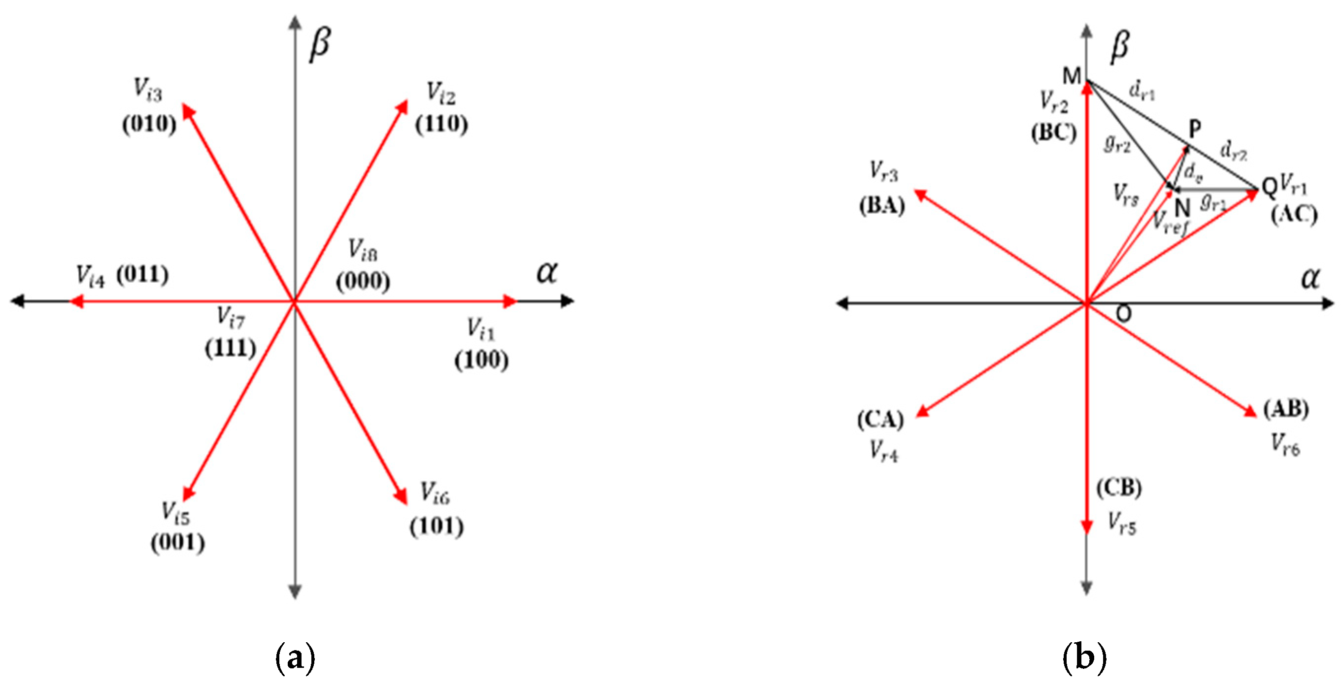
• $\angle \mathrm{MNP}+\angle \mathrm{PNQ}=\mathsf{\pi }$; This means that P and Q are the same points and the error $d_e$ between the synthesized vector $V_{rs}$ and the reference vector $V_{ref}$ (equal to the length of PN) is zero;
• $\angle \mathrm{MNP}=\angle \mathrm{PNQ}.$ In fact, since:

  $$\{\begin{array}{c}\angle \mathrm{NQP}<\angle \mathrm{OQM} =\mathsf{\pi }/3\hfill \\ \angle \mathrm{NPQ}=\angle \mathrm{MNP}+\angle \mathrm{NMP}>\angle \mathrm{PNQ}\hfill \\ \angle \mathrm{PNQ}+\angle \mathrm{NPQ}=\mathsf{\pi }-\angle \mathrm{NQP}>2\mathsf{\pi }/3\hfill \end{array}$$

  (37)

Thus, $\angle \mathrm{NPQ}>\mathsf{\pi }/3>\angle \mathrm{NQP}$. $d_e<g_{r1 }$ is obtained based on the law of sine. In the similar way,$d_e<g_{r2}$ is deduced. Both the two conditions verify the advantages of the VMMPCC strategy over the CMPC.

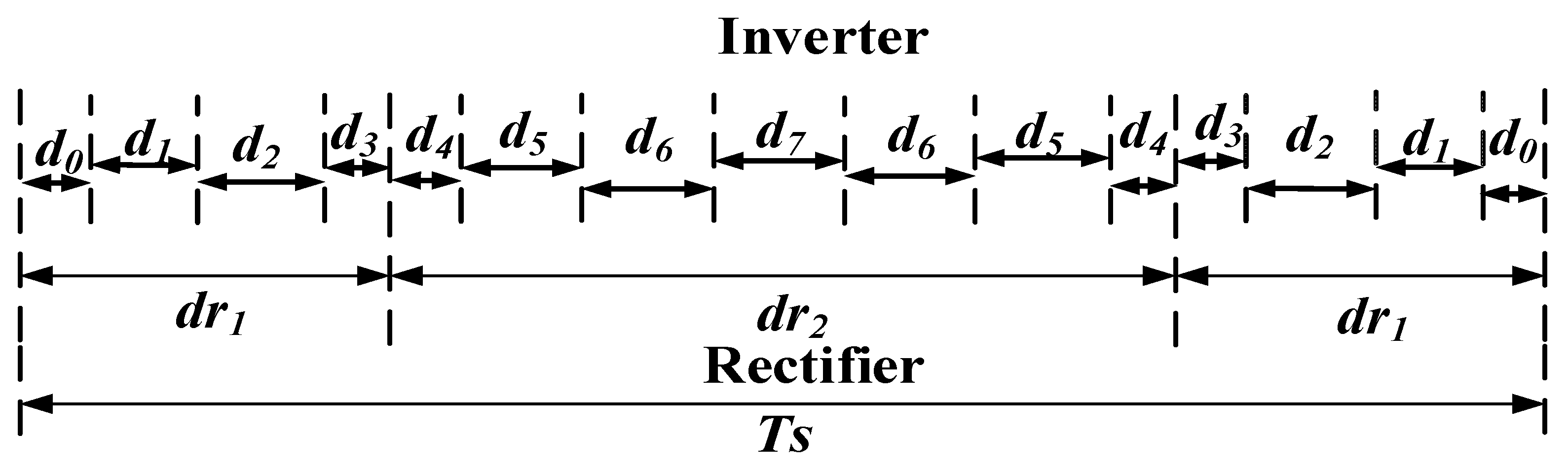
3.4. Zero-Current Switching Sequence

As can be seen in Figure 1, the rectifier stage connects the inverter stage directly. A zero-current switching sequence is proposed in this paper. The ZSS proposed is shown in Figure 4.

The duty cycles $d_0~d_7$ for the inverter are calculated as:

$$\{\begin{array}{c}{d}_0=d_3=\frac{d_{i1}{d}_{i0}}{4}\hfill \\ d_1=\frac{d_{i1}{d}_{r1}}{2}\hfill \\ d_2=\frac{d_{i2}{d}_{r1}}{2}\hfill \\ d_4=\frac{d_{i2}{d}_{i0}}{4}\hfill \\ d_5=\frac{d_{i2}{d}_{r2}}{2}\hfill \\ d_6=\frac{d_{i1}{d}_{r2}}{2}\hfill \\ d_7=\frac{d_{i2}{d}_{i0}}{2}\hfill \end{array}$$

(38)

Moreover, the duty cycles $d_{r1}~d_{r2}$ for the rectifier are

$$\{\begin{array}{c}{d}_{r1}=2d_0+d_1+d_2\hfill \\ d_{r2}=2\left(d_4+d_5+d_6\right)+d_7\hfill \end{array}$$

(39)

Obviously, the rectifier state commutation always happens, when zero voltage vector is implemented for the inverter and $i_{dc}=0$. Owing to this, zero-current switching operations and reduction of the switching losses of the TSMC are achieved, which can simplify the commutation strategy.

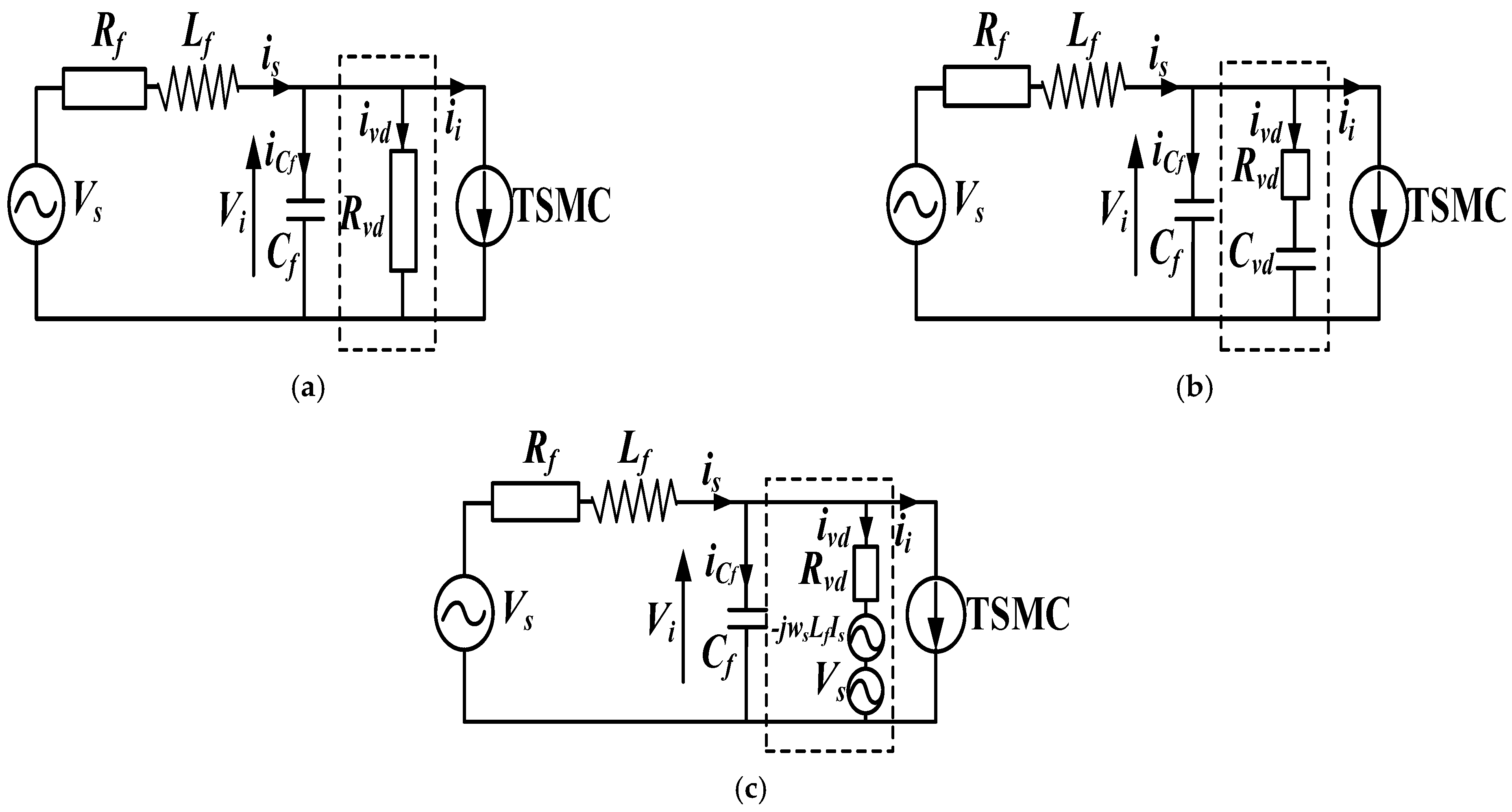
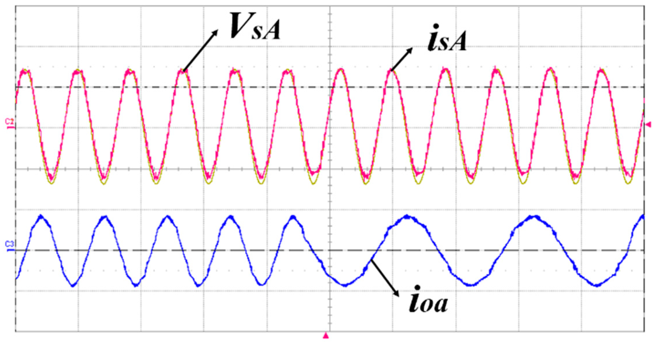
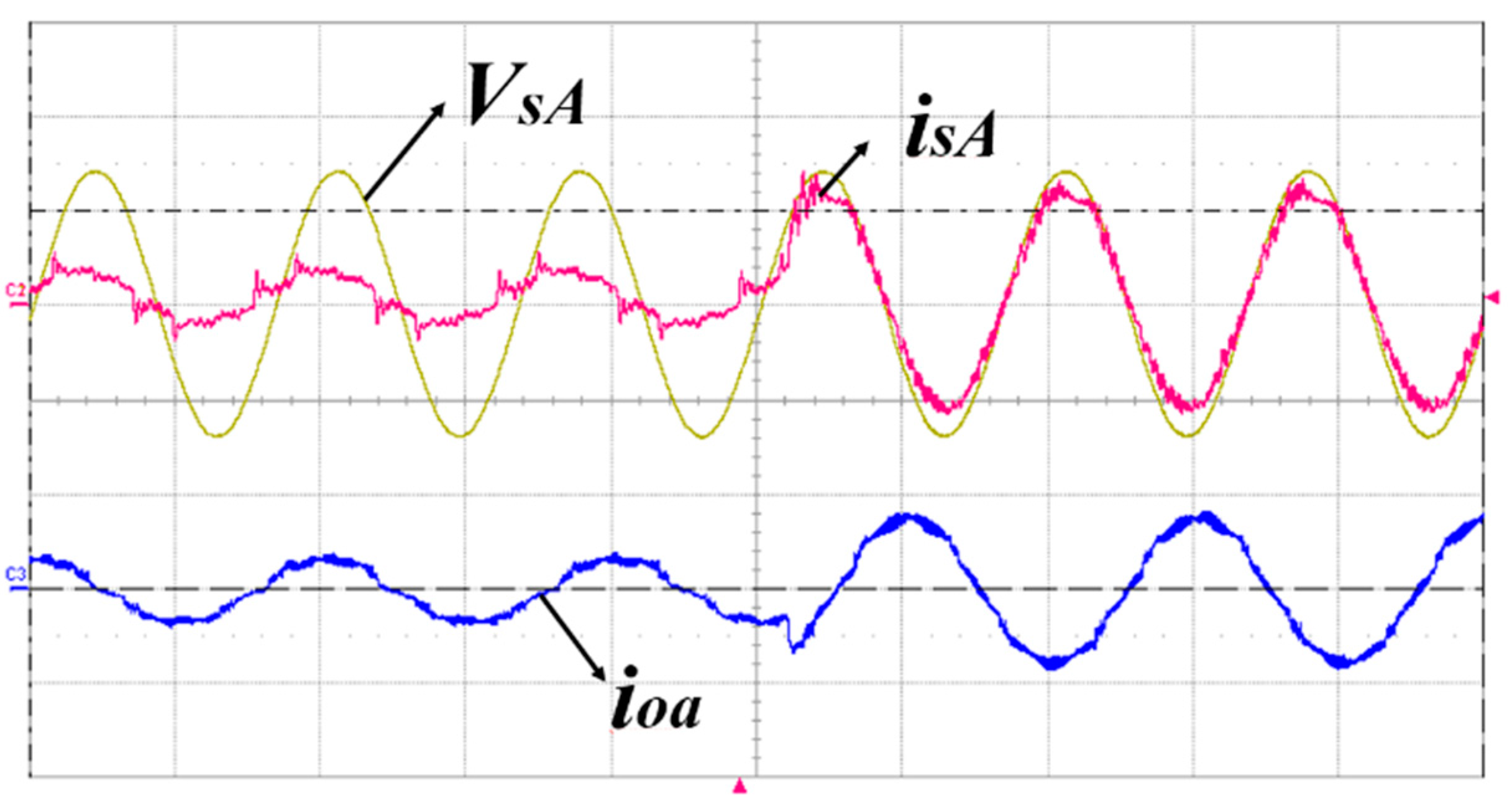
4. Input Filter Resonance Suppression

An active damping technique is crucial to the TSMC control system [26,27,28,29,30,31,32,33], as shown in Figure 5. Figure 5a shows the traditional active damping method 1 [26,27,28,29,30], which considers a virtual resistor $R_{vd}$ placed in parallel with $C_f$. Figure 5b shows another active damping method 2 [31,32,33], the virtual branch is considered in parallel with $C_f$, consisting of a virtual resistor $R_{vd}$ in series with a virtual capacitor $C_{vd}$. The main drawback of method 1 and method 2 is the limited effectiveness and applications. From Figure 5a,b, the damping current $i_{vd}$ is obtained from the input voltage $V_i$, which contains fundamental frequency components and will affect the normal operations of the TSMC. In [31,32,33], dc blockers are stilled applied to filter the capacitor voltages, even when the source voltages and source currents are also available. The digital filters worsen the dynamic performance and even could limit the range of parameters adjustment. Figure 5c shows the proposed active damping method, the virtual branch consists of a virtual damping resistor $R_{vd}$, a virtual voltage source same as the source voltage $V_s$ and an added item $\mathrm{j}{\omega }_s{L}_f{I}_s$, where ${\omega }_s$ denotes the source frequency and $I_s$ represents the fundamental source current under steady state. $I_s$ can be obtained based on instantaneous power theory [34].

$$I_s=\left(P_i^{*}+j{Q}_i^{*}\right)V_s/\Vert V_s\Vert {}^2$$

(40)

and the damping current $i_{vd}$ is expressed as:

$$i_{vd}=\frac{V_i-V_s+\mathrm{sj}{\omega }_s{L}_f{I}_s}{R_{vd}}$$

(41)

In (41), the items $V_s$ and s$\mathrm{j}{\omega }_s{L}_f{I}_s$ contribute to remove the fundamental frequency component in $i_{vd}$, in such way $i_{vd}$ will not affect the control accuracy and improve the effectiveness of active damping.

The small-signal transfer function from $i_i$ to $i_s$ can be expressed as:

$$\mathrm{G}\left(\mathrm{s}\right)=\frac{1}{s^2{L}_f{C}_f+s\left(L_f/R_{vd}+\left(1+R_f/R_{vd}\right)C_f\right)+1+R_f/R_{vd}}$$

(42)

From Figure 6, it is obvious that when $R_{vd}$ decreases, the damping coefficient increases. Meanwhile, the magnitude at high frequency does not change, which means the proposed IFRS method can achieve both good filtering and damping performance.

As shown in Figure 5c, the source current $i_s$ is expressed as:

$$i_s=i_i+i_{C_f}+i_{vd}$$

(43)

Thus, the damping effect can be realized by modifying the reference value of $i_s$ by injecting $i_{vd}$. However, rather than the source current $i_s$, the proposed VMMPCC strategy controls source reactive power and output currents directly (seen in Equations (19) and (30)). Hence, the input apparent power $s_i$ can be obtained as:

$$s_i=V_i{i}_s^C=V_i\left(i_i^C+i_{C_f}^C\right)+V_i{i}_{vd}^C$$

(44)

From (44), the damping effect can be realized by injecting $V_i{i}_{vd}^C$ into the reference values of $s_i$. Therefore, the reference value of input active power $p_i$ should be modified with the real part of $V_i{i}_{vd}^C$ and the reference value of reactive power $q_i$ should be modified with the imaginary part of $V_i{i}_{vd}^C$, respectively,

$$p_i^{*}=P_i^{*}+Re\left(V_i{i}_{vd}^c\right)$$

(45)

$$q_i^{*}=Q_i^{*}+Im\left(V_i{i}_{vd}^c\right)$$

(46)

It should be noticed here, in this paper, that rather than the input active power $p_i$, the proposed VMMPCC strategy controls output currents directly. Thus, (45) cannot be applied directly. The relationship between the input active power $p_i$ and output active power $p_L$ is [12]:

$$p_i^{*}\eta =p_L^{*}=\frac{3}{2}{R}_L{\left(I_o^{*}\right)}^2$$

(47)

where $\eta$ represents the efficiency of the TSMC and $I_o^{*}$ is the reference amplitude of output currents.

Thus, the reference amplitude of output currents $i_o^{*}$ can be modified as shown in (48):

$$i_o^{*}=\sqrt{{\left(I_o^{*}\right)}^2+\frac{2\eta Re\left(V_i{i}_{vd}^c\right)}{3R_L}}$$

(48)

In addition, the source reactive power $q_s$ can be obtained as:

$$\begin{array}{cc}{q}_s=Im\left(V_s{i}_s^c\right)\hfill & =Im\left[\left(V_i+R_f{i}_s+L_f\frac{d{i}_s}{dt}\right)i_s^c\right]=Im\left(V_i{i}_s^c+L_f\frac{d{i}_s}{dt}{i}_s^c\right)\\ & =q_i+L_f\frac{d{i}_s}{dt}{i}_s^c\hfill \end{array}$$

(49)

From Equation (49), it is obvious that the difference between $q_s$ and $q_i$ is related to the voltage drop on $L_f$, which is negligible compared with $V_s$ in a proper LC filter. Hence, $q_i$ and $q_s$ can be considered equal.

Finally, the IFRS is implemented by modifying the reference values $i_o^{*}$ with the real part of $V_i{i}_{vd}^c$ and $q_s^{*}$ with the imaginary part of $V_i{i}_{vd}^c$.

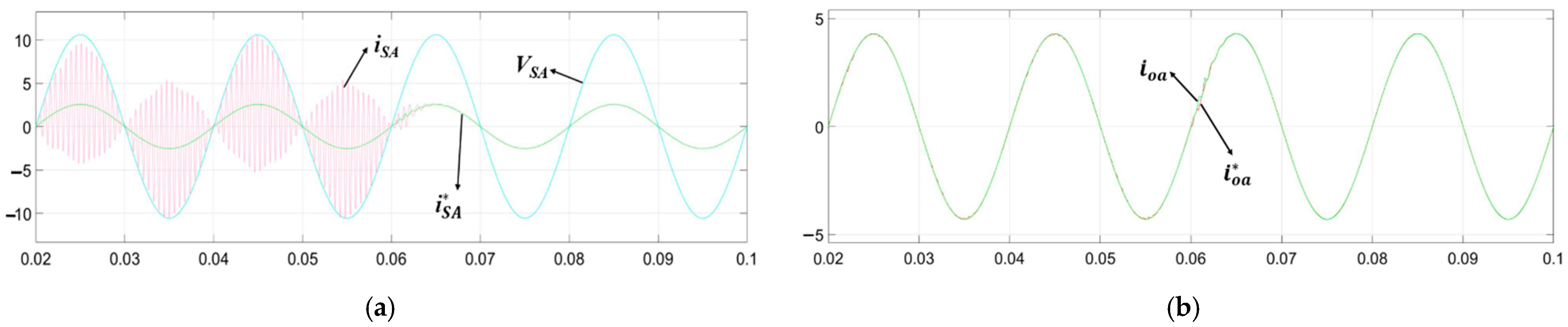
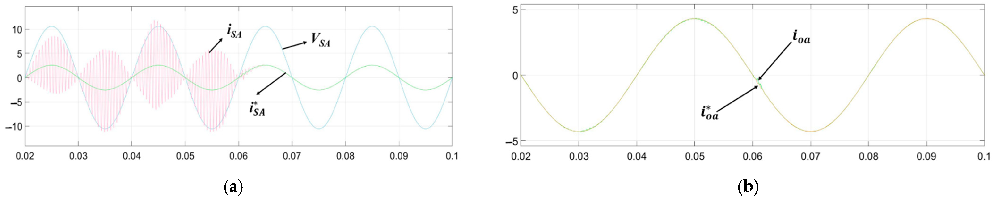
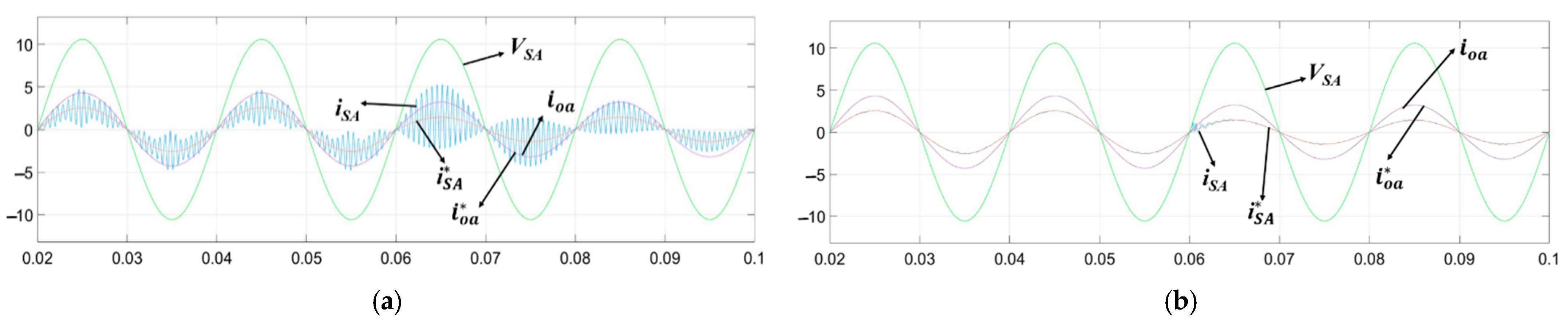
5. Simulation Results

To verify the proposed strategy, simulation has been done and the relevant parameters are demonstrated in

Table 4. System parameters.

$V_s$	The amplitude of source voltage	141 V
$L_f$	Input filter inductor	5 mH
$R_f$	Input filter resistor	0.5$\mathsf{\Omega }$
$C_f$	Input filter capacitor	21 μF
$L_L$	Load inductor	5 mH
$R_L$	Load resistor	5$\mathsf{\Omega }$
$T_s$	Sampling time	100 μs
$f_s$	Sampling frequency	10 kHz

.

The input filter resonance can be excited by the utility (series resonance) due to the potential fifth and seventh harmonics in the AC source (seen in Figure 7a) and also by the converter itself (parallel resonance seen in Figure 7b). Normally, the filter resonant frequency is designed both one decade above the input supply frequency $f_w$ and one decade below the switching frequency $f_s$ to minimize the effect of the resonance introduced by the filter [35]. That is

$$10f_w<f_{res}=\frac{1}{2\pi \sqrt{LC}}<10f_s$$

(50)

In this paper, the resonant frequency is designed and situated nearly at the seventh harmonic of the source system to excite the resonant situation, in which the TSMC system performance can be compared with the IFRS and without the IFRS [35].

$$f_{res}=\frac{1}{2\pi \sqrt{LC}}\approx 7\left(\mathrm{pu}\right)$$

(51)

As shown in Figure 8, the IFRS is added at 0.06 s. Before that, the source current is highly distorted due to the input filter resonance. After 0.06 s, obviously the source current is significantly improved and achieves a very good tracking to its reference. Besides, the output current shows an almost sinusoidal waveform and approaches its reference in Figure 8b. The results of another simulation group are shown in Figure 9, where the reference of the output-current frequency is changed to 25 Hz. As shown in Figure 8 and Figure 9, the IFRS can greatly improve the quality of source current in spite of system reference variations. In addition, the source reactive power is minimized based on the Equations (10) and (30).

In order to verify the dynamic performance of the proposed VMMPCC strategy for the TSMC, two groups of simulation are implemented and the results are shown in Figure 10 and Figure 11, considering the two conditions of with the IFRS and without the IFRS. In Figure 10, the output-current frequency steps from 25 Hz to 50 Hz. In Figure 11, the output-current reference amplitude steps from 4 A to 2 A. As shown in Figure 10b and Figure 11b, the system resumes quickly after minute oscillations in a short time, when the output-current frequency or the output-current reference amplitude steps at t = 0.06 s. Besides, the output current and the source current still present good sinusoidal waveforms with the IFRS and the source reactive power is minimized, when the reference of the output-current amplitude and the reference of output-current frequency steps. At last, the control scheme presents a good dynamic performance in both input and output sides.

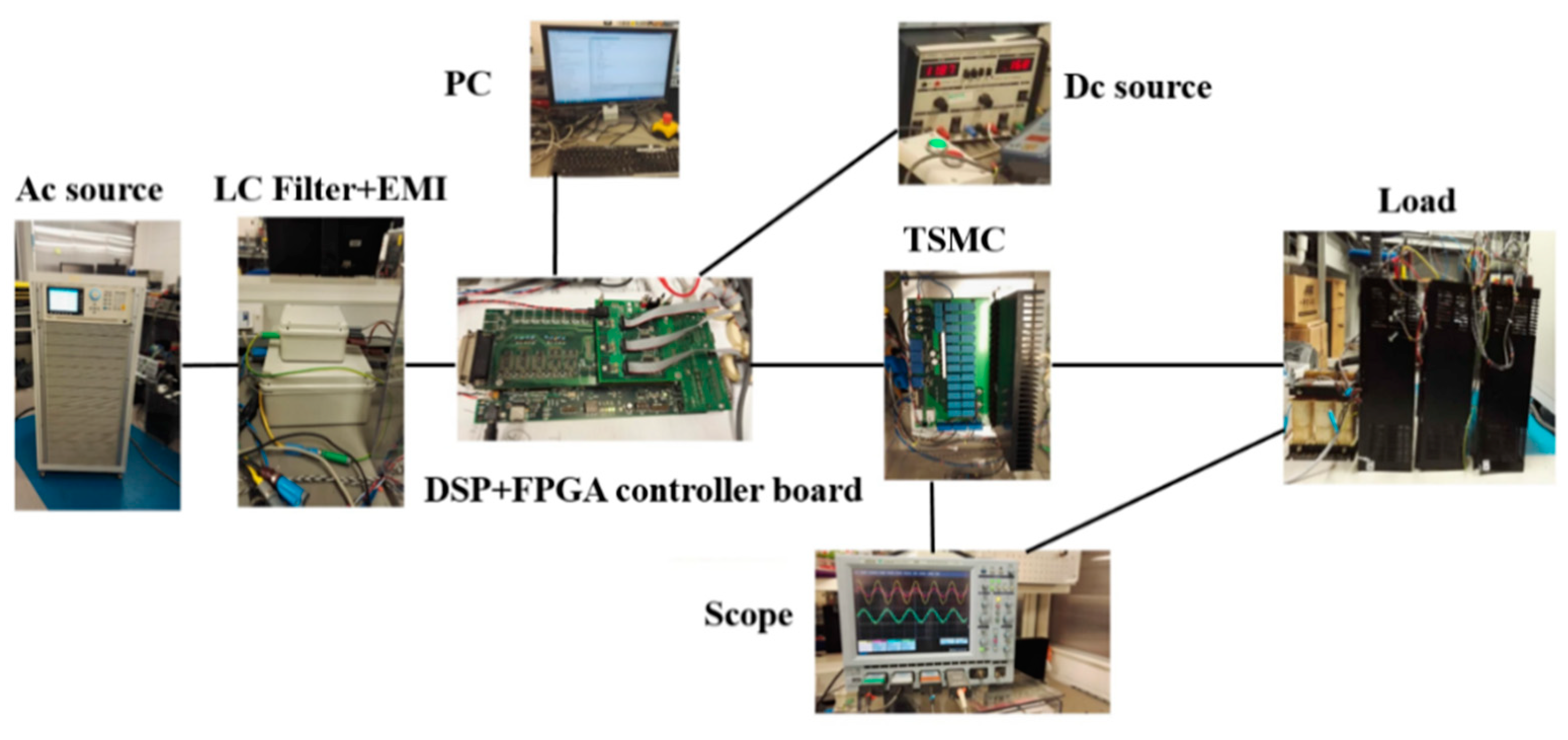
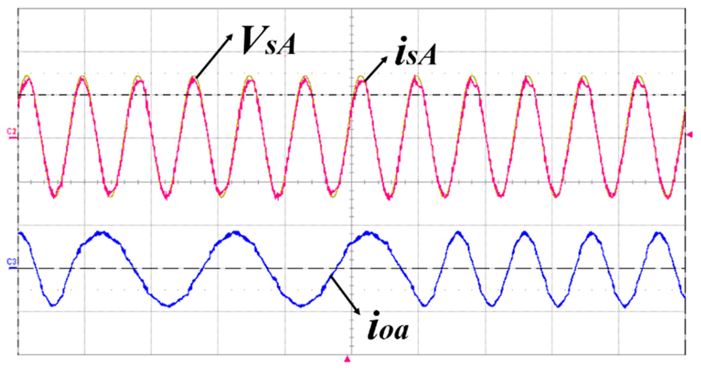
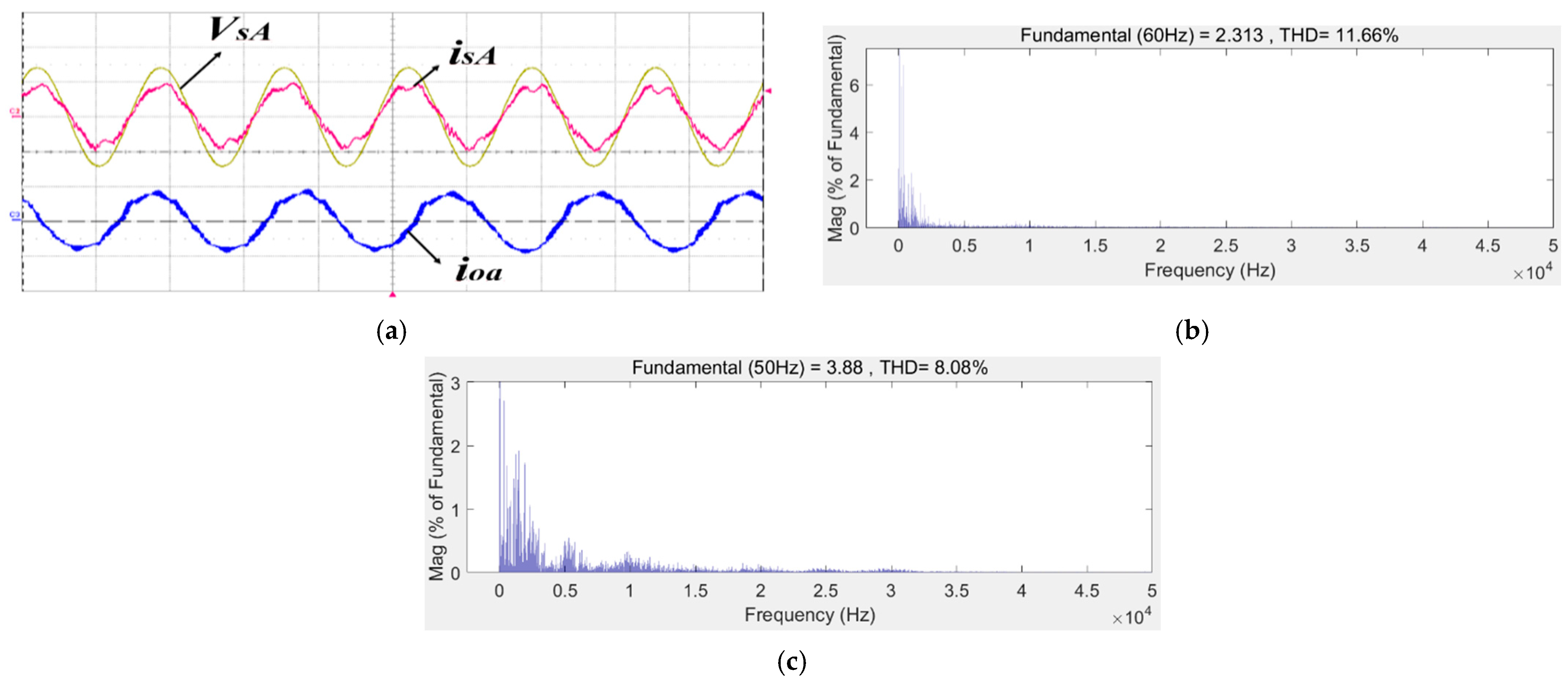
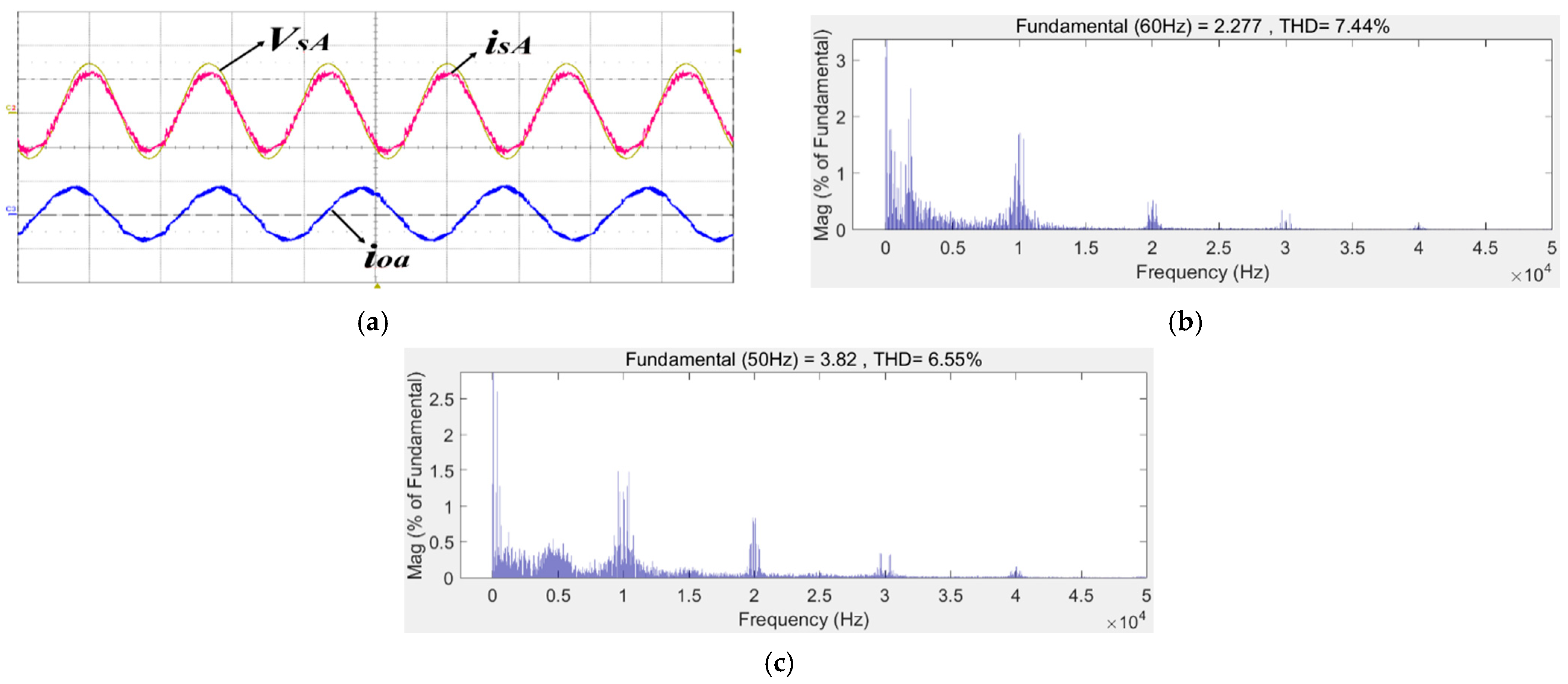
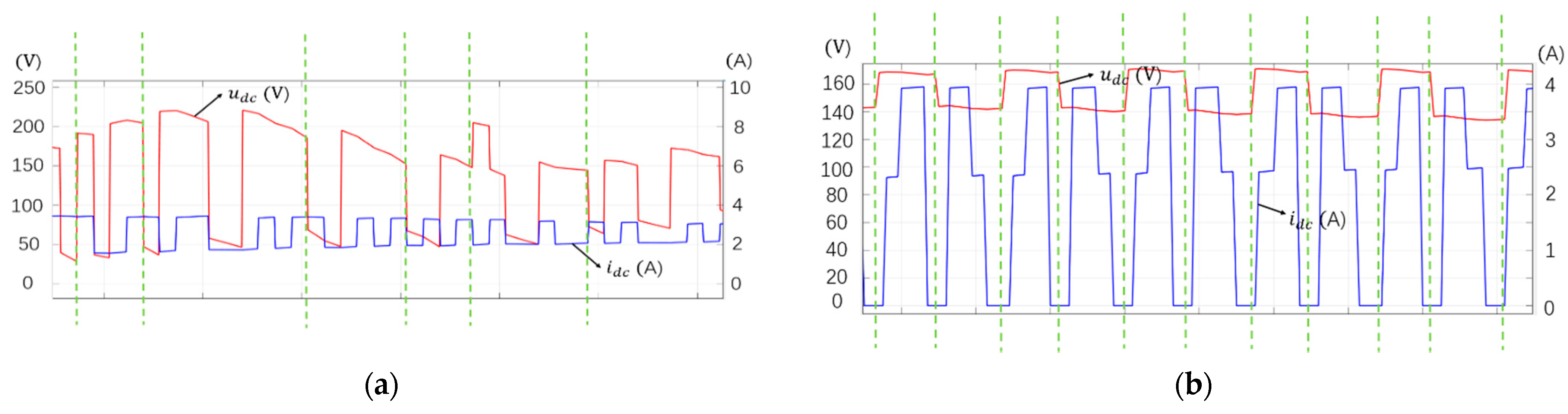
6. Experimental Results

To verify the proposed strategy, a laboratory prototype is designed and built for experimental evaluation. The prototype is shown in Figure 12 and the relevant experimental parameters are shown in Table 4. A digital control board integrating a ProASIC3 FPGA and a Texas Instruments C6713 DSP is used for the test and verification. Unlike the OSMC, where Silicon Carbide (SiC) MOSFETs are used for all the eighteen switches, this experiment use 12 standard insulated gate bipolar transistors (IGBT, IKW15T120) for the rectifier and six SiC MOSFETs (C2M0080120D) for the inverter, considering the high switching frequencies and the switching losses. In addition, a radiator is used to dissipate the heat produced by the high frequency switches. Moreover, the ac source output side connects an EMI filter, more details can be found in [36].

Figure 13 shows the results of the conventional model predictive control strategy for the TSMC without the IFRS and the ZSS. From Figure 13, $i_{sA}$ is highly distorted, mainly related to the input filter resonance. As seen in Figure 13b, the main distortions are situated around the input filter resonance frequency. Moreover, the waveforms of $V_{sA}$ and $i_{oa}$ are also affected by the large oscillations of $i_s$, due to the direct topology of the TSMC. From Figure 13, the input filter resonance is necessary to be suppressed to improve the power-quality performance of the TSMC system.

Figure 14 demonstrates the results of the situation, where the IFRS is added to the CMPC for the TSMC. Compared with Figure 13, with the help of the IFRS, the quality of $i_{sA}$ is largely improved and the THD of the output current is also improved from 10.16% to 8.08% respectively. In addition, the variable switching frequency phenomenon can be easily observed in Figure 14b,c. In addition, $i_{sA}$ is not always in phase with $V_{sA}$ in Figure 14a, which indicates that the minimization of the instantaneous source reactive power based on Equations (10) and (30) need to be improved.

Figure 15 shows the results of the proposed VMMPCC strategy with the IFRS and the ZSS. Compared with Figure 14a, the source current $i_{sA}$ is improved with a THD from 11.66% to 7.44% and the THD of the output current is also improved from 8.08% to 6.55% respectively. In addition, the fixed switching frequency phenomenon can be easily observed in Figure 15b,c. In addition, $i_{sA}$ is always in phase with $V_{sA}$ in Figure 15a, which indicates the minimization of the instantaneous source reactive power based on Equations (10) and (30) is also improved compared with Figure 14a.

The instantaneous source reactive power is controlled in the proposed control strategy in the input side, thus, the parameter named as the mean power $M_p$ is defined to assess the performance [7]:

$$M_p=\frac{1}{m}\sum _{k=1}^m\left|p\left(k\right)\right|$$

(52)

In Equation (52), m is set to 10,000 and $p\left(k\right)$ is the actual value of power at the k^th sampling instant.

The comparisons between the CMPC and the proposed VMMPCC with the ZSS are shown in

Table 5. The assessment parameters of experimental results.

Method	${\mathit{M}}_{ {\mathit{q}}_{\mathit{s}}}\left(\mathbf{Var}\right)$	$\mathbf{THD}\mathbf{of}{\mathit{i}}_{\mathit{s}}$	$\mathbf{THD}\mathbf{of}{\mathit{i}}_{\mathit{a}}$
CMPC	9.37	11.66%	8.08%
VMMPCC	2.49	7.44%	6.55%

.

As shown in Table 5, the proposed VMMPCC with the ZSS can obtain better performance in all aspects of the instantaneous source reactive power, the source current and the output current, compared with the CMPC.

The CMPC may obtain the similar performance with the VMMPCC in aspects of control objectives, by using a much higher sampling frequency than that in the VMMPCC [18,24]. In fact, predictive controllers usually occupy the computational resources and, thus, the sampling frequency cannot always be increased in practical applications. In addition, the variable switching frequency with the CMPC is a lurking peril for the control system [31].

Besides, the amplitude of the output current is 3.82 A; thus, there exists a 4.5% steady state error, because that the reference of the output current is set to 4A. In fact, a steady state error between the measured current and its reference is normal in model-based control strategies, where a steady-state error usually occurs from the system model inaccuracies. This can be usually compensated by external control loops (e.g., PI controller based). In addition, in [37], a method aiming to improve the system parameter robustness with the CPMC has been proposed, which can also mitigate this problem.

The waveforms of $u_{dc}$ and $i_{dc}$ with the CMPC and the VMMPCC with ZSS are demonstrated in Figure 16. The commutation of $u_{dc}$ represents the change of the switching state for the rectifier stage. From Figure 16a, it is possible to change the switching state of the rectifier stage when $i_{dc}$ is nonzero (green line), increasing the converter switching losses and requiring a complicated commutation strategy for the rectifier (e.g., four-step commutation). On the contrary, in Figure 16b with the proposed control strategy, the commutation of $u_{dc}$ always occurs when $i_{dc}$ is zero (green line), which guarantees the zero-current switching of the rectifier stage.

Figure 17, Figure 18, Figure 19 and Figure 20 show the transient results of the proposed control strategy. The output-current frequency reference is changed between 25 Hz and 50 Hz in Figure 17 and Figure 18 and its amplitude reference is changed between 2 A and 4 A in Figure 19 and Figure 20. As indicated in Figure 17, Figure 18, Figure 19 and Figure 20, almost sinusoidal waveforms of the source current and the output current are obtained and the output current shows a good tracking to the reference. In addition, the source current is in phase with the source voltage, achieving the minimization of the instantaneous source reactive power and the source and output currents show fast dynamic responses to the variations of the references. At last, the control scheme presents a good dynamic performance in both input and output sides.

7. Conclusions

An input filter is necessary for the commutation of switching devices and to mitigate against line-current harmonics. However, the filter configuration presents a resonance frequency and can be excited by the utility due to the potential fifth and seventh harmonics in the ac source (series resonance) and also by the converter itself (parallel resonance). In addition, the input filter resonance is easier to be inspired by the model predictive control, when compared with traditional control methods, leading to additional harmonics in the AC source and distorted source current waveforms.

A vector modulation-based model predictive control strategy is proposed to solve these above problems, which controls the source reactive power and the output currents with fixed switching frequency. In addition, the advantage of the proposed VMMPCC strategy compared with the CMPC is firstly proved using the principle of vector synthesis and the law of sines in the vector distribution area. Besides, a zero-current switching sequence is proposed, which can guarantee safe zero-current switching operations and reduce the switching losses. This pattern can simplify the commutation of TSMC and avoid complex commutation strategies (e.g., four-step commutation) in traditional control methods. Furthermore, a novel input filter resonance suppression method is proposed and implemented in the VMMPCC for the TSMC, which shows good damping performance and easy implementation.

The performance of the proposed method is verified by simulation and experiment, which features unity input power factor, low source-current distortions, good sinusoidal waveforms of output currents and zero-current switching operations.

In addition, the CMPC only considers the optimal variable in one sampling instant, that is, it can achieve the optimal control effect in one sampling instant. However, it cannot guarantee the optimal control effects in the following sampling instants. The reason is that the CMPC ignores the optimal information that may be contained in other switching states, which may have negative effects on the control performance, such as divergence or oscillation. Therefore, it is necessary to expand the prediction time domain. In [38,39], the multi-step prediction methods are proposed which aims to obtain the optimal variables in multiple sampling instants. It should be a meaningful work to apply the multi-step predictive control to the TSMC in future.

References

1. Friedli, T.; Kolar, J.W.; Rodriguez, J.; Wheeler, P.W. Comparative Evaluation of Three-Phase AC–AC Matrix Converter and Voltage DC-Link Back-to-Back Converter Systems. IEEE Trans. Ind. Electron. 2012, 59, 4487–4510. [Google Scholar] [CrossRef]
2. Wheeler, P.; Rodriguez, J.; Clare, J.; Empringham, L.; Weinstein, A. Matrix converters: A technology review. IEEE Trans. Ind. Electron. 2002, 49, 276–288. [Google Scholar] [CrossRef]
3. Alesina, A.; Venturini, M.G.B. Analysis and design of optimum-amplitude nine-switch direct AC-AC converters. IEEE Trans. Power Electron. 1989, 4, 101–112. [Google Scholar] [CrossRef]
4. Kolar, J.W.; Friedli, T.; Rodriguez, J.; Wheeler, P.W. Review of Three-Phase PWM AC–AC Converter Topologies. IEEE Trans. Ind. Electron. 2011, 58, 4988–5006. [Google Scholar] [CrossRef]
5. Lee, M.Y.; Wheeler, P.; Klumpner, C. Space-Vector Modulated Multilevel Matrix Converter. IEEE Trans. Ind. Electron. 2010, 57, 3385–3394. [Google Scholar] [CrossRef]
6. Lei, J.; Zhou, B.; Bian, J.; Qin, X.; Wei, J. A Simple Method for Sinusoidal Input Currents of Matrix Converter Under Unbalanced Input Voltages. IEEE Trans. Power Electron. 2015, 31, 21–25. [Google Scholar] [CrossRef]
7. Rivera, M.; Wheeler, P.; Olloqui, A.; Khaburi, D.A. A Review of Predictive Control Techniques for Matrix Converters—Part I. In Proceedings of the 2016 7th Power Electronics and Drive Systems Technologies Conference (PEDSTC), Tehran, Iran, 16–18 February 2016; Institute of Electrical and Electronics Engineers (IEEE): Newark, NJ, USA, 2016; pp. 582–588. [Google Scholar]
8. Rodriguez, J.; Rivera, M.; Kolar, J.W.; Wheeler, P.W. A Review of Control and Modulation Methods for Matrix Converters. IEEE Trans. Ind. Electron. 2012, 59, 58–70. [Google Scholar] [CrossRef]
9. Nguyen, T.; Lee, H.-H. A New SVM Method for an Indirect Matrix Converter with Common-Mode Voltage Reduction. IEEE Trans. Ind. Inform. 2014, 10, 61–72. [Google Scholar] [CrossRef]
10. Sun, Y.; Li, X.; Su, M.; Wang, H.; Dan, H.; Xiong, W. Indirect Matrix Converter-Based Topology and Modulation Schemes for Enhancing Input Reactive Power Capability. IEEE Trans. Power Electron. 2015, 30, 4669–4681. [Google Scholar] [CrossRef]
11. Tsoupos, A.; Khadkikar, V.M. A Novel SVM Technique with Enhanced Output Voltage Quality for Indirect Matrix Converters. IEEE Trans. Ind. Electron. 2018, 66, 832–841. [Google Scholar] [CrossRef]
12. Rivera, M.; Rojas, C.; Wilson, A.; Rodriguez, J.; Espinoza, J.; Baier, C.; Muñoz, J. Review of predictive control methods to improve the input current of an indirect matrix converter. IET Power Electron. 2014, 7, 886–894. [Google Scholar] [CrossRef]
13. Ahmed, A.A.; Koh, B.K.; Lee, Y.I. A Comparison of Finite Control Set and Continuous Control Set Model Predictive Control Schemes for Speed Control of Induction Motors. IEEE Trans. Ind. Inform. 2018, 14, 1334–1346. [Google Scholar] [CrossRef]
14. Formentini, A.; Trentin, A.; Marchesoni, M.; Zanchetta, P.; Wheeler, P. Speed Finite Control Set Model Predictive Control of a PMSM Fed by Matrix Converter. IEEE Trans. Ind. Electron. 2015, 62, 6786–6796. [Google Scholar] [CrossRef]
15. Gulbudak, O.; Santi, E. FPGA-Based Model Predictive Controller for Direct Matrix Converter. IEEE Trans. Ind. Electron. 2016, 63, 4560–4570. [Google Scholar] [CrossRef]
16. Siami, M.; Khaburi, D.A.; Rodriguez, J. Simplified Finite Control Set-Model Predictive Control for Matrix Converter-Fed PMSM Drives. IEEE Trans. Power Electron. 2017, 33, 2438–2446. [Google Scholar] [CrossRef]
17. Rivera, M.; Yaramasu, V.; Llor, A.; Rodriguez, J.; Wu, B.; Fadel, M. Digital Predictive Current Control of a Three-Phase Four-Leg Inverter. IEEE Trans. Ind. Electron. 2013, 60, 4903–4912. [Google Scholar] [CrossRef]
18. Tarisciotti, L.; Zanchetta, P.; Watson, A.; Wheeler, P.W.; Clare, J.C.; Bifaretti, S. Multiobjective Modulated Model Predictive Control for a Multilevel Solid-State Transformer. IEEE Trans. Ind. Appl. 2015, 51, 4051–4060. [Google Scholar] [CrossRef]
19. Vijayagopal, M.; Empringham, L.; de Lillo, L.; Tarisciotti, L.; Zanchetta, P.; Wheeler, P. Control of a Direct Matrix Converter Induction Motor Drive with Modulated Model Predictive Control. In Proceedings of the 2015 IEEE Energy Conversion Congress and Exposition (ECCE), Montreal, QC, Canada, 20–24 September 2015; Institute of Electrical and Electronics Engineers (IEEE): Newark, NJ, USA, 2015; pp. 4315–4321. [Google Scholar]
20. Vijayagopal, M.; Zanchetta, P.; Empringham, L.; de Lillo, L.; Tarisciotti, L.; Wheeler, P. Control of a Direct Matrix Converter with Modulated Model-Predictive Control. IEEE Trans. Ind. Appl. 2017, 53, 2342–2349. [Google Scholar] [CrossRef]
21. Renault, A.; Ayala, M.; Comparatore, L.; Pacher, J.; Gregor, R. Comparative Study of Predictive-Fixed Switching Techniques for a Cascaded H-Bridge Two level STATCOM. In Proceedings of the 2018 53rd International Universities Power Engineering Conference (UPEC), Glasgow, Scotland, 4–7 September 2018; Institute of Electrical and Electronics Engineers (IEEE): Newark, NJ, USA, 4 September 2018; pp. 1–6. [Google Scholar]
22. Garcia, C.F.; Silva, C.A.; Rodriguez, J.R.; Zanchetta, P.; Odhano, S.A. Modulated Model-Predictive Control with Optimized Overmodulation. IEEE J. Emerg. Sel. Top. Power Electron. 2019, 7, 404–413. [Google Scholar] [CrossRef]
23. He, Z.; Guo, P.; Shuai, Z.; Xu, Q.; Luo, A.; Guerrero, J.M. Modulated Model Predictive Control for Modular Multilevel AC/AC Converter. IEEE Trans. Power Electron. 2019, 34, 10359–10372. [Google Scholar] [CrossRef]
24. Fang, F.; Tian, H.; Li, Y. Finite Control Set Model Predictive Control for AC–DC Matrix Converter with Virtual Space Vectors. IEEE J. Emerg. Sel. Top. Power Electron. 2021, 9, 616–628. [Google Scholar] [CrossRef]
25. Di, Z.; Rivera, M.; Dan, H.; Tarisciotti, L.; Zhang, K.; Xu, D.; Wheeler, P. Modulated model predictive current control of an indirect matrix converter with active damping. In Proceedings of the IECON 2017—43rd Annual Conference of the IEEE Industrial Electronics Society, Beijing, China, 29 October–1 November 2017; Institute of Electrical and Electronics Engineers (IEEE): Newark, NJ, USA, 2017; pp. 1313–1318. [Google Scholar]
26. Wang, F.; Chen, N.; Xia, A.; Rodriguez, J. Modulated Model Predictive Control of Two-Stage Matrix Converter for Reducing Common-mode Voltage. In Proceedings of the IEEE International Symposium on Predictive Control of Electrical Drives and Power Electronics (PRECEDE 2019), Quanzhou, China, 31 May–2 June 2019; Institute of Electrical and Electronics Engineers (IEEE): Newark, NJ, USA, 4 July 2019. [Google Scholar] [CrossRef]
27. Salo, M.; Tuusa, H. A vector controlled current-source PWM rectifier with a novel current damping method. IEEE Trans. Power Electron. 2000, 15, 464–470. [Google Scholar] [CrossRef]
28. Sun, Y.; Su, M.; Li, X.; Wang, H.; Gui, W. A General Constructive Approach to Matrix Converter Stabilization. IEEE Trans. Power Electron. 2013, 28, 418–431. [Google Scholar] [CrossRef]
29. Sato, I.; Itoh, J.-I.; Ohguchi, H.; Odaka, A.; Mine, H. An Improvement Method of Matrix Converter Drives Under Input Voltage Disturbances. IEEE Trans. Power Electron. 2007, 22, 132–138. [Google Scholar] [CrossRef]
30. Mariethoz, S.; Morari, M. Explicit Model-Predictive Control of a PWM Inverter with an LCL Filter. IEEE Trans. Ind. Electron. 2008, 56, 389–399. [Google Scholar] [CrossRef]
31. Lei, J.; Zhou, B.; Qin, X.; Wei, J.; Bian, J. Active damping control strategy of matrix converter via modifying input reference currents. IEEE Trans. Power Electron. 2015, 30, 5260–5271. [Google Scholar] [CrossRef]
32. Rivera, M.; Rodriguez, J.; Wu, B.; Espinoza, J.R.; Rojas, C.A. Current Control for an Indirect Matrix Converter with Filter Resonance Mitigation. IEEE Trans. Ind. Electron. 2011, 59, 71–79. [Google Scholar] [CrossRef]
33. Rivera, M.; Rojas, C.; Rodríguez, J.; Wheeler, P.; Wu, B.; Espinoza, J. Predictive Current Control with Input Filter Resonance Mitigation for a Direct Matrix Converter. IEEE Trans. Power Electron. 2011, 26, 2794–2803. [Google Scholar] [CrossRef]
34. Akagi, H.; Watanabe, E.; Aredes, M. More power to you (review of Instantaneous Power Theory and Applications to Power Conditioning by Akagi, H. et al.; 2007) [book review]. IEEE Power Energy Mag. 2007, 6, 80–81. [Google Scholar] [CrossRef]
35. Wang, X.; Lin, H.; Feng, B.; Lyu, Y. Damping of Input LC Filter Resonance Based on Virtual Resistor for Matrix Converter. In Proceedings of the 2012 IEEE Energy Conversion Congress and Exposition (ECCE), Raleigh, NC, USA, 15–20 September 2012; pp. 3910–3916. [Google Scholar] [CrossRef]
36. Trentin, A.; Empringham, L.; de Lillo, L.; Zanchetta, P.; Wheeler, P.; Clare, J. Experimental Efficiency Comparison Between a Direct Matrix Converter and an Indirect Matrix Converter Using Both Si IGBTs and SiC mosfets. IEEE Trans. Ind. Appl. 2016, 52, 4135–4145. [Google Scholar] [CrossRef] [Green Version]
37. Zhang, X.; Zhang, L.; Zhang, Y. Model Predictive Current Control for PMSM Drives with Parameter Robustness Improvement. IEEE Trans. Power Electron. 2019, 34, 1645–1657. [Google Scholar] [CrossRef]
38. Gulbudak, O.; Gokdag, M. Asymmetrical Multi-Step Direct Model Predictive Control of Nine-Switch Inverter for Dual-Output Mode Operation. IEEE Access 2019, 7, 164720–164733. [Google Scholar] [CrossRef]
39. Yu, Y.; Wang, X. Multi-Step Predictive Current Control for NPC Grid-Connected Inverter. IEEE Access 2019, 7, 157756–157765. [Google Scholar] [CrossRef]
Figure 1. Power circuit of the TSMC system.
Energies 14 03685 g001
Figure 2. Block diagram of the VMMPCC with the ZSS and the IFRS.
Energies 14 03685 g002
Figure 3. Space vectors of the TSMC: (a) The inverter. (b) The rectifier.
Energies 14 03685 g003
Figure 4. Zero-current switching sequence.
Energies 14 03685 g004
Figure 5. Different active damping methods: (a) The first method. (b) The second method. (c) The proposed method.
Energies 14 03685 g005
Figure 6. Spectrum of transfer function from the input current to the source current in the IFRS.
Energies 14 03685 g006
Figure 7. Possible input filter resonances. (a) Series resonance. (b) Parallel resonances.
Energies 14 03685 g007
Figure 8. Results of the VMMPCC for the TSMC and the reference of the output-current frequency is 50 Hz: The IFRS is added at t = 0.06 s, x axis unit second: (a) isA* A, isA A, VsA/13 V; (b) ioa A and ioa* [A].
Energies 14 03685 g008
Figure 9. Results of the VMMPCC for the TSMC and the reference of the output-current frequency is 25 Hz: The IFRS is added at t = 0.06 s, x axis unit second: (a) isA* A, isA A, VsA/13 V; (b) ioa A and ioa* [A].
Energies 14 03685 g009
Figure 10. Results of the VMMPCC for the TSMC and the reference of the output-current frequency steps from 25 Hz to 50 Hz at t = 0.06 s, VsA/13 V, isA* A, isA A, ioa A and ioa* A, x axis unit second: (a) without the IFRS; (b) with the IFRS.
Energies 14 03685 g010
Figure 11. Results of the VMMPCC for the TSMC, in which the reference of the output-current amplitude steps from 4 A to 2 A at t = 0.06 s, VsA/13 V, isA* A, isA A, ioa A and ioa* A, x axis unit second: (a) without the IFRS; (b) with the IFRS.
Energies 14 03685 g011
Figure 12. Laboratory TSMC system prototype for evaluation of the proposed control strategy.
Energies 14 03685 g012
Figure 13. Experimental results of the CMPC without the IFRS for the TSMC: (a) Waveforms of source voltage V s A (200 V/div), source current i s A (2 A/div) and output current i o a (5 A/div); (b) THD of i s A ; (c) THD of i o a .
Energies 14 03685 g013
Figure 14. Experimental results of the CMPC with the IFRS for the TSMC, in which the reference of the output-current amplitude is 4 A and the reference of the output-current frequency is 50 Hz: (a) Waveforms of V s A (100 V/div), i s A (2 A/div) and i o a (5 A/div); (b) THD of i s A ; (c) THD of i o a .
Energies 14 03685 g014
Figure 15. Experimental results of the proposed VMMPCC strategy with the IFRS and the ZSS for the TSMC, in which the reference of the output-current amplitude is 4 A and the reference of the output-current frequency is 50 Hz, x axis 10 ms/div (a) Waveforms of V s A (100 V/div), i s A (2 A/div) and i o a (5 A/div). (b) Spectrum distribution of i s A . (c) Spectrum distribution of i o a .
Energies 14 03685 g015
Figure 16. u d c and i d c : (a) with the CMPC; (b) with the VMMPCC and the ZSS.
Energies 14 03685 g016
Figure 17. Experimental results of the proposed strategy with IFRS, in which the reference of the output-current amplitude is 4 A and the reference of the output-current frequency is changed from 50 Hz to 25 Hz, x axis 20 ms/div. Waveforms of source voltage V s A (100 V/div), source current i s A (2 A/div) and output current i o a (5 A/div).
Energies 14 03685 g017
Figure 18. Experimental results of the proposed strategy with the IFRS, in which the reference of the output-current amplitude is 4 A and the reference of the output-current frequency is changed from 25 Hz to 50 Hz, x axis 20 ms/div. Waveforms of source voltage V s A (100 V/div), source current i s A (2 A/div) and output current i o a (5 A/div).
Energies 14 03685 g018
Figure 19. Experimental results of the proposed strategy with the IFRS, in which the reference of the output-current amplitude is changed from 4 A to 2 A and the reference of the output-current frequency is 50 Hz, x axis 10 ms/div. Waveforms of source voltage V s A (100 V/div), source current i s A (2 A/div) and output current i o a (5 A/div).
Energies 14 03685 g019
Figure 20. Experimental results of the proposed strategy with the IFRS, in which the reference of the output-current amplitude is changed from 2 A to 4 A and the reference of the output-current frequency is 50 Hz, x axis 10 ms/div. Waveforms of source voltage V s A (100 V/div), source current i s A (2 A/div) and output current i o a (5 A/div).
Energies 14 03685 g020