Article

Effect of the Preheated Oxidizer Temperature on Soot Formation and Flame Structure in Turbulent Methane-Air Diffusion Flames at 1 and 3 atm: A CFD Investigation

1
School of Energy Science and Engineering, Indian Institute of Technology Kharagpur, Kharagpur 721302, India
2
Department of Mechanical Engineering, Indian Institute of Technology Kharagpur, Kharagpur 721302, India
3
Institute of Advanced Aerospace Technology, Seoul National University, Seoul 08826, Korea
*
Authors to whom correspondence should be addressed.
Energies 2021, 14(12), 3671; https://doi.org/10.3390/en14123671
Submission received: 22 April 2021 / Revised: 10 June 2021 / Accepted: 17 June 2021 / Published: 20 June 2021
(This article belongs to the Special Issue Numerical Simulation of Turbulent Combustion)

Abstract

:
This article presents the results of computations on pilot-based turbulent methane/air co-flow diffusion flames under the influence of the preheated oxidizer temperature ranging from 293 to 723 K at two operating pressures of 1 and 3 atm. The focus is on investigating the soot formation and flame structure under the influence of both the preheated air and combustor pressure. The computations were conducted in a 2D axisymmetric computational domain by solving the Favre averaged governing equation using the finite volume-based CFD code Ansys Fluent 19.2. A steady laminar flamelet model in combination with GRI Mech 3.0 was considered for combustion modeling. A semi-empirical acetylene-based soot model proposed by Brookes and Moss was adopted to predict soot. A careful validation was initially carried out with the measurements by Brookes and Moss at 1 and 3 atm with the temperature of both fuel and air at 290 K before carrying out further simulation using preheated air. The results by the present computation demonstrated that the flame peak temperature increased with air temperature for both 1 and 3 atm, while it reduced with pressure elevation. The OH mole fraction, signifying reaction rate, increased with a rise in the oxidizer temperature at the two operating pressures of 1 and 3 atm. However, a reduced value of OH mole fraction was observed at 3 atm when compared with 1 atm. The soot volume fraction increased with air temperature as well as pressure. The reaction rate by soot surface growth, soot mass-nucleation, and soot-oxidation rate increased with an increase in both air temperature and pressure. Finally, the fuel consumption rate showed a decreasing trend with air temperature and an increasing trend with pressure elevation.

1. Introduction

Gas turbine combustors usually operate at elevated pressure, and the oxidizer supplied at the inlet is mostly in preheated conditions. This helps in improving the thermal efficiency as well as decreasing the size of the combustor. The gas turbine combustor also operates at a high turbulence level. Thus, it is vital to examine soot formation under these circumstances. Soot is generated due to the incomplete combustion of hydrocarbon fuel. The presence of soot in the combustor not only leads to a decrease in combustor efficiency but also brings about a lot of environmental pollution.
Several studies are available to investigate the influence of combustor pressure and reactant temperature on soot formation, although mostly for laminar flames [1,2,3,4,5,6,7,8]. Mishra and Kumar [1] investigated the effect of preheated oxidizer (air) temperature in laminar LPG+H2/air diffusion flame. The soot-free-length-fraction (SFLF) was observed to decrease with an increase in preheat temperature of the air, probably due to the reduction in the induction period of soot formation caused by increased flame temperature. He et al. [2] studied the effect of gas preheating and N2 dilution in a series of co-flow laminar methane, ethane, and propane diffusion flames with the gas preheating temperature varying from 293 to 723 K. They reported an increase in soot volume fraction with a raise of gas temperature. They also observed that the soot formation was accelerated with an increase in preheat temperature that leads to a higher percentage of carbon conversion to soot. In contrast, the soot evolution was decreased with an increase in N2 dilution. The effect of preheated air in the range of 300 to 560 K on flame structure in methane/air counter-flow diffusion flame was studied by Lim et al. [3]. They observed an increase in the peak mole fractions of CO and H2. However, no information on soot formation was reported with an increase in air temperature. Chu et al. [4] evaluated the relationship between the soot surface growth, soot nanostructure, and air temperature in a co-flow ethylene/air diffusion flame using multiple experimental techniques. A recent investigation by Qi et al. [5] on the influence of gas preheat temperature in a series of methane, ethylene, and nitrogen diluted ethylene co-flow diffusion flame suggested that both the soot formation and soot oxidation were increased with an increase in gas preheat temperature. Likewise, an increase in pressure accelerates the fuel pyrolysis rate caused by the enhanced air entrainment into the fuel stream around the burner rim [6,7]. The enhancement of fuel pyrolysis rate at elevated pressure helps in increasing the soot nucleation and growth [6]. It was reported by Liu et al. [7] that the increase in soot concentration at elevated pressure was mainly due to the increased mixture density and species concentration. Cao et al. [8] investigated the effect of pressure on the structure, shape, and sooting behavior in a laminar co-flow methane-air diffusion flame. They observed that an increase in pressure results in a reduction of flame radius (varies approximately as P−1/2), a decreased flame lift-off height, and a constantly modified flame length.
The effect of oxidizer temperature on soot formation has rarely been studied in laboratory-scale turbulent sooting flames. This may be due to the complication in generating a hot air co-flow for turbulent diffusion flames, which usually have long flame length to provide good experimental boundary conditions [5]. Similarly, the literature on high-pressure turbulent diffusion flame is less available. This is because the turbulent flames are associated with high intermittency and short residence time which makes it difficult to measure soot formation in these flame conditions [9]. However, very few investigations in consideration of pressure and high reactant temperature are available on turbulent flames. Brookes and Moss [10] observed an increased concentration of soot and lower flame temperature at 3 atm than 1 atm while investigating turbulent methane/air diffusion flames. They reported that the increase in soot production rate was mainly due to the increase in density and species concentration in the high-pressure condition. The work of Nishida and Mukohara [11] on soot formation in turbulent propane/air diffusion flames at two different air temperatures of 323 and 773 K suggested that the soot formation and soot burnout rate increased with a rise of air temperature. Subsequently, there have been several attempts to model the soot formation for methane or natural gas flame [12,13,14], propane flames [15], kerosene flames [16], and n-dodecane [17] flames. Different modeling approaches, such as flamelets [12,15,18], CMC [13,19], and Transported PDF [20,21], were used to accurately capture the combustion and sooting characteristics by measurement. Apart from these, some low-cost models have been developed in the recent past, which uses Lagrangian and a hybrid of Eulerian–Lagrangian method to solve some real-time engineering problems related to fluid flow and combustion [22,23,24,25,26]. The Lagrangian method, popularly known as the vortex method, is a grid-free computational technique used for incompressible as well as low Mach number compressible flow [22,23]. It is particularly suited for unsteady flows at a high Reynolds number. Heidarinejad and Shahriarian [24] employed a hybrid vortex method, a combination of random vortex methods for incompressible two-dimensional viscous fluid flow with a Simple Line Interface Calculation (SLIC) algorithm for the propagation of flame interface, to investigate premixed reactive flow around a circular cylinder. Schlegel and Ghoniem [25] proposed a hybrid Eulerian–Lagrangian technique to compute turbulent combustion and applied this technique to investigate high Reynolds number transverse reactive jet. In this proposed technique, they used the Lagrangian particle technique to calculate the vorticity transport equation and a Eulerian grid-based method to compute the reactive transport equation. Bimbato et al. [26] developed a new Lagrangian vortex method to investigate the effect of surface roughness. Brookes and Moss [12] suggested that for accurate modeling of soot formation, close coupling of soot formation rate to the heat loss through radiation is necessary. The potential hazard of soot in the combustion system has led to new technology development to reduce soot, such as MILD combustion or Flameless combustion [27,28,29,30,31]. However, these technologies require a highly preheated and diluted environment to operate, have been majorly implemented in combustion systems operated at atmospheric pressure [32,33]. Because MILD combustion is distributive and strongly influenced by specific parameters, such as combustor pressure, preheat temperature, and mixture dilution level, the knowledge of the present work, specifically on soot formation and flame distribution, at high reactant temperature would help the MILD combustion researchers to carry forward their research at elevated pressure.
Hence, the present investigations aim to provide new insights into the effect of oxidizer temperature on soot characteristics and flame structure in turbulent methane-air diffusion flames operating at 1 and 3 atm. The oxidizer (air) temperature was varied from 293 to 723 K. In the first step, the results obtained by the present computation were validated with measurements by Brookes and Moss [10] at two operating pressure of 1 and 3 atm. The second set of computations were carried out by considering the preheated air, and its effect on soot formation and flame structure was investigated.

2. Numerical Details

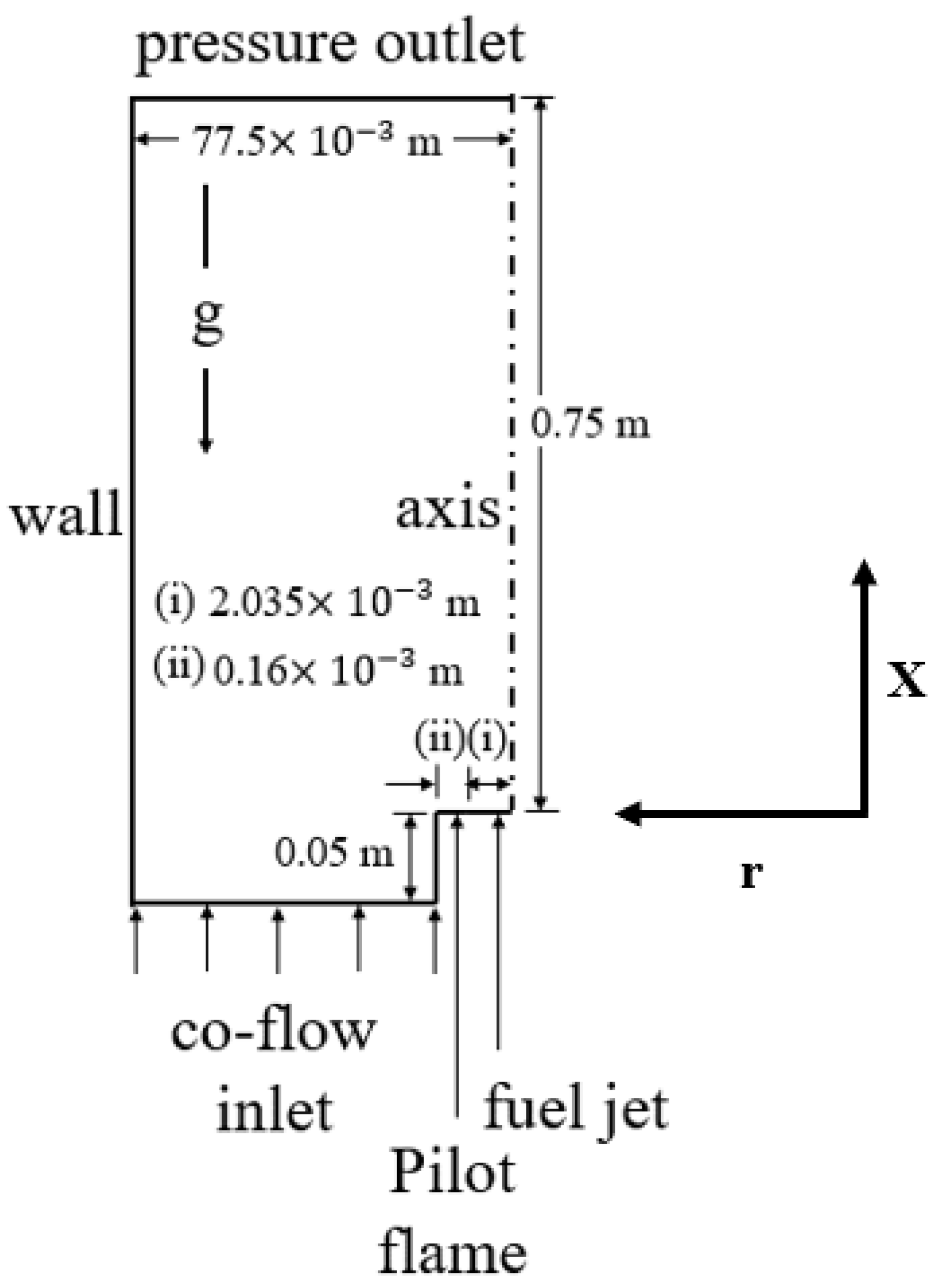
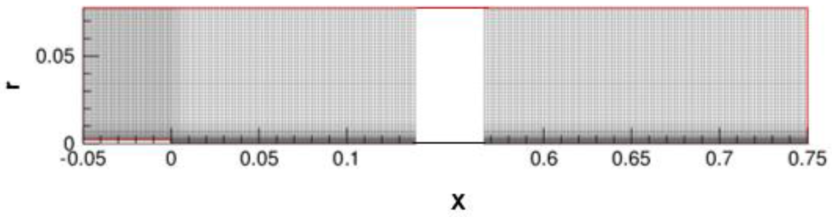
2.1. Physical Description of the Geometry and Grid Details

The details of the computational domain are shown in Figure 1. The geometrical configuration of the computational domain was adopted from the experimental test rig of Brookes and Moss [10]. Due to the symmetry of the geometry, we have considered a two-dimensional axisymmetric computational domain. Many researchers [18,19,20,21,34] have considered an axisymmetric computational domain for such type of geometry. It consists of a central fuel jet and a co-flow air jet. The diameter of the fuel jet at the inlet was kept as 4.07 × 10⁻³ m. Pure methane (CH4) was considered as fuel while air (21% O2 + 79% N2 on a volume basis) was used as an oxidizer. An annular co-flow pilot flame of width 0.16 × 10⁻³ m surrounding the fuel jet was considered for flame stabilization. The computational domain begins from the inlet of the fuel nozzle and extends up to 0.75 m in the axial direction and 77.5 × 10⁻³ m in the radial direction. Air was supplied at the co-flow inlet, which was placed at a location of 0.05 m upstream of the fuel nozzle. The air temperature was varied from 293 to 723 K to evaluate the effect of preheated air on soot formation and flame structure.
Structured quadrilateral elements of non-uniform size were considered to mesh the computation domain, as shown in Figure 2. To achieve this task, Ansys ICEM CFD 19.2 was used. A grid sensitivity test was performed to obtain the minimum number of cells necessary beyond which the results are independent of the mesh size. The grid convergence test was conducted by considering four different mesh sizes based on the axial variation of temperature at 1 and 3 atm. A final grid of 62,400 cells was chosen as the grid-independent solution, and further simulations were carried out with this grid.

2.2. CFD Modelling

The general form of the Favre-averaged governing equations for the variable ϕ in the Cartesian form of tensor notation is written as:
t ( ρ ¯ ϕ ˜ ) + x j ( ρ ¯ u j ˜ ϕ ˜ ) = x j ( Γ ϕ ϕ ˜ x j ) + S ϕ
where ρ ¯ is the mean density and ϕ ˜ is the Favre averaged scalar in the turbulent flow field. The Favre averaged velocity in jth coordinate is represented by u j ˜ . Γ ϕ and S ϕ in the equation represent the diffusion co-efficient and source term of the scalar ϕ ˜ , respectively. The corresponding value of the scalar ϕ ˜ , the diffusion coefficient Γ ϕ , and the source term S ϕ in the governing equations are listed in Table 1.
The Favre averaged governing equations (refer to Equation (1) and Table 1) were solved in the computational domain. A steady pressure-based solver was used to model the fluid flow by CFD simulation. Standard κ ε model was considered for turbulence modeling where two separate equations of turbulent kinetic energy and its dissipation rate were solved (refer to Table 1). The empirical constant C ε 1 in the transport equation of turbulent dissipation rate was changed from its default value of 1.44 to 1.6 following the work of [34,35,36]. The near-wall physics was captured using scalable wall function. Incompressible ideal gas law was used to calculate the densities. The gravity term was taken in the negative X-direction of the momentum equations.

2.2.1. Turbulence-Chemistry Interaction

The chemical reaction kinetics and its interaction with turbulence were modeled using a steady laminar flamelet model. The steady laminar flamelet model assumes the turbulent flame as an ensemble of laminar, one-dimensional local structures. The model computes the Favre averaged transport equations of mean mixture fraction and its variance as listed in Table 1 [37,38]. Counter-flow configuration of laminar diffusion flame is used to represent the thin reactive-diffusive layer in the turbulent flow field. The laminar counter-flow diffusion flame equations can be transformed from physical space to mixture fraction space to represent the reactive-diffusive layer. The flamelet equation for the species mass fraction and temperature can be derived by application of a universal co-ordinate transformation and subsequent asymptomatic approximation (where the scalars Yi and T are expressed as mixture fraction f).
ρ Y i t = 1 2 ρ χ 2 Y i f 2 + S i
ρ T t = 1 2 ρ χ 2 T f 2 1 c p i h i S i + 1 2 C p ρ χ [ C p f + i c p , i Y i f ] T f
The species mass fractions are mapped from mixture fraction space to physical space with the help of the mixture fraction and scalar dissipation rate. GRI Mech 3.0 [39] was used to represent the chemistry and to calculate the species source term. The scalar dissipation rate quantifies the deviation of equilibrium and is defined as
χ = 2 D | f x j | 2
The scalar dissipation rate varies along the flamelet. The flamelet strain rate ( a s ) can be related to the scalar dissipation rate (χ) at the position where f is stoichiometric [40] and is given by
χ s t = a s e x p ( 2 [ e r f c 1 ( 2 f s t ) 2 ] ) π
The ensemble of diffusion flamelets is used to represent the flame brush. The Favre averaged species mass fraction and temperature for a turbulent flame can be determined as
ϕ ˜ = ϕ   ( f , χ s t ) p ( f , χ s t ) d f d χ z t
The temperature and mean density have an extra dimension of mean enthalpy H ˜ to consider the non-adiabatic extension of steady diffusion flamelets. The species mass fraction is assumed to have a negligible effect by the heat loss or gain by the system. A presumed β-PDF distribution was used to define the probability of mixture fraction. The PDF for χ is the delta function assuming that fluctuations are neglected. The mean scalar dissipation rate Χ ˜ was modeled as
Χ ˜ = c Χ ε ˜ κ ˜ f ˜ 2
here, c Χ is a constant having a value of 2.0 [41]. Computational expensive calculations were pre-processed and stored in look-up tables. The advantage of this model is the calculation of a reactive flow field with a detailed kinetic mechanism by solving only two additional transport equations for the mean mixture fraction and mixture fraction variance. The flamelet controls and parameters used in Ansys Fluent 19.2 for the calculations are listed in Table 2 and Table 3. Similarly, the parameters used in the generation of PDF are given in Table 4.

2.2.2. Radiation Modeling

The discrete ordinate radiation model (DO model) [42] was used to evaluate the heat transfer due to radiation. In the discrete ordinate method, a discrete representation of the directional variation of the radiation intensity is used. The radiative transfer equation was evaluated for a set of n-discrete directions ( s ^ k , k = 1, 2, 3……n) than spans over the entire range of solid angle 4 π . The scattering effect was neglected since the particles in the flame are extremely fine and well dispersed. The reduced form of the radiative heat transfer equation is given as:
s ^ k . I k = a ( I b I k )
here I k is the radiation intensity in the kth direction, I b is the blackbody radiation intensity, and a is the absorption coefficient.
The bulk gas is considered as the participating media, since the product gases, especially CO2 and H2O, have higher emissivity. Moreover, soot has very high emissivity as it is considered as a black body. Weighted sum grey gas model with suitable weighing factor [43] was implemented to calculate absorption co-efficient of bulk gases as
a g a s = l n [ 1 i = 0 I a ε , i ( T ) ( 1 e k i P S ) ] S
where, a ε , i represent the emissivity-weighting factor for the ith grey gas as based upon gas temperature, T. k i denotes the absorption coefficient of the i-th grey gas. P is the sum of partial pressures of all-absorbing gas, and S is the path length.
The emissivity weighting factor,   a ε , i is a polynomial function of temperature and represented as
a ε , i = j = 1 J b ε , i , j T j 1
here, b ε , i , j is the emissivity gas temperature co-efficient. The value of co-efficient b ε , i , j , and k i were considered from the work of Smith et al. [43].
The fraction of the absorption coefficient contributed by soot is a linear function of temperature and evaluated as [44]:
a s o o t = 1232.4 ρ s o o t [ 1 + 4.8 × 10 4 ( T 2000 ) ]
hence, the effective absorption coefficient is
a = a g a s + a s o o t

2.2.3. Soot Modelling

In the present work, Moss–Brookes model [12] was used to calculate the rate of soot formation in a turbulent flame. In this model, two transport equations for the soot number density (N) and the soot mass concentration (M) were solved. The source term for number density (N) was evaluated by taking into account of nucleation and coagulation of soot particles and is given as:
d N d t = C α N A ( X p r e c P R T ) e x p ( T α T ) N u c l e a t i o n C β ( 24 R T ρ s o o t N A ) d p s o o t 1 / 2 N 2 C o a g u a l t i o n
Similarly, the source term for mass concentration (M) was calculated by considering nucleation, surface growth, and soot oxidation and is given as:
d M d t = C α M P ( X p r e c P R T ) e x p ( T α T ) N u c l e a t i o n + C γ ( X s g s P R T ) e x p ( T γ T ) [ ( π N ) 1 / 3 ( 6 M ρ s o o t ) 2 / 3 ] n S u r f a c e   g r o w t h [ C o x i d C ω , 1 η c o l l ( X O H P R T ) T ( π N ) 1 / 3 ( 6 M ρ s o o t ) 2 / 3 + C o x i d C ω , 2 ( X O 2 P R T ) e x p { T ω 2 T } T ( π N ) 1 / 3 ( 6 M ρ s o o t ) 2 / 3 ] O x i d a t i o n
Acetylene (C2H2) was considered a soot precursor for both nucleation and surface growth in the above equations. The oxidation model proposed by Lee et al. [45] was used in which, along with OH, the effect of O2 was considered to calculate the oxidation rate. The concentration of OH was determined using a partial equilibrium approach, while the concentration of O-radicals was calculated by considering the equilibrium approach. The turbulence-chemistry interaction on soot formation was calculated using a probability distribution function in mixture fraction. In this approach, the PDF look-up table provides the instantaneous values for species concentration and temperature which are a function of mixture fraction. For each cell, the soot production rate and enthalpy at each instant are computed. The mean mixture fraction and variance for each cell are used to compute the PDF table for the mixture fraction. The instantaneous soot rates are convoluted with the mixture fraction PDF to yield the mean rates in a turbulent flow. Soot-radiation interaction was enabled in the soot model so that the soot equations are solved together with the combustion solution to obtain correct radiation coupling [44].
In Equations (13) and (14), the model constants C α , C β and C γ are 54 s 1 , 1.0 and 11,700 kg·m·kmol−1·s−1, respectively. NA ( = 6.022045 × 10 26   Kmol 1 ) is the Avogadro number, and X p r e c is the mole fraction of soot precursor (C2H2 for methane flames). T α is the activation temperature for the nucleation reaction with a value of 21,000; as given by Lindstedt [46], ρ s o o t (=1800 kg/m3) is the mass density of soot, dp is the mean diameter of the soot particles. The activation temperature for surface growth rate ( T γ ) was considered with a value of 12,100 K by Leung et al. [47]. The soot oxidation model constants C ω , 1 and C ω , 2 are 105.81 kg·m · kmol 1 · K 1 / 2 s 1 , 8903.51 kg·m · kmol 1 · K 1 / 2 s 1 , respectively, along with a T ω , 2 value of 19,778 K. The collision efficiency ( η c o l l ) of 0.04 was considered following the earlier investigation [12,13]. The oxidation scaling parameter was assumed with a value of 0.015.

2.3. Boundary Condition

The formulation of the problem was completed by imposing appropriate boundary conditions in the computational domain. The wall of the combustor was set adiabatic. At the inlet fuel and co-flow air, mass flow inlet boundary conditions were imposed. The combustor centerline was given axis boundary condition. The inlet of the pilot flame was treated as an adiabatic wall. Previous investigations by [16,48] excluded pilot flame from their computation. The operating conditions used in the experimental investigation by Brookes and Moss [10] were considered in the present work while the air temperature was varied from 293 to 723 K. The detailed operating conditions used in the present work are listed in Table 5.

2.4. Solution Methodology

The Favre averaged governing equations (refer Equation (1) and Table 1) along with prescribed boundary conditions were solved using finite volume-based multigrid solver Ansys Fluent 19.2 [39]. The convective terms in the governing equations are discretized using a second-order upwind scheme. A central difference scheme was used to discretize the diffusive part of the governing equations. Pressure and velocity were coupled using the Semi-Implicit Method for Pressure-Linked Equations (SIMPLE algorithm) [49]. The solution was considered to have reached convergence when all of the following conditions were satisfied.
(i)
The scaled residuals of all the equations, except the energy equation, were less than 10−6. For the energy equation, a stricter convergence criterion of 10−8 was maintained.
(ii)
The temperature variation at the exit of the combustor was less than 1 K.

2.5. Combustion Parameters

Fuel jet Reynolds number:
Re f = ρ f u f d f μ f
Co-flow jet Reynolds number:
Re c = ρ c u c d c μ c
where, the symbols ρ , u, d, and μ represent the density, average velocity, diameter, and viscosity at the inlet. Subscript f and c denote for the corresponding fuel and co-flow air jet.
Initial Fourier number: it is used to set the first timestep for the solution of the flamelet Equations (2) and (3).
Soot number density (N): It is the number of soot particles per unit volume.
Soot volume fraction
( f v ) : f v = N × π 6 d p 3
In Equation (17), dp is the mean diameter of soot particles.

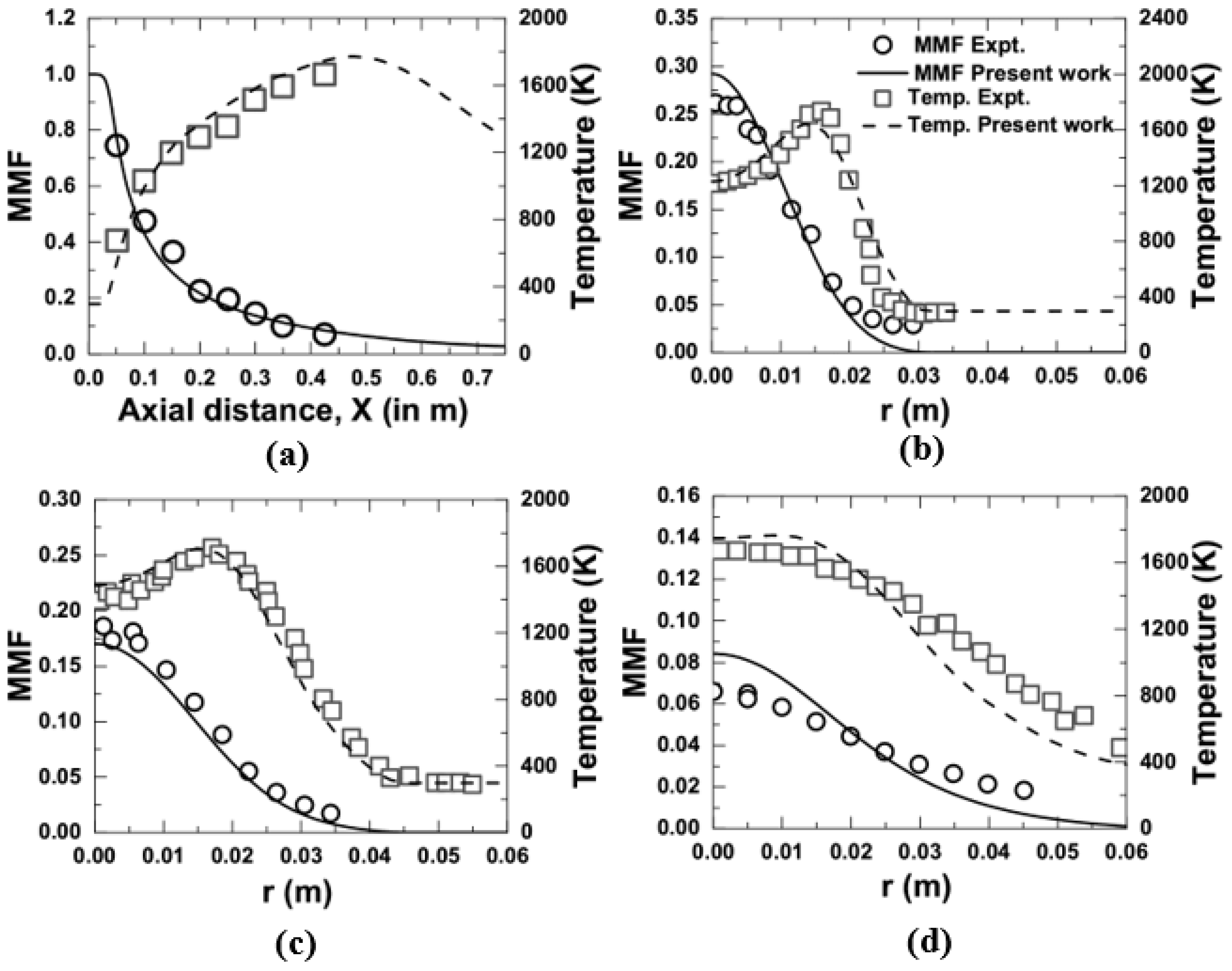
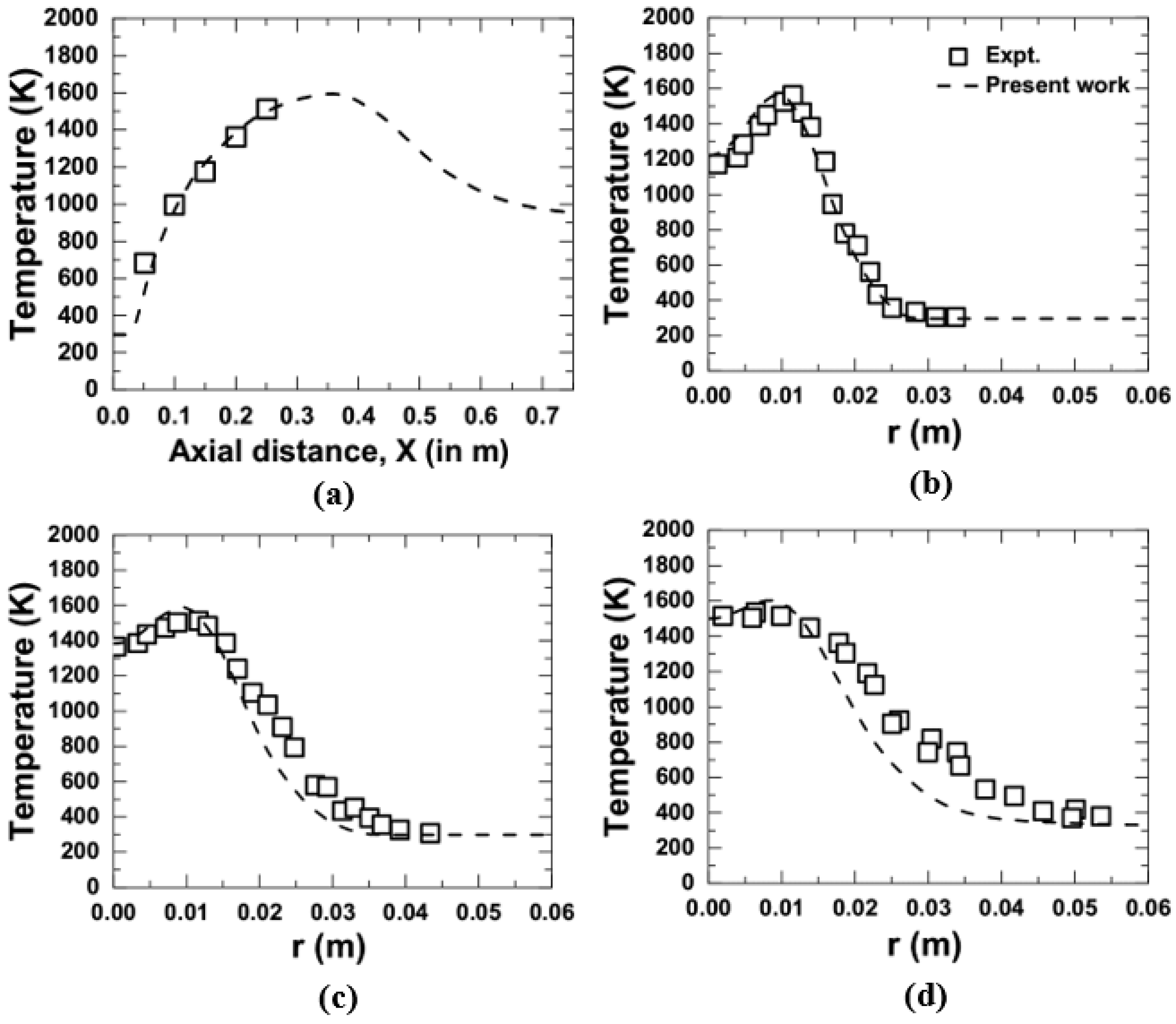
2.6. Validation Work

It is necessary to establish the accuracy and reliability of any computational method before any significant conclusion can be obtained from its results. The reliability of the solution was verified by ensuring the ability of the numerical formulation and solution method to accurately capture the complex physics involved in the problem. In the present work, the results obtained from the CFD simulation were compared with the measurement by Brookes and Moss [10]. The validation work was performed in two steps; (i) comparison of axial and radial variation of temperature and mean mixture fraction at 1 and 3 atm, and (ii) soot model validation by comparing the axial and radial variation of soot volume fractions at atmospheric and an elevated pressure of 3 atm.
(i)
Comparison of Mean Mixture Fraction and Temperature
The predicted CFD data of mean mixture fraction and temperature in the present computation were compared with the measurement [10] and are shown in Figure 3 and Figure 4. Figure 3a represents the axial variation, while Figure 3b–d shows the radial variation at an axial location of 0.15, 0.35, and 0.425 m, respectively, at 1 atm. It was noticed that the present computational approach was successfully able to capture the measured trend of temperature and mean mixture fraction along the centerline, as well as radially, with excellent agreement while operating at 1 atm. In the same way, at an elevated pressure of 3 atm, a comparison is presented in Figure 4a–d for the variation of temperature along the centerline and the radial direction for an axial location of 0.15, 0.2, and 0.25 m, respectively. The measurement for the variation of mean mixture fraction at 3 atm is not available in the literature of Brookes and Moss [10]. Hence, only the temperature variation was considered for comparison purposes. It was observed that the data obtained by the present computation for the temperature variation at 3 atm give a good prediction over the measurement.
(ii)
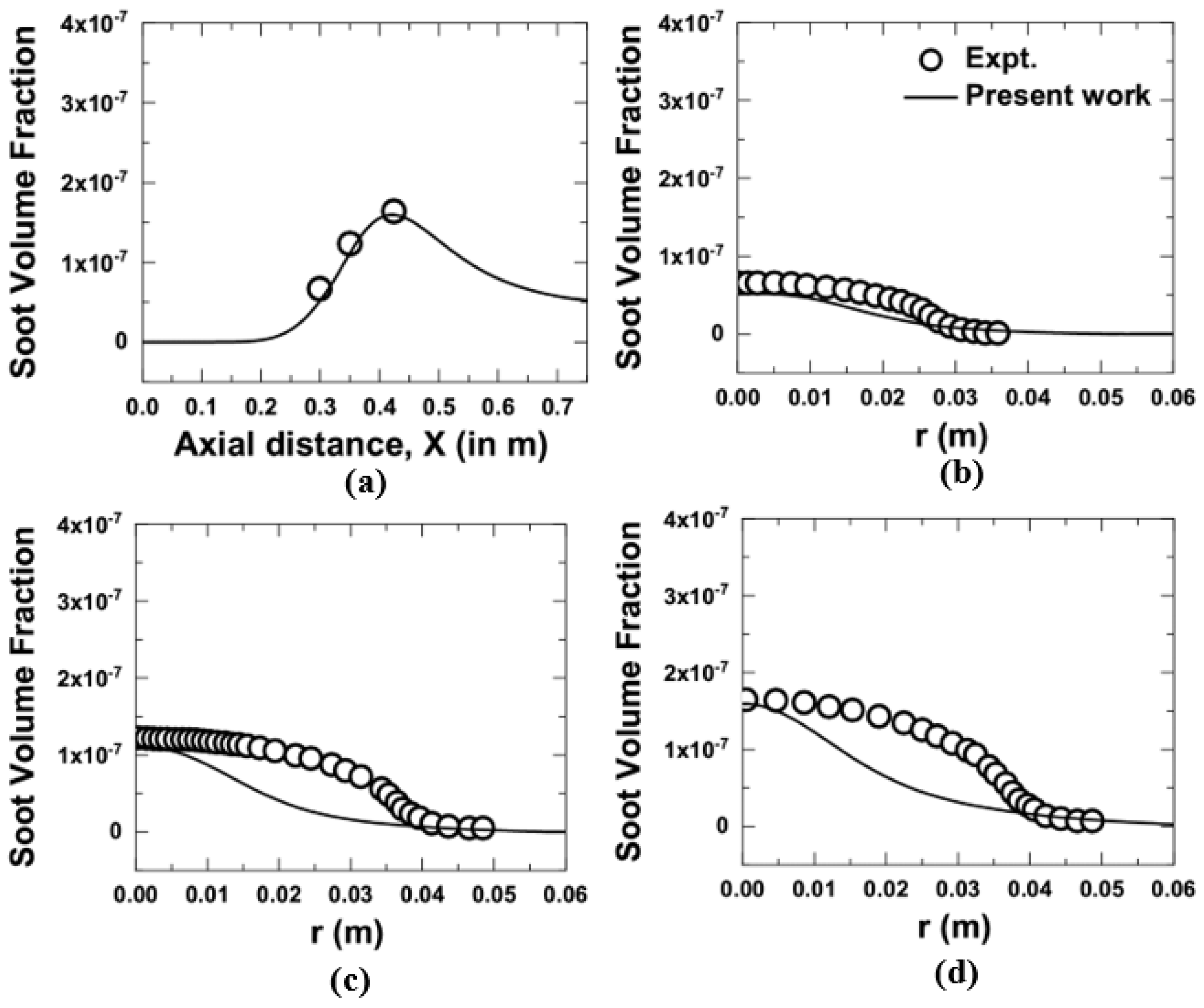
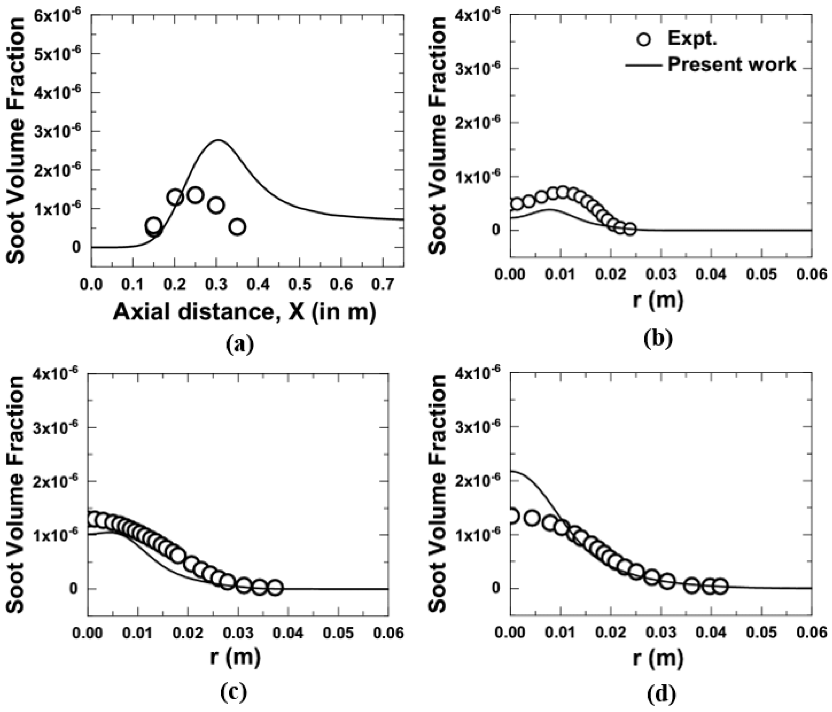
Comparison of Soot Volume Fraction at 1 and 3 atm
Figure 5 and Figure 6 shows the comparison for the variation of soot volume fraction obtained from the computation with the measurements [10] at 1 and 3 atm. The soot model by Brookes and Moss [12] was considered for the evaluation. It is to mention here that the model constants used in the soot model were not changed during the entire computation. The centerline variation of soot volume fraction for both the measurement and the computation at 1 atm is shown in Figure 5a, which showed excellent agreement. Figure 5b–d shows the radial variation of soot volume fractions for 1 atm at an axial location of 0.15, 0.35, and 0.425 m, respectively. It was observed that the numerical evaluations were able to capture the peak value reasonably well while slightly under prediction was noticed along the radial direction at a higher axial location of 0.35 and 0.425 m.
At an elevated pressure of 3 atm, the CFD predictions along the centerline for soot volume fractions gave good agreement up to 0.22 m and slightly over-predicted beyond 0.22 m, as shown in Figure 6a. The peak soot volume fraction obtained from CFD calculation was over-predicted by a factor of 2 (refer Figure 6a). The maximum soot volume fractions by the present numerical work were seen at an axial location of 0.31 m, i.e., 0.06 m further downstream from the measurement. Similarly, the radial variation of soot volume fractions at an axial location of 0.15, 0.2, and 0.25 m, respectively, for 3 atm is shown in Figure 6b–d. The computed soot volume fraction showed good agreement with the experimental data, while some major differences were noticed between the computations and measurements in terms of the peak value of the soot volume fraction. The peak soot volume fraction by calculation was under-predicted by a factor 2 and 1.2, respectively, as shown in Figure 6b,c. The calculated value of peak soot volume fraction in Figure 6b was located approximately at 0.0025 m upstream of the measured peak value. From Figure 6d, it was observed that the calculated peak soot volume fractions over-predicted the experimental data by a factor of 1.7. The soot volume fraction at 3 atm by measurement is ten times higher than 1 atm, correctly captured by the present numerical work.
Soot is a complex phenomenon and an exact match of the experimental result by modeling is very difficult to achieve. The soot formation model involving detailed chemical reaction mechanisms and aerosol dynamics to capture the complex processes of fuel pyrolysis, particle inception, growth, and oxidation are often too computationally expensive to be included in CFD simulation. It necessitates a less complex soot model such as an empirical or soot semi-empirical soot model that can be implemented in CFD simulation and give a soot prediction with reasonable accuracy. In the present work, the acetylene-based semi-empirical model proposed by Brookes and Moss [12] was considered. Many researchers [18,19] have implemented this soot model in CFD to predict soot volume fraction and to match with measurements. They also have observed a similar trend of CFD prediction like our present results.
From the overall analysis, it was found that the present computation was able to capture the combustion and sooting characteristics reasonably well and implemented in all cases considered in the present work.

3. Results and Discussion

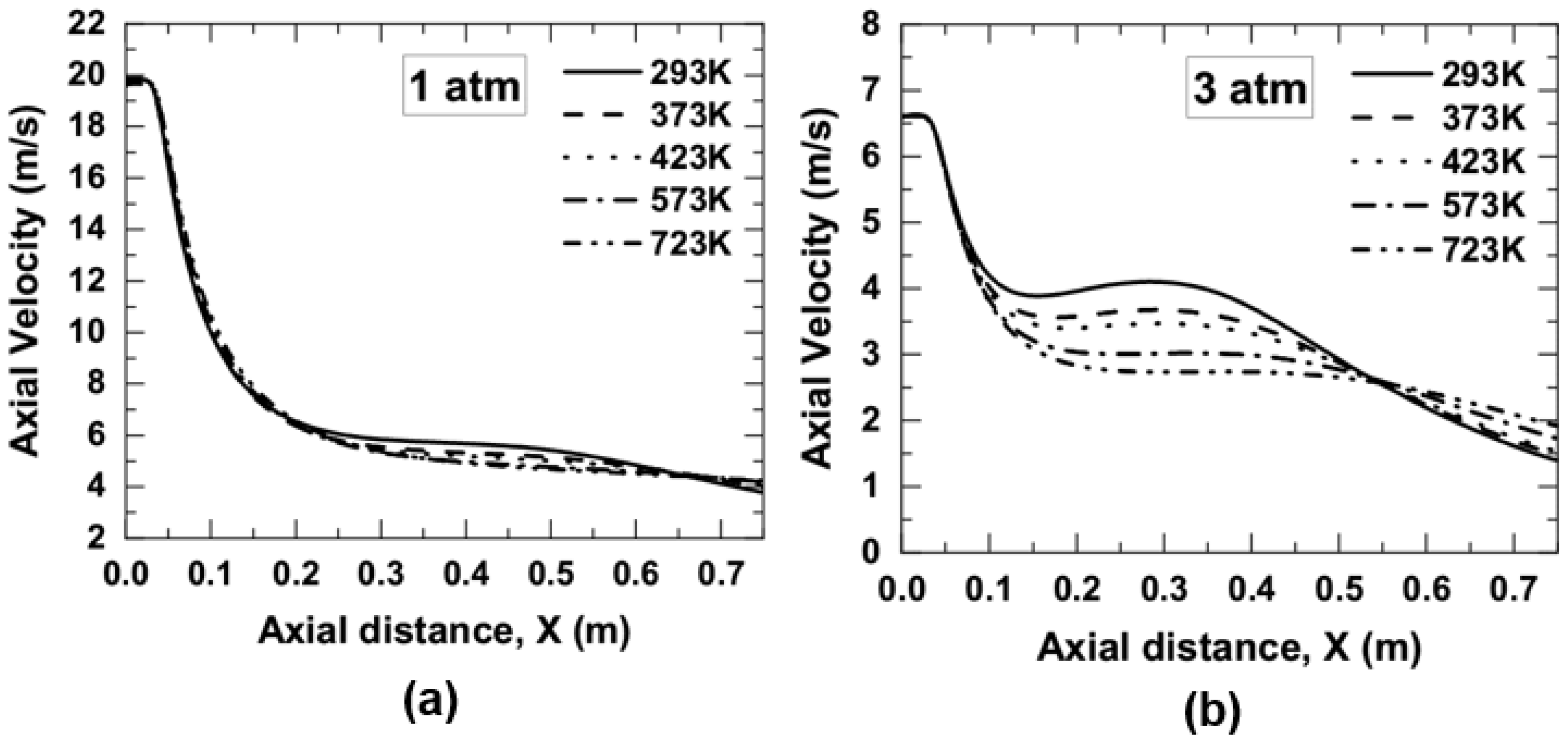
3.1. Axial Velocity and Residence Time

Effect of preheated oxidizer (air) temperature ranging from 293 to 723 K on the iso-line of axial velocity contour for two operating pressure of 1 and 3 atm are shown in Figure 7. An increase in oxidizer temperature increases the velocity at the co-flow inlet for a fixed mass flow rate of the oxidizer. The fuel jet velocity was held constant for a fixed pressure. The velocity was observed to vary only in the co-flow due to a change in the oxidizer temperature from 293 to 723 K. As the temperature of the oxidizer is increased, the buoyancy force is decreased (since density is decreased, ρ = P R T ). A decrease in buoyancy force may not pull the co-flow oxidizer stream effectively towards the centerline. Due to this, the axial velocity along the centerline is decreased. This was observed from Figure 7a, in which the iso-line of axial velocity (consider line corresponding to 5 m/s) was extended to a greater height at a low oxidizer temperature of 293 K, and with an increase in oxidizer temperature, the iso-line of axial velocity (say 5 m/s) was moved up to a shorter height. Similar observation can be obtained from an elevated pressure of 3 atm, as shown in Figure 7b. The iso-line of axial velocity (consider 3 m/s lines) was noticed to have extended to an increased height at 293 K than its counterparts at 723 K. Hence, the residence time of the mixture is increased with an increase in reactant temperature. Now, when it comes to comparing the cases between 1 and 3 atm pressure for a fixed reactant temperature, the iso-line of axial velocity (say 3 m/s) at atmospheric pressure was found at a greater height than 3 atm. This is due to the reduction of flow velocities with pressure since the mass flow rate of fuel and the oxidizer at the inlet are held fixed. Here, the velocities at the inlet of both the fuel and co-flow jet were decreased as the pressure was increased from 1 to 3 atm for a fixed air temperature. It shows a higher residence time at elevated pressure. Besides, the increased buoyancy force at elevated pressure (since density is increased) pulls the co-flow oxidizer stream towards the centerline and mixes with fuel, as observed from Figure 7b. It can be judged by isoline of axial velocity (say 1 m/s), which was observed to contract towards the centerline as the pressure was increased from 1 to 3 atm for a fixed reactant temperature.
The centerline variation of the axial velocity as a function of preheated air temperature for 1 and 3 atm pressure is shown in Figure 8. It was observed from Figure 8a,b that the axial velocity was greatly reduced in the range of axial position from 0.2 to 0.6 m for 1 atm and from 0.08 to 0.52 m for 3 atm. The buoyancy force at low temperatures is effectively higher than at high air temperature. Higher buoyancy force at low air temperature pulls the streamline from the co-flow air towards the burner centerline, mixes with the fuel, and increases the centerline flow velocity.

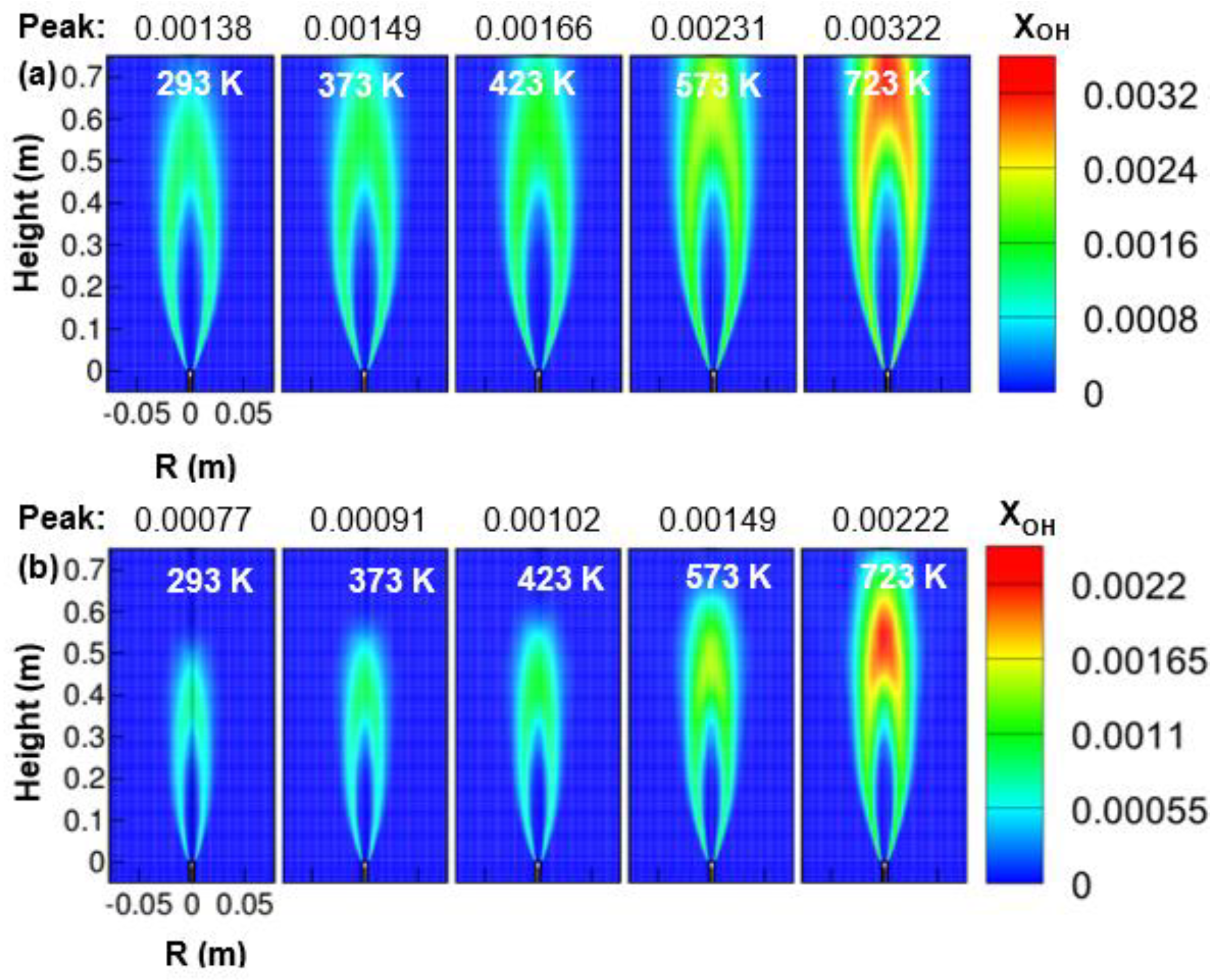
3.2. OH mole Fraction
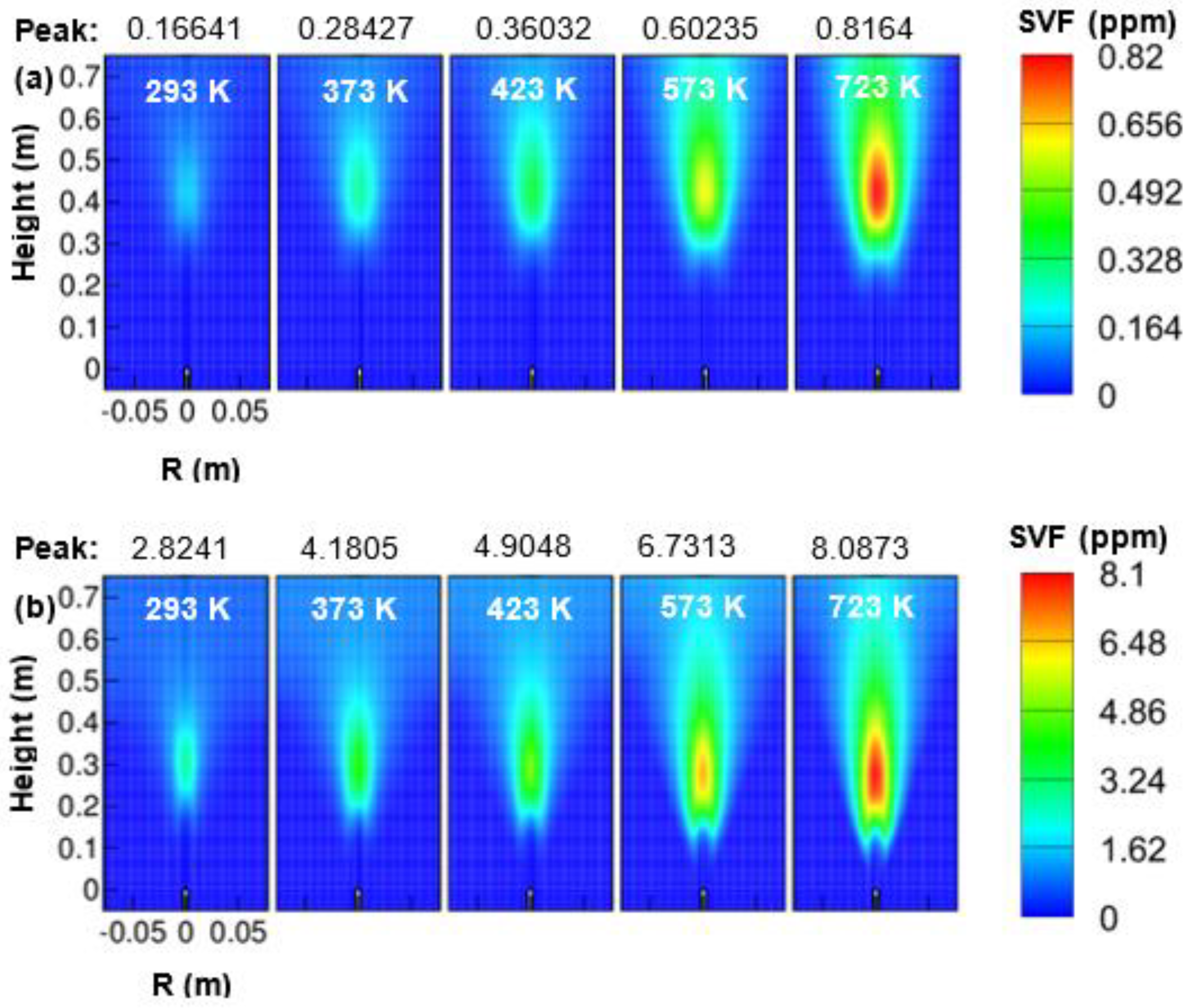
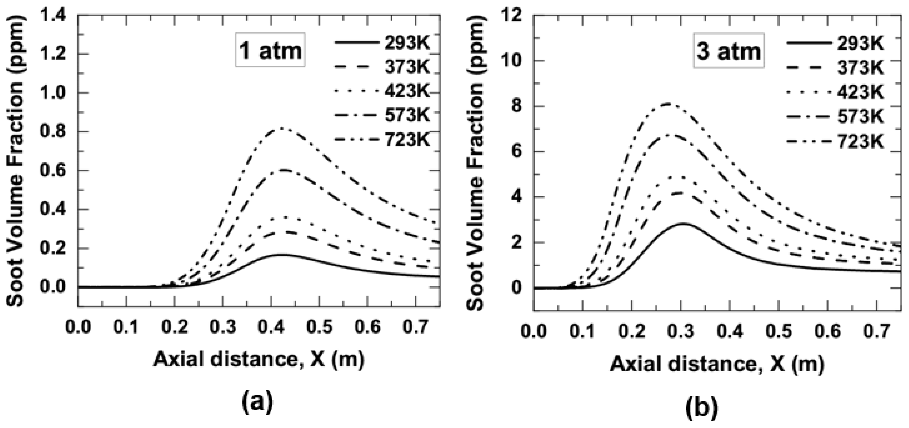
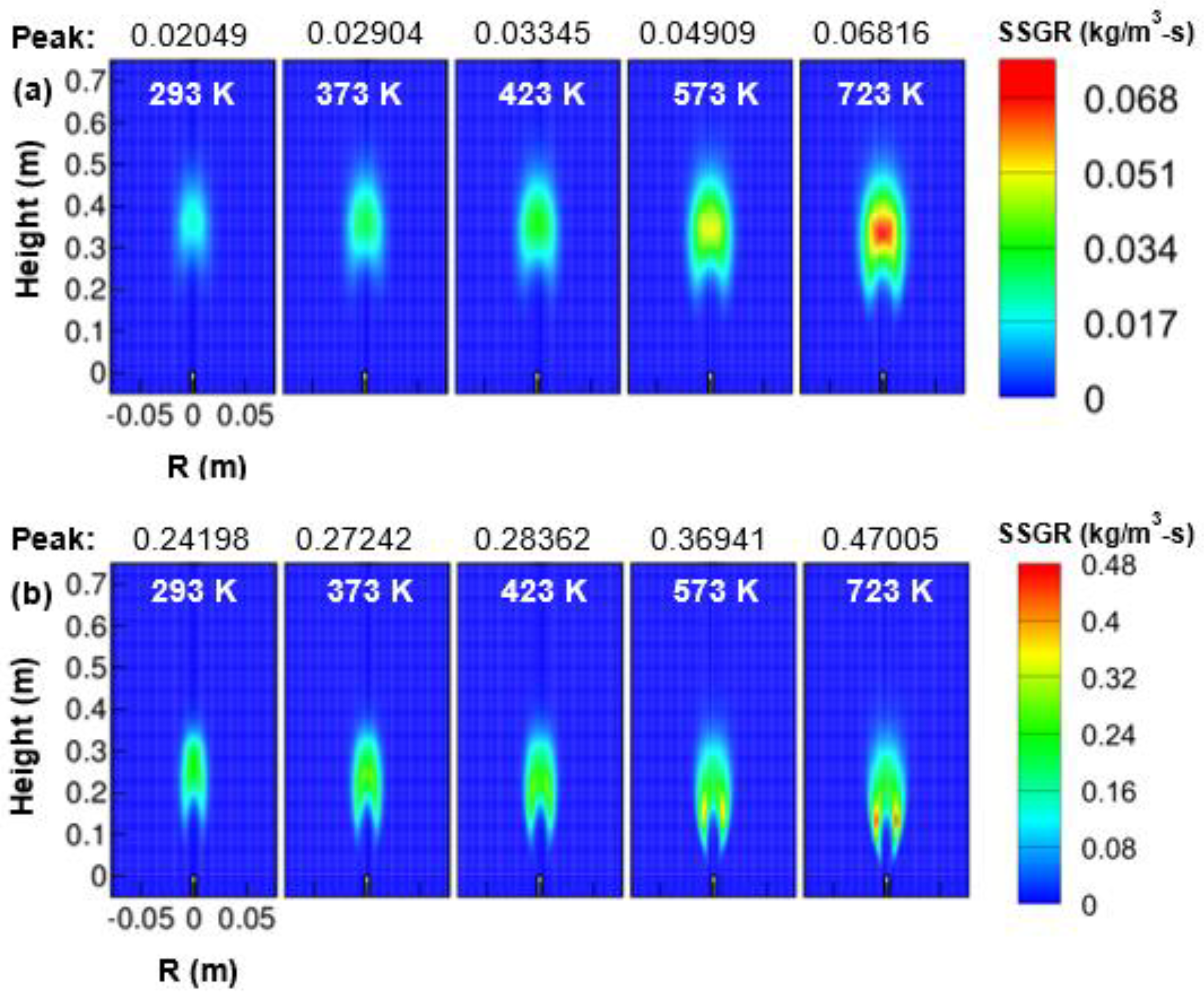
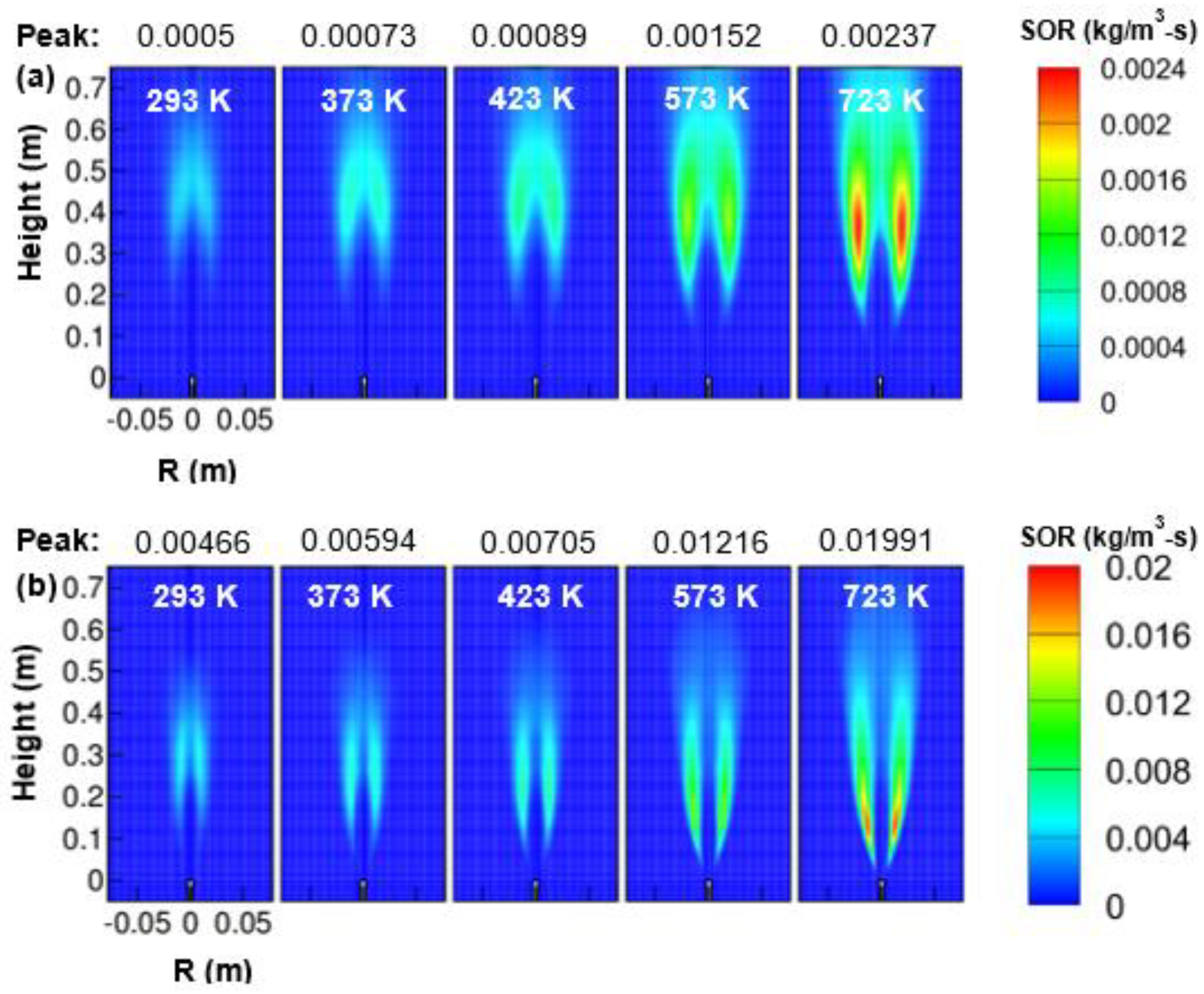
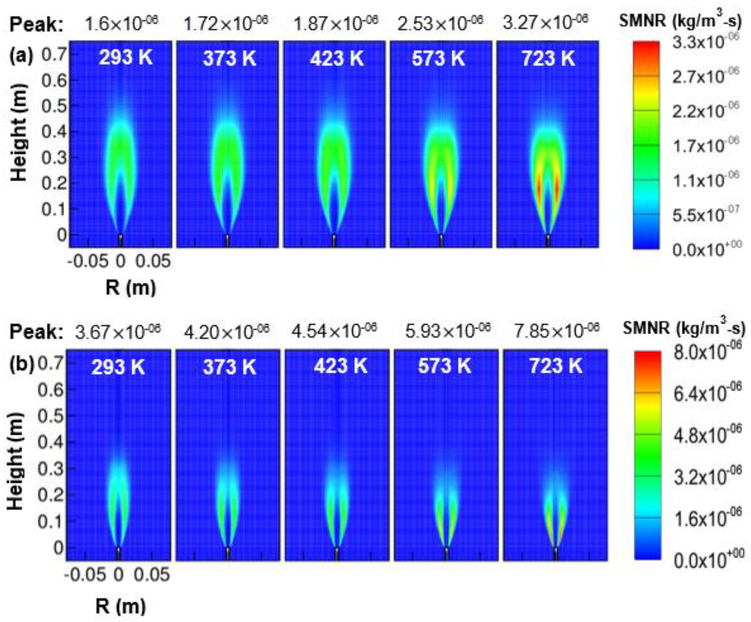
Figure 9a,b shows the contour plots of OH mole fractions obtained under the influence of preheated oxidizer temperature ranging from 293 to 723 K and for two operating pressure of 1 and 3 atm. The presence of OH species in the combustor determines the rate of reactions. It was seen that the OH mole fraction was increased when the oxidizer temperature was increased from 293 to 723 K. This shows an increase in reaction rate with the oxidizer temperature. Another observation from Figure 9 clearly shows the growth of the reaction zone with an increase in oxidizer temperature. The reaction zone got widened and elongated as the air temperature was increased from 293 to 723 K. Besides, the peak value of OH mole fraction moved downstream of the combustor as the temperature of the oxidizer increased. Further, the OH mole fraction at an elevated pressure of 3 atm showed a lower value than its corresponding counterparts at 1 atm while for a fixed reactant temperature. The reaction zone at 3 atm was also observed to be shorter and narrower than 1 atm. This may be because of the reduction of the flow velocity and the increased buoyancy force with pressure since the mass flow rate of the fuel and oxidizer at the inlet is kept fixed.

3.3. Soot

It can be observed from Figure 10 that the oxidizer temperature has a strong influence on the contour of the soot volume fraction at 1 and 3 atm. The peak soot volume fractions increased approximately linearly with air temperature both for 1 and 3 atm pressure. An increase in soot volume fraction with oxidizer temperature is mainly due to an increase in residence time. The increased residence time may have accumulated more fuel in the combustor. The soot volume fraction was seen broadened and elongated as the oxidizer temperature increased from 293 to 723 K. The buoyancy force becomes weak with increasing the oxidizer temperature. The buoyancy force usually forces the soot particle to get accumulated in a small space, i.e., around the centerline of the combustor. The entrainment of oxidizer to the flame is higher at 293 K, and it gets slowed down with an increase in oxidizer temperature. This might also be the reason behind an increase in soot volume fraction at high reactant temperature. The peak soot volume fraction was increased from 0.16 ppm at 293 K to 0.82 ppm at 723 K when the combustor was operated at 1 atm. At elevated pressure of 3 atm, the peak soot volume fraction showed a value that is 10 times higher than 1 atm while operating at fixed reactant temperature. A high value of soot volume fraction at elevated pressure is mainly due to an increase in residence time. As far as the effect of oxidizer temperature on peak soot volume fraction at 3 atm is concerned, the peak soot volume fraction was increased linearly from 2.82 ppm at 293 K to 8.08 ppm at 723 K.
Figure 11a,b demonstrated that a rise in air temperature leads to the early appearance of soot, and the soot was extended towards more combustor downstream. The peak soot volume fractions of 0.16 ppm were observed at 293 K which got increased to 0.81 ppm at 723 K when the combustor was operated at 1 atm. Similarly, the peak soot volume fractions were observed to increase from 2.82 ppm to 8.08 ppm as the air temperature was increased from 293 to 723 K, respectively. It indicated an increase in approximately 4.9 and 2.8 times in the axial peak value of soot volume fraction as air temperature increased from 293 to 723 K for both 1 and 3 atm, respectively. The results obtained from Figure 10 and Figure 11 also show that the peak value of soot volume fraction forms along the centerline of the combustor. There was no noticeable change in the location of peak soot-volume-fraction as the air temperature was increased from 293 to 723 K for 1 atm. The peak soot-volume-fraction was seen approximately at a position of 0.44 m for 1 atm. In the case of 3 atm, the peak value of soot volume fraction was seen to move slightly left, i.e., towards the combustor inlet with a rise in air temperature from 293 to 723 K. At 3 atm, the peak soot volume fraction was located approximately at 0.3 m at 293 K and 0.26 m at 723 K. As far as the effect of combustor pressure on the location of peak soot volume fraction is concerned, the location was seen to shift towards the combustor inlet with an increase in pressure from 1 and 3 atm for a fixed air temperature. For an instance, the peak soot volume fraction was observed to change its position from 0.44 m at 1 atm to 0.3 m at 3 atm for a fixed air temperature of 293 K.
The contour plots obtained for soot reaction rate by surface growth, oxidation, and mass nucleation are presented in Figure 12, Figure 13 and Figure 14. The soot mass additions take place more by surface growth rate than oxidation rate. Augmentation of the soot-surface growth rate was observed with a rise in air temperature. An expression for the soot surface growth can be observed from Equation (14). In addition, the soot surface growth rate got widened as the air temperature was increased from 293 to 723 K. It was observed from Figure 12 that the peak soot surface growth rate varied approximately as T a i r 1.31 for 1 atm pressure and linearly with air for 3 atm pressure. Another observation from Figure 5 clearly showed that the surface-growth-rate zone moved towards combustor upstream with an increase in air temperature. Next, the peak region of the surface growth rate was noticed in the central region for 1 atm and in the wings region at 3 atm (refer Figure 12a,b).
From Figure 13, it was observed that the soot-oxidation rate increased with an increase in oxidizer temperature for both 1 and 3 atm pressure. The peak soot oxidation rate was noticed to vary approximately as T a i r 1.72 for 1 atm pressure and as T a i r 1.63 for 3 atm pressure. The maximum value of the soot-oxidation rate was located at the wings region, not at the central region. The expressions for soot oxidation rate can be observed from Equation (14). As the air temperature was increased from 293 to 723 K, the peak soot oxidation rate was increased by approximately 4.74 and 4.27 times for the operating pressure of 1 and 3 atm, respectively. The reaction zone by soot oxidation rate at 723 K was also observed to be broader and longer than the corresponding zone at 293 K both for 1 and 3 atm. Further, the peak soot oxidation rate at elevated pressure was found more than at atmospheric pressure while for a fixed air temperature. The reaction zone obtained by soot-oxidation rate got narrowed as the combustor pressure was increased from 1 to 3 atm.
Figure 14a,b shows the soot-mass nucleation rate contour varying with air temperature from 293 to 723 K for two operating pressure of 1 and 3 atm. As the air temperature was increased from 293 to 723 K, the peak soot-mass nucleation rate was enhanced by approximately 2.05 and 2.15 times for the operating pressure of 1 and 3 atm, respectively. The peak region in the soot-mass nucleation rate was observed in the wing region for all cases of preheated air considered in the present work. The peak soot-mass nucleation rate was seen to vary with air temperature as T a i r 0.82 for 1 atm and T a i r 0.84 for 3 atm, respectively.

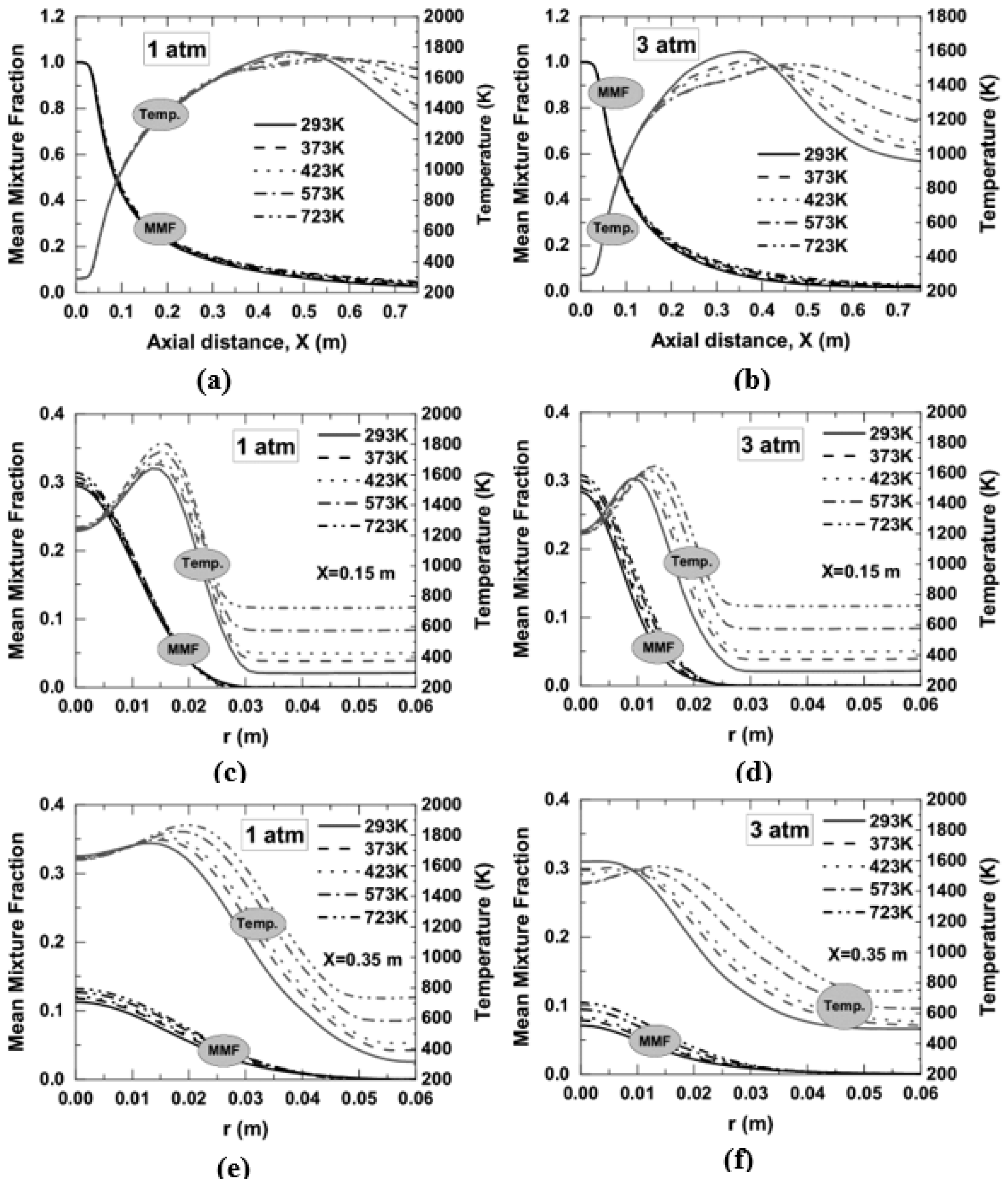
3.4. Temperature and Mean Mixture Fraction

Figure 15a,b shows the temperature contour obtained by varying the air temperature from 293 to 723 K and with the operating pressure of 1 and 3 atm. It was observed that an increase in oxidizer temperature increased the peak temperature of the combustor. A rise of maximum flame temperature of 101 K at 1 atm and 89 K at 3 atm were observed with an increase in air temperature from 293 to 723 K. It indicates a higher increment of peak temperature at 1 atm, and with an increase in pressure, the peak temperature increment gets lower. As the temperature of the air in the co-flow was increased, the flame was appeared to be broadened and elongated.
The axial variation of temperature along the centerline for two operating pressures of 1 and 3 atm is shown in Figure 16a,b. If attention is given to first Figure 16a, it was seen that with an increase in air temperature, the flame temperature was decreased in the range of axial distance approximately 0.34 to 0.55 m, and beyond 0.55 m, it shows an increasing trend. In the case of 3 atm, a reduction of flame temperature was observed in the range of approximately 0.15 to 0.45 m. Beyond 0.45 m, the flame temperature increases as the air temperature in the co-flow are increased from 293 to 723 K, as shown in Figure 16b. The region in which the flame temperature seems to be decreased, perhaps because of an increase in soot concentration in those regions (refer Figure 10). Usually, an increase in soot concentration helps in decreasing the flame temperature through radiation heat loss [8,10]. Similarly, the region with an increase in flame temperature is attributed to the increased reaction rate with air temperature (refer to Figure 9). The flame temperature was also observed to be higher in 1 atm than 3 atm. The reduced flame temperature at elevated pressure at 3 atm may be due to an increase in soot concentration ( 10 times higher than 1 atm) that leads to the radiative heat loss. The fuel consumption rate was decreased as the air temperature is increased; this can be observed from the profile of mean mixture fraction, as shown in Figure 16a–f. The decreased fuel consumption rate with an increase in temperature may be because of (i) a decrease in buoyancy force which has entrained less oxidizer stream towards the centerline to mix with the fuel, and (ii) an increase in residence time which has administered more fuel to the combustor. Similarly, the radial variation of temperature and mean mixture fraction at an axial location of 0.15 and 0.35 m and for 1 and 3 atm can be observed from Figure 16c–f. The flame peak temperature was not observed at the center, rather observed at a radial position of 0.015 m for 293 K, and as the air temperature was increased, the flame peak temperature was observed higher, and its position was shifted towards the right (refer Figure 16c). A similar thing concerning air temperature at 3 atm and an axial location of 0.15 m can be observed from Figure 16d. This shifting of flame peak position with air temperature indicates the widening of flame. As far as the effect of pressure on flame temperature is concerned, the flame peak position is shifted towards the centerline with an increase in pressure from 1 to 3 atm. This indicates the narrowing of flames with pressure for a fixed air temperature. Similarly, it was observed from the profile of the mean mixture fraction that the fuel consumption rate was decreased as the air temperature was increased since the fuel availability is increased with preheat temperature. By moving towards combustor downstream from 0.15 to 0.35 m, the fuel is consumed at a faster rate and spreading more radially outwards than the axial location of 0.15 m; the flame temperature is also radially more distributed at 0.35 m than 0.15 m (refer Figure 16e,f). The effect of pressure on the profile of the mean mixture fraction can be evaluated from Figure 16a–f. The mean mixture fraction was observed lower at 3 atm than at 1 atm for a fixed air temperature. This showed an increase in fuel consumption rate or the decreased availability of the fuel at elevated pressure for a fixed air temperature.

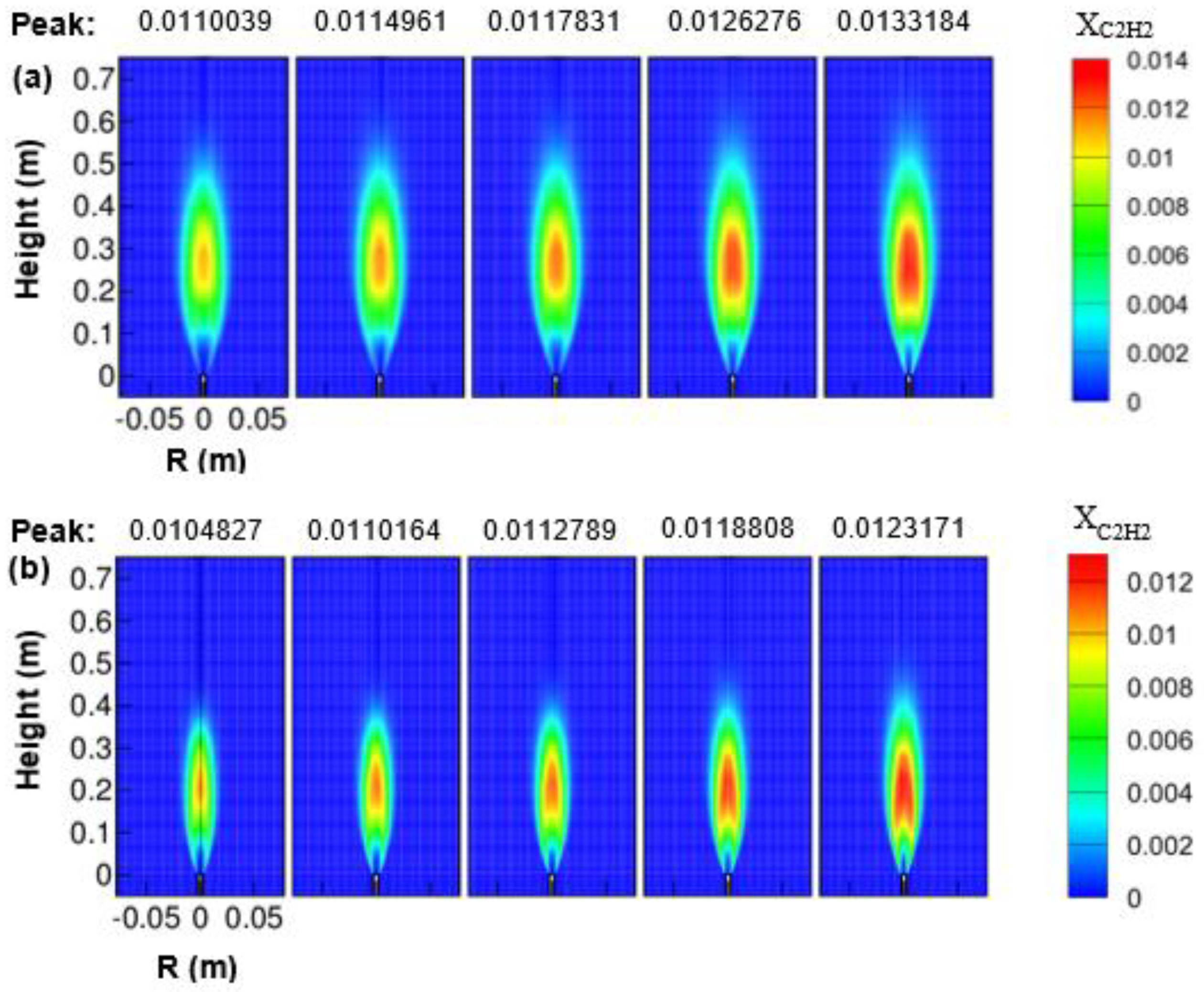
3.5. Acetylene Mole Fractions
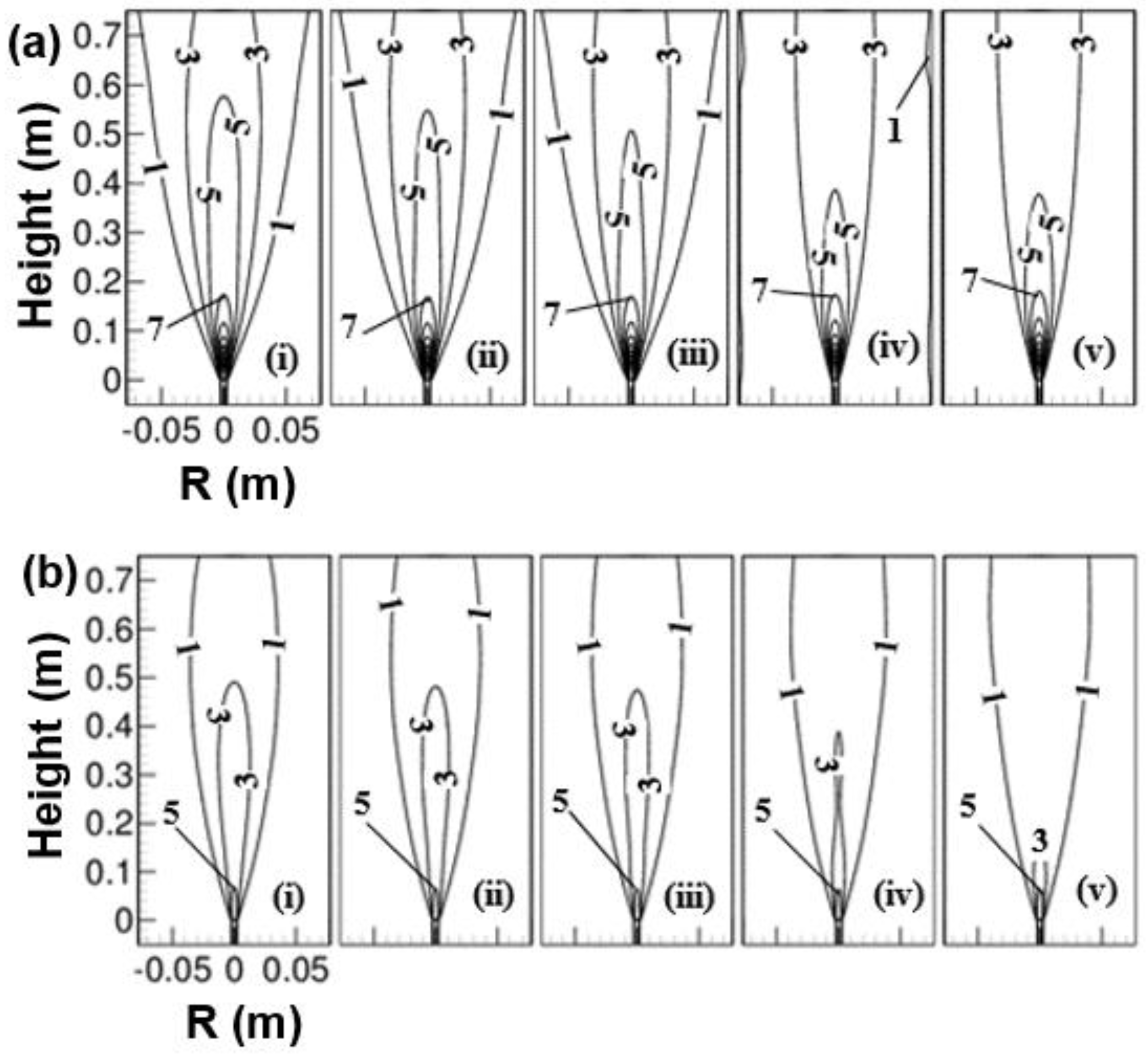
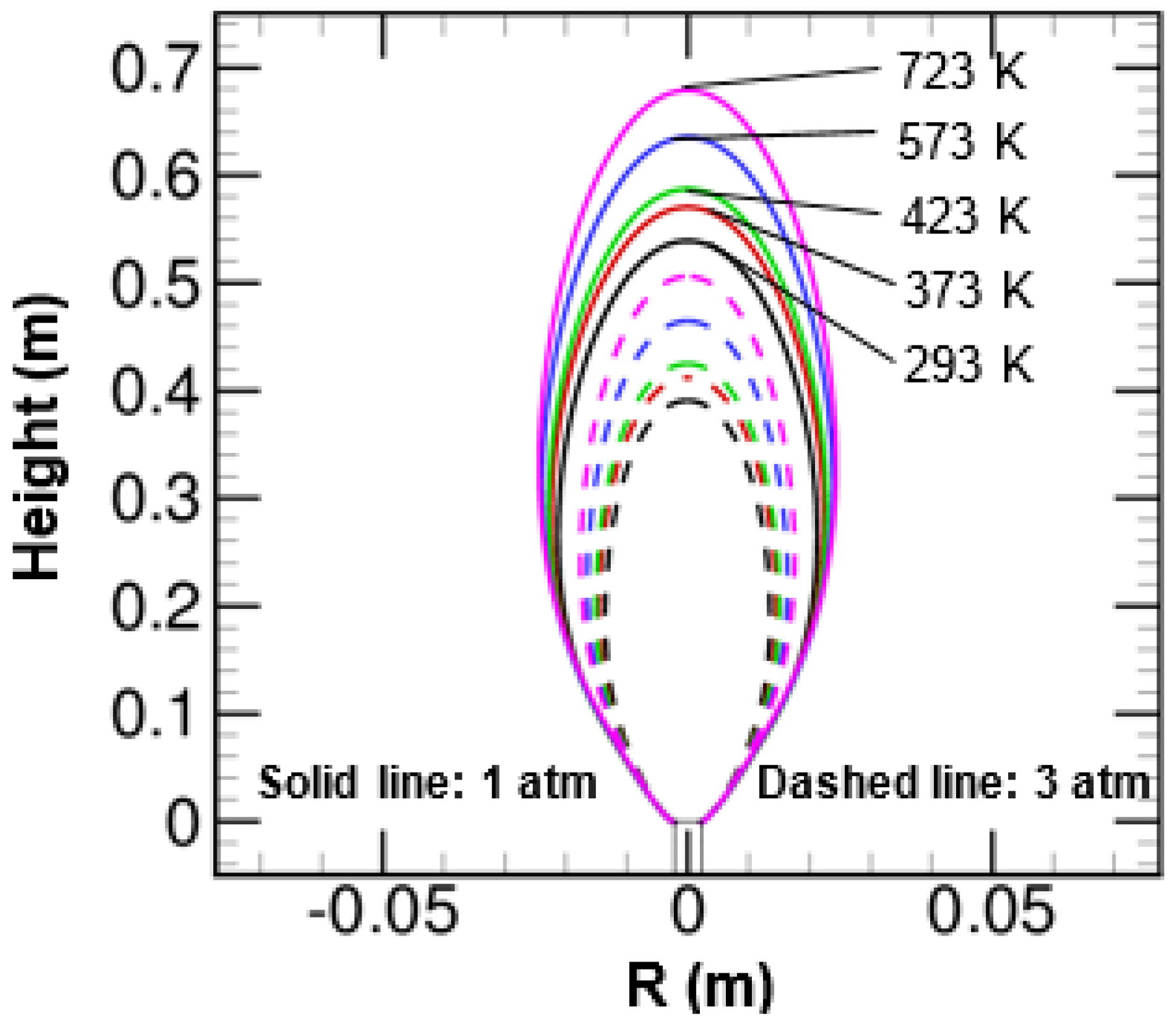
From Figure 17a,b, it was observed that the mole fraction of acetylene was increased as the air temperature was increased from 293 to 723 K both for 1 and 3 atm. This is expected since the fuel consumption rate is decreased, or the mean mixture fraction is increased with air preheat temperature. As the air temperature increases, the growth of the mole fraction of the acetylene reaction zone occurs that appears to be broadened and elongated. However, this is not the case when the effect of pressure is considered for a fixed reactant temperature. The acetylene mole fraction was seen to be decreased as the combustor pressure was increased from 1 to 3 atm. It may be due to the possibility of the decreased availability of the fuel in the combustor since the fuel is consumed at a faster rate at elevated pressure.

3.6. Flame Geometry

Figure 18 shows the effect of air temperature on flame geometry at two operating pressures of 1 and 3 atm. The flame geometry in Figure 18 is defined in terms of stoichiometric mixture fraction surface. The flames operating under atmospheric pressures are effectively wider and longer than the flames that operate at an elevated pressure of 3 atm. The narrowing and shortening nature of flames at 3 atm is mainly due to the increased buoyancy force as well as less value of velocity magnitude at this pressure than 1 atm. The active participation of buoyancy force usually helps in pulling the streamline or entraining the co-flow oxidizer stream towards the flame centerline. Apart from the pressure effect, the air temperature also has a substantial impact on the flame shape at two different pressure of 1 and 3 atm. The flame height was noticed to be increased with increasing air temperature for both 1 and 3 atm. The flame width also increased with air temperature. However, the increment was observed very marginally when compared with the flame height. The flame height was observed to vary with air temperature as T a i r 0.25 for 1 atm and as T a i r 0.32 for 3 atm. Similarly, the flame width was noticed to scale with air temperature as T a i r 0.2 for 1 atm and as T a i r 0.3 for 3 atm, respectively. The flame area was seen to vary with air temperature as T a i r 0.39 for 1 atm and T a i r 0.54 for 3 atm, respectively.

4. Conclusions

The effect of preheated oxidizer temperature on flame structure and sooting characteristics for turbulent methane/air diffusion flames at 1 and 3 atm were numerically investigated. The present investigation was conducted at 1 and 3 atm because the experimental data at these two pressures are available. The knowledge on the effect of preheated air temperature at atmospheric and at elevated pressures of 3 atm would also help the combustion researchers to carry out the MILD combustion investigation, since MILD combustion requires preheating of the reactants, and its application at high pressure is a challenging task as it involves many constraints like shorter ignition delay time. The oxidizer (air) temperature was varied from 293 to 723 K. The Favre averaged governing equations were discretized using the finite volume method and solved using Ansys Fluent 19.2. Standard k-ε turbulence model with modified empirical constant Cε1 = 1.6 was used to model the turbulence quantities. A steady diffusion laminar flamelet model coupled with the PDF method was used for combustion modeling. Detailed chemical mechanism GRI-Mech 3.0 was used for chemistry representation and to generate the flamelet. The acetylene-based semi-empirical soot model developed by Brookes and Moss was considered to calculate the rate of soot formation. The outcomes of the present computation are listed as follows:
(a)
The residence time of the fuel in the combustor gets decreased as the air temperature increases from 293 to 723 K and increases with pressure elevation. This occurs due to the influence of buoyancy force, which is a function of air temperature and combustor pressure. The buoyancy force is decreased with an increase in air temperature; however, it increased with a rise of combustor pressure.
(b)
The peak soot volume fraction is increased linearly with air temperature for both 1 and 3 atm while approximately 10 times higher at 3 atm than 1 atm. The reaction zone obtained by soot volume fraction also gets broadened and elongated with an increase in air temperature. The reaction rate by soot surface-growth, oxidation and nucleation rate is increased with both air temperature and combustor pressure.
(c)
The OH mole fraction, signifying reaction rate, increases with air temperature and decreases with pressure elevation. The flame height as well as the flame width increases as the air temperature increases from 293 to 723 K, while decreases at a higher pressure of 3 atm.
(d)
The fuel consumption rate decreases with an increase in air temperature for both 1 and 3 atm. However, it increases with pressure elevation while at fixed air temperature. This happens due to the change in residence time, influenced by air temperature and pressure.
Future work will focus on investigating the combustion and sooting characteristics at an extended pressure up to 10 atm as well as gaseous fuel other than methane.

Author Contributions

Conceptualization, S.G. and V.M.R.; methodology, S.G. and V.M.R.; software, S.M. and S.G.; validation, S.M. and S.G.; formal analysis, S.G. and V.M.R.; investigation, S.G., S.M., and V.M.R.; resources, V.M.R. and S.K.D.; data curation, S.M.; writing—original draft preparation, S.G.; writing—review and editing, V.M.R. and B.J.L.; visualization, B.J.L.; supervision, V.M.R. and S.K.D.; project administration, S.K.D. and B.J.L.; funding acquisition, B.J.L. and V.M.R. All authors have read and agreed to the published version of the manuscript.

Funding

This research received no external funding.

Institutional Review Board Statement

Not applicable.

Informed Consent Statement

Not applicable.

Data Availability Statement

Not applicable.

Acknowledgments

The authors would like to acknowledge the Indian Institute of Technology, India for providing computer and software facilities in the Computational Fluid Dynamics (CFD) laboratory at the Department of Mechanical Engineering. B.J.L. would like to acknowledge the support by the Korea Institute of Energy Technology Evaluation and Planning (KETEP) and the Ministry of Trade, Industry and Energy (MOTIE) of the Republic of Korea (Grant No. 20181110100290).

Conflicts of Interest

The authors declare no conflict of interest.

References

  1. Mishra, D.P.; Kumar, P. Experimental investigation of laminar LPG-H2 jet diffusion flame with preheated reactants. Fuel 2008, 87, 3091–3095. [Google Scholar] [CrossRef]
  2. He, Y.; Qi, S.; Liu, S.; Xin, S.; Zhu, Y.; Wang, Z. Effects of the gas preheat temperature and nitrogen dilution on soot formation in co-flow methane, ethane, and propane diffusion flames. Energy Fuels 2021. [Google Scholar] [CrossRef]
  3. Lim, J.; Gore, J.; Viskanta, R. A study of the effects of air preheat on the structure of methane/air counterflow diffusion flames. Combust. Flame 2000, 121, 262–274. [Google Scholar] [CrossRef]
  4. Chu, C.; Naseri, A.; Mitra, T.; Dadsetan, M.; Sediako, A.; Thomson, M.J. The effect of elevated reactant temperatures on soot nanostructures in a coflow diffusion ethylene flame. Proc. Combust. Inst. 2020, 38, 2525–2532. [Google Scholar] [CrossRef]
  5. Qi, S.; Sun, Z.; Wang, Z.; Liu, Y.; He, Y.; Liu, S.; Wan, K.; Nathan, G.; Costa, M. Effects of gas preheat temperature on soot formation in co-flow methane and ethylene diffusion flames. Proc. Combust. Inst. 2020, 38, 1225–1232. [Google Scholar] [CrossRef]
  6. Joo, H.I.; Guider, Ö.L. Soot formation and temperature field structure in co-flow laminar methane-air diffusion flames at pressures from 10 to 60 atm. Proc. Combust. Inst. 2009, 32, 769–775. [Google Scholar] [CrossRef]
  7. Liu, F.; Thomson, K.A.; Guo, H.; Smallwood, G.J. Numerical and experimental study of an axisymmetric coflow laminar methane-air diffusion flame at pressures between 5 and 40 atmospheres. Combust. Flame 2006, 146, 456–471. [Google Scholar] [CrossRef]
  8. Cao, S.; Ma, B.; Giassi, D.; Bennett, B.A.V.; Long, M.B.; Smooke, M.D. Effects of pressure and fuel dilution on coflow laminar methane–air diffusion flames: A computational and experimental study. Combust. Theory Model. 2018, 22, 316–337. [Google Scholar] [CrossRef]
  9. Karataş, A.E.; Gülder, Ö.L. Soot formation in high pressure laminar diffusion flames. Prog. Energy Combust. Sci. 2012, 38, 818–845. [Google Scholar] [CrossRef]
  10. Brookes, S.J.; Moss, J.B. Measurements of soot production and thermal radiation from confined turbulent jet diffusion flames of methane. Combust. Flame 1999, 116, 49–61. [Google Scholar] [CrossRef]
  11. Nishida, O.; Mukohara, S. Characteristics of soot formation and decomposition in turbulent diffusion flames. Combust. Flame 1982, 47, 269–279. [Google Scholar] [CrossRef]
  12. Brookes, S.J.; Moss, J.B. Predictions of soot and thermal radiation properties in confined turbulent jet diffusion flames. Combust. Flame 1999, 116, 486–503. [Google Scholar] [CrossRef]
  13. Kronenburg, A.; Bilger, R.W.; Kent, J.H. Modeling soot formation in turbulent methane-air jet diffusion flames. Combust. Flame 2000, 121, 24–40. [Google Scholar] [CrossRef]
  14. Yao, W.; Zhang, J.; Nadjai, A.; Beji, T.; Delichatsios, M. Development and Validation of a Global Soot Model in Turbulent Jet Flames. Combust. Sci. Technol. 2012, 184, 717–733. [Google Scholar] [CrossRef]
  15. Fairweather, M.; Jones, W.P.; Ledin, H.S.; Lindstedt, R.P. Predictions of soot formation in turbulent, non-premixed propane flames. Symp. Combust. 1992, 24, 1067–1074. [Google Scholar] [CrossRef]
  16. Wen, Z.; Yun, S.; Thomson, M.J.; Lightstone, M.F. Modeling soot formation in turbulent kerosene/air jet diffusion flames. Combust. Flame 2003, 135, 323–340. [Google Scholar] [CrossRef]
  17. Mohapatra, S.; Garnayak, S.; Lee, B.J.; Elbaz, A.M.; Roberts, W.L.; Dash, S.K.; Reddy, V.M. Numerical and chemical kinetic analysis to evaluate the effect of steam dilution and pressure on combustion of n-dodecane in a swirling flow environment. Fuel 2021, 288, 119710. [Google Scholar] [CrossRef]
  18. Reddy, M.; De, A.; Yadav, R. Effect of precursors and radiation on soot formation in turbulent diffusion flame. Fuel 2015, 148, 58–72. [Google Scholar] [CrossRef]
  19. Woolley, R.M.; Fairweather, M. Conditional moment closure modelling of soot formation in turbulent, non-premixed methane and propane flames. Fuel 2009, 88, 393–407. [Google Scholar] [CrossRef] [Green Version]
  20. Yadav, R.; Kushari, A.; Eswaran, V.; Verma, A.K. A numerical investigation of the Eulerian PDF transport approach for modeling of turbulent non-premixed pilot stabilized flames. Combust. Flame 2013, 160, 618–634. [Google Scholar] [CrossRef]
  21. Nmira, F.; Liu, Y.; Consalvi, J.L.; Andre, F.; Liu, F. Pressure effects on radiative heat transfer in sooting turbulent diffusion flames. J. Quant. Spectrosc. Radiat. Transf. 2020, 245, 106906. [Google Scholar] [CrossRef]
  22. Lakkis, I.; Ghoniem, A.F. Axisymmetric vortex method for low-Mach number, diffusion-controlled combustion. J. Comput. Phys. 2003, 184, 435–475. [Google Scholar] [CrossRef]
  23. Ogami, Y.; Fukumoto, K. Simulation of combustion by vortex method. Comput. Fluids 2010, 39, 592–603. [Google Scholar] [CrossRef]
  24. Heidarinejad, G.; Shahriarian, S. Simulation of premixed combustion flow around circular cylinder using hybrid random vortex. Int. J. Eng. Trans. B Appl. 2011, 24, 269–277. [Google Scholar] [CrossRef]
  25. Schlegel, F.; Ghoniem, A.F. Simulation of a high Reynolds number reactive transverse jet and the formation of a triple flame. Combust. Flame 2014, 161, 971–986. [Google Scholar] [CrossRef]
  26. Bimbato, A.M.; Alcântara Pereira, L.A.; Hirata, M.H. Development of a new Lagrangian vortex method for evaluating effects of surfaces roughness. Eur. J. Mech. B Fluids 2019, 74, 291–301. [Google Scholar] [CrossRef]
  27. Cavaliere, A.; De Joannon, M. Mild Combustion. Prog. Energy Combust. Sci. 2004, 30, 329–366. [Google Scholar] [CrossRef]
  28. Wünning, J.A.; Wünning, J.G. Flameless oxidation to reduce thermal no-formation. Prog. Energy Combust. Sci. 1997, 23, 81–94. [Google Scholar] [CrossRef]
  29. Reddy, V.M.; Biswas, P.; Garg, P.; Kumar, S. Combustion characteristics of biodiesel fuel in high recirculation conditions. Fuel Process. Technol. 2014, 118, 310–317. [Google Scholar] [CrossRef]
  30. Garnayak, S.; Elbaz, A.M.; Kuti, O.; Dash, S.K.; Roberts, W.L.; Reddy, V.M. Auto-Ignition and Numerical Analysis on High-Pressure Combustion of Premixed Methane-Air mixtures in Highly Preheated and Diluted Auto-Ignition and Numerical Analysis on High- Pressure Combustion of Premixed Methane- Air mixtures in Highly Preheated and D. Combust. Sci. Technol. 2021, 1–23. [Google Scholar] [CrossRef]
  31. Fortunato, V.; Giraldo, A.; Rouabah, M.; Nacereddine, R.; Delanaye, M.; Parente, A. Experimental and numerical investigation of a MILD combustion chamber for micro gas turbine applications. Energies 2018, 11, 3363. [Google Scholar] [CrossRef] [Green Version]
  32. Reddy, V.M.; Katoch, A.; Roberts, W.L.; Kumar, S. Experimental and numerical analysis for high intensity swirl based ultra-low emission flameless combustor operating with liquid fuels. Proc. Combust. Inst. 2015, 35, 3581–3589. [Google Scholar] [CrossRef] [Green Version]
  33. Dally, B.B.; Karpetis, A.N.; Barlow, R.S. Structure of turbulent non-premixed jet flames in a diluted hot coflow. Proc. Combust. Inst. 2002, 29, 1147–1154. [Google Scholar] [CrossRef]
  34. Christo, F.C.; Dally, B.B. Modeling turbulent reacting jets issuing into a hot and diluted coflow. Combust. Flame 2005, 142, 117–129. [Google Scholar] [CrossRef]
  35. Mardani, A.; Karimi Motaalegh Mahalegi, H. Hydrogen enrichment of methane and syngas for MILD combustion. Int. J. Hydrogen Energy 2019, 44, 9423–9437. [Google Scholar] [CrossRef]
  36. Chen, Z.; Reddy, V.M.; Ruan, S.; Doan, N.A.K.; Roberts, W.L.; Swaminathan, N. Simulation of MILD combustion using Perfectly Stirred Reactor model. Proc. Combust. Inst. 2017, 36, 4279–4286, ISBN 3981593693. [Google Scholar] [CrossRef] [Green Version]
  37. Peters, N. Turbulent Combustion; Cambridge University Press: Cambridge, UK, 2004. [Google Scholar]
  38. Versteeg, H.K.; Malalasekera, W. An Introduction to Computational Fluid Dynamics: The Finite Volume Method, 2nd ed.; Pearson Education: Harlow, UK, 2007. [Google Scholar]
  39. Smith, G.P.; Golden, D.M.; Frenklach, M.; Moriarty, N.W.; Eiteneer, B.; Gold-Enberg, M.; Bowman, C.T.; Hanson, R.K.; Song, S.; Gardiner, W.C., Jr.; et al. GRI-Mech 3.0. 2020. Available online: http://www.me.berkeley.edu/gri_mech/ (accessed on 2 January 2021).
  40. Peters, N. Laminar diffusion flamelet models in non-premixed turbulent combustion. Prog. Energy Combust. Sci. 1984, 10, 319–339. [Google Scholar] [CrossRef]
  41. Janicka, J.; Peters, N. Prediction of turbulent jet diffusion flame lift-off using a pdf transport equation. Symp. Combust. 1982, 19, 367–374. [Google Scholar] [CrossRef]
  42. Modest, M.F. Radiative Heat Transfer, 2nd ed.; McGraw-Hill Inc.: New York, NY, USA, 1993; Volume 1. [Google Scholar]
  43. Smith, T.F.; Shen, Z.F. Evaluation of Coefficients for the Weighted Sum of Gray Gases Model. Am. Soc. Mech. Eng. 1981, 104. [Google Scholar] [CrossRef]
  44. ANSYS Fluent 19.2 Theory Guide; ANSYS. Inc.: Canonsburg, PA, USA, 2018.
  45. Lee, K.B.; Thring, M.W.; Beér, J.M. On the rate of combustion of soot in a laminar soot flame. Combust. Flame 1962, 6, 137–145. [Google Scholar] [CrossRef]
  46. Lindstedt, R.P. A Simple Reaction Mechanism for Soot Formation in Non-Premixed Flames. In Proceedings of the IUTAM Conference on Aerothermo-Chemistry in Combustion, Taipei, Taiwan, 3–5 June 1991. [Google Scholar]
  47. Leung, K.M.; Lindstedt, R.P.; Jones, W.P. A simplified reaction mechanism for soot formation in nonpremixed flames. Combust. Flame 1991, 87, 289–305. [Google Scholar] [CrossRef]
  48. Habibi, A.; Merci, B.; Roekaerts, D. Turbulence radiation interaction in Reynolds-averaged Navier-Stokes simulations of nonpremixed piloted turbulent laboratory-scale flames. Combust. Flame 2007, 151, 303–320. [Google Scholar] [CrossRef]
  49. Patankar, S. Numerical Heat Transfer and Fluid Flow: Computational Methods in Mechanics and Thermal Science; Hemisphere Publishing Corporation: Washington, DC, USA, 1980; pp. 1–197. [Google Scholar]
Figure 1. Schematic of the computational domain with dimensions (not to scale).
Energies 14 03671 g001
Figure 2. Meshing of the computational domain.
Energies 14 03671 g002
Figure 3. Comparison of temperature and mean mixture fraction (MMF) obtained from the present numerical model with the measurements [10] at 1 atm; (a) axial variation, and (bd) radial variation at an axial location of 0.15 m, 0.35 m, and 0.425 m, respectively.
Energies 14 03671 g003
Figure 4. Comparison of temperature obtained from the present numerical model with the measurements [10] at 3 atm; (a) axial variation, and (bd) radial variation at an axial location of 0.15 m, 0.2 m, and 0.25 m, respectively.
Energies 14 03671 g004
Figure 5. Comparison of soot volume fractions obtained from the present numerical model with the measurements [10] at 1 atm; (a) axial variation, and (bd) radial variation at an axial location of 0.3 m, 0.35 m, and 0.425 m, respectively.
Energies 14 03671 g005
Figure 6. Comparison of soot volume fractions obtained from the present numerical model with the measurements [10] at 3 atm; (a) axial variation, and (bd) radial variation at an axial location of 0.15 m, 0.2 m, and 0.25 m, respectively.
Energies 14 03671 g006
Figure 7. Isol-line of axial velocity contour as a function of air temperature; (i) 293 K, (ii) 373 K, (iii) 423 K, (iv) 573 K, and (v) 723 K and at two operating pressure of (a) 1 atm, and (b) 3 atm.
Energies 14 03671 g007
Figure 8. Axial velocity variation along the contour centerline as a function of air temperature; (a) 1 atm, and (b) 3 atm.
Energies 14 03671 g008
Figure 9. Contours of OH mole fraction as a function of air temperature; (a) 1 atm, and (b) 3 atm.
Energies 14 03671 g009
Figure 10. Contours of soot-volume-fractions (SVF) as a function of air temperature; (a) 1 atm, and (b) 3 atm.
Energies 14 03671 g010
Figure 11. Centerline variation of soot volume fractions as a function of air preheat temperature; (a) 1 atm, and (b) 3 atm.
Energies 14 03671 g011
Figure 12. Soot-surface growth-rate (SSGR) contour as a function of air temperature; (a) 1 atm, and (b) 3 atm.
Energies 14 03671 g012
Figure 13. Soot-oxidation-rate (SOR) contour as a function of air temperature; (a) 1 atm, and (b) 3 atm.
Energies 14 03671 g013
Figure 14. Soot-mass nucleation-rate (SMNR) contour as a function of air temperature; (a) 1 atm, and (b) 3 atm.
Energies 14 03671 g014
Figure 15. Contours of temperature varying with air temperature; (a) 1 atm, and (b) 3 atm.
Energies 14 03671 g015
Figure 16. Temperature profile obtained as a function of air temperature at 1 and 3 atm; (a,b) along the centerline, (c,d) radial variation of temperature at an axial location of 0.15 m, and (e,f) radial variation of temperature at an axial location of 0.35 m.
Energies 14 03671 g016
Figure 17. Contours of C2H2 mole fraction varying with air temperature; (a) 1 atm, and (b) 3 atm.
Energies 14 03671 g017
Figure 18. Effect of air temperature on the stoichiometric mixture fraction surface at 1 and 3 atm.
Energies 14 03671 g018
Table 1. Scalar, diffusion coefficient, and source term for the governing equation.
Conservation of ϕ ˜ Γ ϕ S ϕ
Continuity100
Momentum u i ˜ μ + μ t x i ( P + 2 3 ρ ¯ κ ˜ + 2 3 ( μ + μ t ) u j ˜ x j )
+ x j [ ( μ + μ t ) ( u i ˜ x j + u j ˜ x i ) ]
Energy h ˜ μ P r + μ t P r t S r a d
Turbulent kinetic energy κ ˜ μ + μ t σ k G κ ρ ¯ ε ˜
Turbulent dissipation rate ε ˜ μ + μ t σ ε ε ˜ κ ˜ ( C 1 ε G κ C 2 ε ρ ¯ ε ˜ )
Mean Mixture fraction f ˜ μ + μ t σ t 0
Mixture fraction variance f ˜ 2 μ + μ t σ t C g μ t ( f ¯ 2 x j ) C d ε ˜ κ ˜ ρ ¯ f ˜ 2
Table 2. Flamelet controls.
Initial Fourier number1
Fourier number multiplier2
Relative error tolerance1 × 10−5
Absolute error tolerance1 × 10−15
Flamelet convergence tolerance1 × 10−5
Maximum integration time (s)1000
Table 3. Flamelet parameters.
Number of grid points in flamelet32
Maximum number of flamelets8
Initial scalar dissipation (1/s)0.01
Scalar dissipation multiplier10
Scalar dissipation step (1/s)5
Table 4. PDF table parameters.
Initial number of grid points15
Maximum number of grid points200
Maximum change in value ratio0.25
Maximum change in slope ratio0.25
Maximum number of species53
Minimum temperature (K)298
Table 5. Details of operating conditions used in the present study.
Operating ConditionRange
Pressure (atm)1, and 3
Fuel mass flow (kg/s)1.716 × 10−4
Air mass flow (kg/s)1.18 × 10−2
Fuel temperature (K)293
Air temperature (K)293, 373, 423, 573, and 723
Exit Reynolds number5000
Publisher’s Note: MDPI stays neutral with regard to jurisdictional claims in published maps and institutional affiliations.

