A Simple Theory and Performance Prediction for a Shrouded Wind Turbine with a Brimmed Diffuser

Abstract

We developed a new wind turbine system that consists of a diffuser shroud with a broad-ring brim at the exit periphery and a wind turbine inside it. The shrouded wind turbine with a brimmed diffuser, which we called a “wind lens turbine” (WLT), has demonstrated power augmentation by a factor of about 2–5 compared with a bare wind turbine for a given turbine diameter and wind speed. The increase in power output depends on the diffuser shape and length and the brim height. However, a simple theory presented in this paper argues that only two performance coefficients are needed to predict the performance of WLT. The coefficients are the back pressure coefficient of the brim and the pressure recovery coefficient of the diffuser. We theoretically showed that the back pressure coefficient was particularly important for the performance of WLT. Finally, the simple theory was evaluated with experimental results. The results showed good agreement with each other.

1. Introduction

Diffuser augmented wind turbines (DAWTs) have, for many years, generated much interest from researchers, who have investigated their potential to obtain larger power outputs [1,2,3,4,5,6,7,8,9,10]. At the Research Institute for Applied Mechanics (RIAM) of Kyushu University, our research group has investigated the efficient utilization of wind energy. We have developed a new wind turbine system that consists of a diffuser shroud with a ring-shaped brim at the outlet and a wind turbine inside the shroud [11,12,13,14,15].

When a diffuser is attached to a wind turbine, the wind speed through the wind turbine is increased. This is a hydrodynamic phenomenon of the flow around the diffuser [12]. Furthermore, we found that adding a brim at the outlet of the diffuser produces an even more significant increase in wind speed in front of the rotor. The wind acceleration is also due to the hydrodynamic phenomenon that created vortices by the brim decrease the pressure behind the diffuser [16]. The pressure difference enhances the convergence of the flow into the diffuser.

The acceleration of the wind increases the wind turbine output significantly, since wind power is proportional to the wind speed cubed. The shrouded wind turbine with a brimmed diffuser, called a “wind lens turbine” (WLT), has demonstrated power augmentation by a factor of about 2–5, compared with a bare wind turbine without a shroud, for a given turbine diameter and wind speed [11,12,13]. We developed different kinds of small WLTs of 0.5–3 kW and a mid-size WLT of 100 kW for practical applications. The wind lens effect not only increases the power output but also broadens the possibility of installing wind turbines in unsuitable areas where the average wind speed is low.

In addition to the well-known Betz theory [17], the revived interest in DAWTs has led to the development of a great number of new theoretical models, such as the models of van Bussel [7] and Jamieson [8]. Since conventional DAWTs have a diffuser structure without Brim, most theories regarding DAWTs have not considered the effectiveness of the brim and its back pressure thus far [9,10]. To predict the expected performance of WLTs, we derived a simplified theory of wind turbine aerodynamic performance that takes the brim effect into account. Up until now, various WLT models have been designed and verified by wind tunnel tests in our laboratory. In the present paper, we summarized a simple theory to estimate the power output performance of the wind turbines and evaluated it using experimental results. We clarified that the back pressure and pressure recovery coefficients are key factors to predict the power output performance of a DAWT with brim.

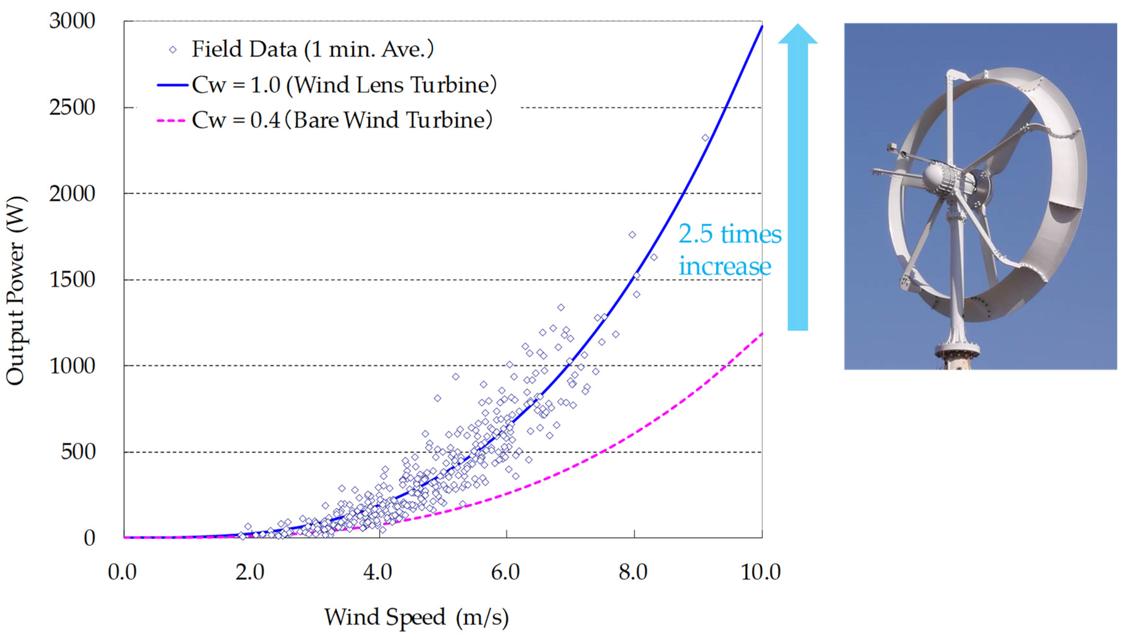
2. High Performance Wind Turbine Called Wind Lens Turbine (WLT)

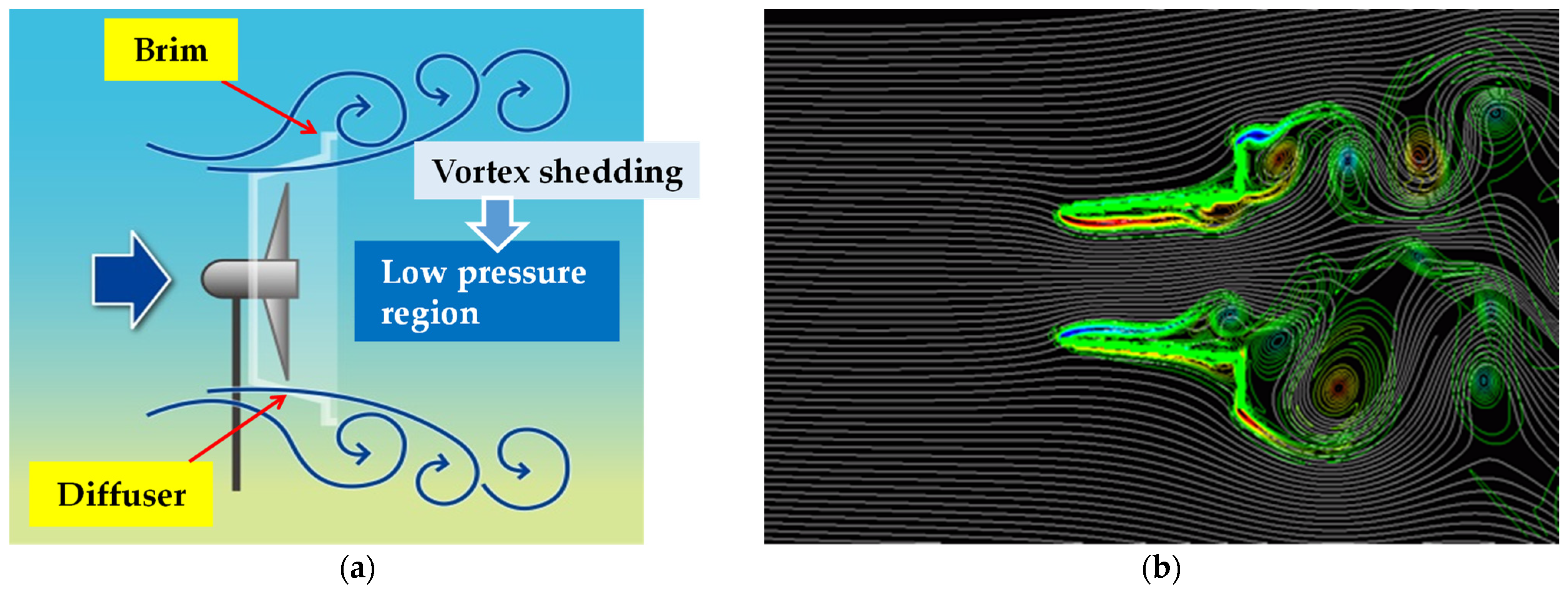
2.1. The Idea of a Shroud Diffuser with Brim

Wind power is proportional to the wind speed cubed. If wind speed can be increased with a mechanism by utilizing fluid dynamics around a structure, that is, if wind energy can be captured and concentrated locally, the output power of a wind turbine can be increased substantially [1,2,3,4,5,6,7,8]. There is potential for utilizing wind power in a more efficient way. In this study, the concept of accelerating the wind was named the “wind lens technology”, and the aim was to determine how to collect wind energy efficiently by using a simple structure called a wind lens [11,12,13].

For this purpose, we developed a diffuser-type structure that is capable of collecting and accelerating the approaching wind. As shown in Figure 1a, the diffuser shroud with the brim utilizes various flow characteristics of the flow inside or around it, such as the generation of low-pressure regions due to vortex formation and the entrainment of the flow by vortices. As a result, this shroud significantly increased the velocity of the approaching wind [11,12]. Although it adopts a diffuser-shaped structure surrounding a wind turbine like other ducted rotors [1,2,3,4,5,6,7,8,9,10], the feature that distinguishes it from the others is a large brim attached at the exit of the diffuser shroud. Figure 1b shows the two-dimensional flow around the wind lens structure illustrated by a direct numerical simulation using computational fluid dynamics (CFD). The convergence of the approaching flow into the diffuser is due to suction via strong vortex formation behind a brim. We actually placed a wind turbine inside a three-dimensional brimmed diffuser and measured its power output. The results showed that the brimmed diffuser wind turbine had power enhancement of about 2 to 5 times compared to a bare wind turbine of the same diameter (see Figure 2 and Figure 3). The augmentation ratio in power output mainly depends on the brim height, diffuser shape and length. The results of the parametric studies were summarized in the references [18,19]. In parallel with the development of the shroud structure, the turbine blade and its airfoil section were designed to achieve the best performance by configuring the blade and brimmed diffuser to obtain maximum aerodynamics. The development of the blades, which provide its maximum power output in a low tip speed ratio range, is described in Reference [13].

2.2. Special Features of a Wind Turbine with a Brimmed Diffuser

The important features of a shrouded wind turbine with a brimmed diffuser are as follows:

• Wind lens technology: Two to five-fold increase in output power compared to conventional wind turbines due to concentration of the wind energy (Figure 2 and Figure 3). The power output increase mainly depends on the diffuser shape and length and the brim height [11,12].
• Brim-based yaw control: The brim at the exit of the shroud makes a wind turbine rotate following a change in wind direction, similar to a weathervane. As a result, the wind turbine automatically turns to face the wind.
• Significant reduction in wind turbine noise, as shown in Figure 4. An airfoil section of the turbine blade is chosen that gives the best performance in a low tip speed ratio range. Since the vortices generated from the blade tips are considerably suppressed via interference with the boundary layer developed along the inside of the shroud, aerodynamic noise is reduced substantially [14,15].
• Improved safety: The wind turbine, rotating at a high speed, is shrouded by a structure and is also protected from damage from broken blades.
• Clustering of the shrouded wind turbines increases the power output of each wind turbine. This is the synergistic effect due to the accelerated gap flows between the brims [21,22].
• As for demerits, the wind load to a wind turbine and structural weight are increased.

This wind lens technology is also applicable to water turbines. We recently showed similar improvements in efficiency using a prototype of a water lens turbine using a water tunnel and computational fluid dynamics (CFD) [23,24].

3. One-Dimensional Simple Theory

3.1. Definition of Dimensionless Coefficients Related to the Wind Turbine Performance

In this section, we first define the dimensionless coefficients necessary for the following discussion. In this paper, we assume that the wind flows one-dimensionally. The air pressure, p, and x-direction (streamwise) wind speed, u, in front of and behind the wind turbine are indicated by Indices 1 and 2, respectively, as shown in Figure 5. The flow rate through the wind turbine is set to Q, air density is set to ρ, and flow loss is set to $\widetilde{{\mathrm{p}}_{\mathrm{t}}}$. This flow loss is the viscous loss of dynamic pressure of the flow at around the turbine, expressed in the dimension of pressure. Then, the energy equations in front of and behind the wind turbine show that the power output W of the wind turbine is

$$\mathrm{W}=\mathrm{Q}\left[\left({\mathrm{p}}_1+\frac{1}{2}{\mathsf{\rho }\mathrm{u}}_1{}^2\right)-\left({\mathrm{p}}_2+\frac{1}{2}{\mathsf{\rho }\mathrm{u}}_2{}^2\right)-\widetilde{{\mathrm{p}}_{\mathrm{t}}}\right]=\left({\mathrm{p}}_1-{\mathrm{p}}_2\right)\mathrm{Q}-\frac{1}{2}\mathsf{\rho }\mathrm{Q}\left({\mathrm{u}}_2{}^2-{\mathrm{u}}_1{}^2\right)-\widetilde{{\mathrm{p}}_{\mathrm{t}}}\mathrm{Q},$$

(1)

In the most right-hand side of the above equation, the first term is the input power, the second term is the energy loss due to the rotation of outlet flow, and the third term is the energy loss due to the pressure loss. The wind turbine efficiency, ${\mathsf{\eta }}_{\mathrm{T}}$, of the wind turbine is expressed by

$${\mathsf{\eta }}_{\mathrm{T}}=\frac{\mathrm{W}}{\left({\mathrm{p}}_1-{\mathrm{p}}_2\right)\mathrm{Q}}=1-\frac{\mathsf{\rho }\left({\mathrm{u}}_2{}^2-{\mathrm{u}}_1{}^2\right)/2+\widetilde{{\mathrm{p}}_{\mathrm{t}}}}{\left({\mathrm{p}}_1-{\mathrm{p}}_2\right)},$$

(2)

Ideally, the energy that the fluid loses by working on the wind turbine is equal to the energy that the wind turbine extracts from the fluid. However, in practice, the two are not equal because of the losses. ${\mathsf{\eta }}_{\mathrm{T}}$ shows the ratio of them. Normally, for the power coefficients of the wind turbine, the input power coefficient C_p corresponding to the denominator in Equation (2) is made dimensionless by using the upstream wind speed U₀ and the area of incoming airflow A. Similarly, the output power coefficient C_w, corresponding to the numerator in Equation (2), is made dimensionless as follows.

$${\mathrm{C}}_{\mathrm{P}}=\frac{\left({\mathrm{p}}_1-{\mathrm{p}}_2\right)\mathrm{Q}}{{\mathsf{\rho }\mathrm{U}}_0{}^3\mathrm{A}/2},$$

(3)

$${\mathrm{C}}_{\mathrm{W}}=\frac{\mathrm{W}}{{\mathsf{\rho }\mathrm{U}}_0{}^3\mathrm{A}/2}={\mathsf{\eta }}_{\mathrm{T}}{\mathrm{C}}_{\mathrm{P}},$$

(4)

The output power coefficient C_w takes into account the wind turbine loss and is always smaller than C_p.

In addition, as for the dimensionless forms of input and output powers, this paper defines the load and work coefficients for input and output based on the inflow velocity u₁ just before the wind turbine and the net wind area excluding the hub. In other words, the hub ratio (hub diameter/rotor diameter) is set to ν, and the inflow velocity ratio K is set to

$$\mathrm{K}={\mathrm{u}}_1/{\mathrm{U}}_0,$$

(5)

Then, the load coefficient Ψ and work coefficient Φ are expressed as follows:

$$\mathsf{\Psi }=\frac{\left({\mathrm{p}}_1-{\mathrm{p}}_2\right)\mathrm{Q}}{{\mathsf{\rho }\mathrm{u}}_1{}^3\mathrm{A}\left(1-{\mathsf{\nu }}^2\right)/2}=\frac{{\mathrm{p}}_1-{\mathrm{p}}_2}{{\mathsf{\rho }\mathrm{u}}_1{}^2/2}=\frac{{\mathrm{C}}_{\mathrm{P}}}{{\mathrm{K}}^3\left(1-{\mathsf{\nu }}^2\right)},$$

(6)

$$\mathsf{\Phi }=\frac{\mathrm{W}}{{\mathsf{\rho }\mathrm{u}}_1{}^3\mathrm{A}\left(1-{\mathsf{\nu }}^2\right)/2}=\frac{{\mathrm{C}}_{\mathrm{W}}}{{\mathrm{K}}^3\left(1-{\mathsf{\nu }}^2\right)}={\mathsf{\eta }}_{\mathrm{T}}\mathsf{\Psi },$$

(7)

The load coefficient Ψ represents the ratio of the extracted energy from the fluid working on the turbine compared to the kinetic energy of the inflow. The work coefficient Φ represents the ratio of the output energy from the turbine compared to the kinetic energy of the inflow.

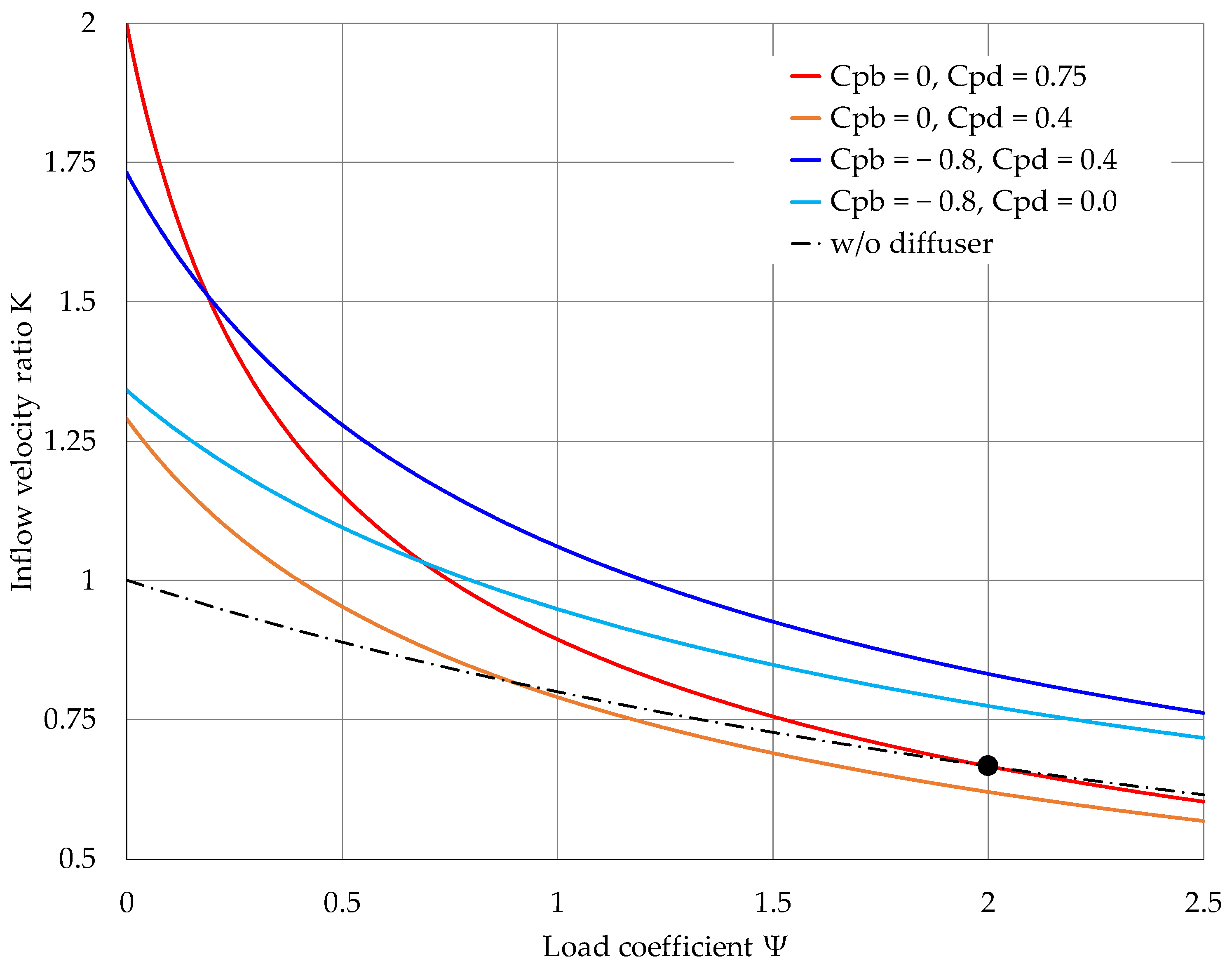
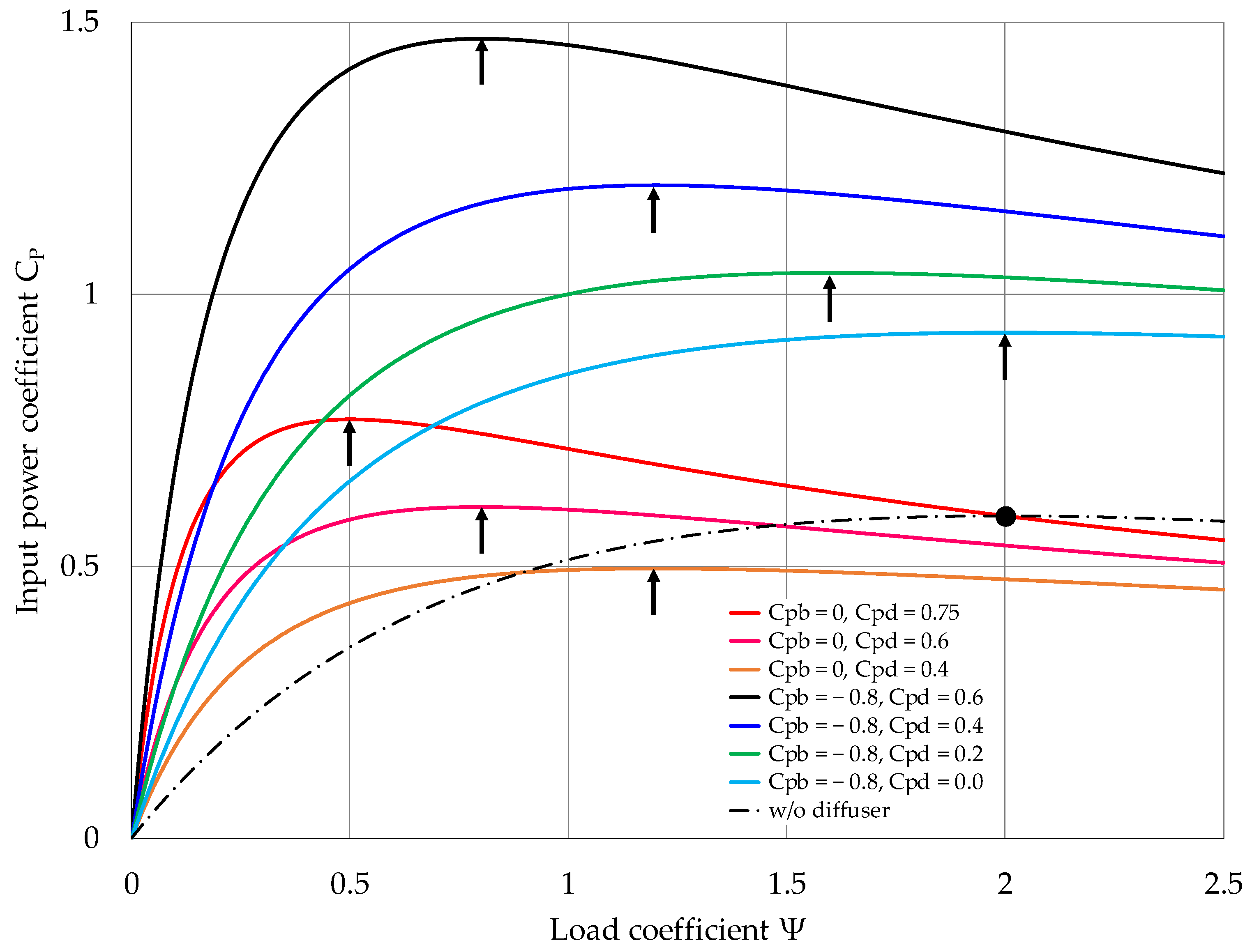
3.2. Performance Characteristics of the Brimmed Diffuser Augmented Wind Turbine

Here we theoretically derive the maximum power coefficient of a shrouded wind turbine with a brimmed diffuser. In the following discussion, we suggest the importance of considering the back pressure of a brim.

As shown in Figure 5, when a wind turbine is placed in the brimmed diffuser, the back pressure p_b behind the brim is lower than the atmospheric pressure p_a, and the pressure inside the diffuser is recovered from the pressure p₂ immediately behind the wind turbine to the back pressure p_b. Then the pressure outside the diffuser is recovered from the back pressure p_b to the atmospheric pressure p_a by mixing the low-speed fluid passing through the wind turbine with the high-speed fluid outside. Therefore, the back pressure coefficient of the brim C_pb and the pressure recovery coefficient of the diffuser C_pd are defined, respectively, as follows:

$${\mathrm{p}}_{\mathrm{a}}-{\mathrm{p}}_1=\frac{1}{2}\mathsf{\rho }\left({\mathrm{u}}_1{}^2-{\mathrm{U}}_0{}^2\right)=\frac{1}{2}{\mathsf{\rho }\mathrm{U}}_0{}^2\left({\mathrm{K}}^2-1\right),$$

(8)

$${\mathrm{p}}_{\mathrm{b}}-{\mathrm{p}}_2=\frac{1}{2}{\mathsf{\rho }\mathrm{C}}_{\mathrm{pd}}{\mathrm{u}}_1{}^2=\frac{1}{2}{\mathsf{\rho }\mathrm{C}}_{\mathrm{pd}}{\mathrm{K}}^2{\mathrm{U}}_0{}^2,$$

(9)

$${\mathrm{p}}_{\mathrm{b}}-{\mathrm{p}}_{\mathrm{a}}=\frac{1}{2}{\mathsf{\rho }\mathrm{C}}_{\mathrm{pb}}{\mathrm{U}}_0{}^2\left({\mathrm{C}}_{\mathrm{pb}}<0\right),$$

(10)

In Equation (8), the inlet loss was disregarded. The effect of the pressure loss in the diffuser and around the brim is included in the values of C_pd and C_pb, respectively. The pressure difference between the front and rear of the wind turbine shown in Equations (8)–(10) is as follows:

$${\mathrm{p}}_1-{\mathrm{p}}_2=\frac{1}{2}{\mathsf{\rho }\mathrm{U}}_0{}^2\left[1-{\mathrm{C}}_{\mathrm{pb}}-{\mathrm{K}}^2\left(1-{\mathrm{C}}_{\mathrm{pd}}\right)\right],$$

(11)

According to the above equation and Equations (5) and (6),

$$\mathrm{K}=\sqrt{\frac{1-{\mathrm{C}}_{\mathrm{pb}}}{1-{\mathrm{C}}_{\mathrm{pd}}+\mathsf{\Psi }}}$$

(12)

$$\frac{{\mathrm{C}}_{\mathrm{P}}}{1-{\mathsf{\nu }}^2}={\mathsf{\Psi }\mathrm{K}}^3=\mathsf{\Psi }{\left[\frac{1-{\mathrm{C}}_{\mathrm{pb}}}{1-{\mathrm{C}}_{\mathrm{pd}}+\mathsf{\Psi }}\right]}^{3/2},$$

(13)

In the following part of this section, we mention only C_p as a turbine performance indicator, but the analogous discussion can be applied to C_w.

Figure 6 shows the effects of the back pressure coefficient C_pb and pressure recovery coefficient C_pd on the inflow velocity ratio K. The dashed line in the figure is the value of K based on Betz’s theory (see Appendix A) of the ideal wind turbine without a brimmed diffuser, and ● in the figure corresponds to the limit condition of the power coefficient in Betz’s theory. For a diffuser without a brim, (C_pb = 0.0); if the load coefficient Ψ increases, the inflow velocity ratio decreases significantly, and at Ψ = 2, the acceleration effect cannot be increased beyond the limit condition of Betz, unless the pressure recovery coefficient of the diffuser is set to C_pd > 0.75. However, when C_pb = −0.8 and even when C_pd = 0.0, the inflow velocity ratio K is expected to be larger than the limit condition of Betz.

Figure 7 shows the effect of the diffuser and brim on the input coefficients, and for comparison, the values based on Betz’s theory of the wind turbine alone are shown by the single-dotted chain and ●. With a brimless diffuser (C_pb = 0.0), if the load coefficient Ψ of the wind turbine is not small, Betz’s power coefficient cannot be exceeded. However, for C_pb = −0.8, even if C_pd is zero, a larger input coefficient C_P than Betz’s theoretical value can be expected. Assuming that C_pb and C_pd do not vary with the load coefficient Ψ of the wind turbine, the maximum value of the input coefficient C_P is given by the following equation:

$$\frac{{\mathrm{C}}_{\mathrm{P},\max }}{1-{\mathsf{\nu }}^2}=\sqrt{\frac{4{\left(1-{\mathrm{C}}_{\mathrm{pb}}\right)}^3}{27\left(1-{\mathrm{C}}_{\mathrm{pd}}\right)}}=0.3849\sqrt{\frac{{\left(1-{\mathrm{C}}_{\mathrm{pb}}\right)}^3}{1-{\mathrm{C}}_{\mathrm{pd}}}},$$

(14)

Here,

$${\mathsf{\Psi }}_{{\mathrm{C}}_{\mathrm{P},\max }}=2\left(1-{\mathrm{C}}_{\mathrm{pd}}\right),$$

(15)

$${\mathrm{K}}_{{\mathrm{C}}_{\mathrm{P},\max }}=\sqrt{\frac{1-{\mathrm{C}}_{\mathrm{pb}}}{3\left(1-{\mathrm{C}}_{\mathrm{pd}}\right)}},$$

(16)

Equation (15) is derived by setting $\partial {\mathrm{C}}_{\mathrm{P}}/\partial \mathsf{\Psi }=0$ with differentiating Equation (13). By substituting Equation (15) into Equations (12) and (13), we derive Equations (14) and (16). The load coefficient Ψ with the maximum input coefficient C_P becomes smaller, as the pressure recovery coefficient C_pd becomes larger, but it is independent of the back pressure coefficient C_pb of the brim (see the arrow in Figure 7).

Figure 8 shows a line diagram for determining the maximum input coefficient C_P when the back pressure coefficient C_pb and the pressure recovery coefficient C_pd are known. The straight line shown by a dotted line shows the corresponding inflow velocity ratio K. The single point chain is the line corresponding to Betz’s limit conditions C_P,max = 16/27 and ${\mathrm{K}}_{{\mathrm{c}}_{\mathrm{P}},\max }$ = 2/3. In the upper right region from the single point chain line, the input coefficient C_P is larger than Betz’s limit value, indicating that there is a flow collection effect (wind lens effect). That is, the condition where the maximum input power coefficient C_p,max is larger than Betz’s limit condition C_p,max = 16/27 = 0.593 and ${\mathrm{K}}_{{\mathrm{c}}_{\mathrm{P}},\max }$ = 2/3 is calculated using the following equation:

$$\frac{{\left(1-{\mathrm{C}}_{\mathrm{pb}}\right)}^3}{1-{\mathrm{C}}_{\mathrm{pd}}}>{\left(\frac{4}{3}\right)}^3\cong 2.37,$$

(17)

3.3. Evaluation of One-Dimensional Simple Theory for Wind Lens Turbines

In this section, we validate our simple theory by comparing the theoretical values with experimental results. We used experimental results of three WLT models to validate the theory. The first model was a wind lens turbine with a long diffuser and large brim, as shown in Figure 9a. This WLT has the highest power increase rate ever developed. The second WLT called “Sii” shown in Figure 9b had a short diffuser with a semi-open angle of 12° and a short brim. The WLT called “Bii”, shown in Figure 9c, had a short diffuser with a gradually increasing opening angle and a short brim. These two compact WLTs are practical because of their light weight and small wind loads. The NACA (National Advisory Committee for Aeronautics) airfoil blades were used for the long type WLT. For the compact type WLTs, MEL (Mechanical Engineering Laboratory) airfoil blades were used. All turbines had three blades.

Experiments were conducted in the wind tunnel at RIAM, Kyushu University. The turbulence intensity of the approaching wind was less than 0.5%. The effect of Reynolds number on the power output of the wind turbine was checked in advance, and the approaching wind speed was set to 8 m/s. The power output of the wind turbine W was calculated as the product of the torque measured by a torque transducer and the angular velocity of the blade rotation. The rotation speed of the wind turbine was controlled by an AC servomotor. The wind velocity u₁ distributions in the radial direction in front of the rotating plane of blades were measured at each optimal tip speed ratio using an I-type hot-wire with an anemometry. At the same time, the radial distribution of pressure difference in front of the rotating surface of the blade (p₁–p_a), behind the rotor (p₂–p_a), and at diffuser outlet (p_b–p_a) were also measured using a static pressure tube with a manometer. The pressure coefficient in front of the wind turbine is defined as ${\mathrm{C}}_{\mathrm{p}1}=\left({\mathrm{p}}_1-{\mathrm{p}}_{\mathrm{a}}\right)/\left(\frac{1}{2}{\mathsf{\rho }\mathrm{U}}_0{}^2\right)$, and coefficient behind the wind turbine is defined as ${\mathrm{C}}_{\mathrm{p}2}=\left({\mathrm{p}}_2-{\mathrm{p}}_{\mathrm{a}}\right)/\left(\frac{1}{2}{\mathsf{\rho }\mathrm{U}}_0{}^2\right)$. The performance coefficients were calculated experimentally and theoretically by the equations listed in

Table 1. Equations for calculating the performance coefficients.

Coefficients	Experiment	Simple Theory
Back pressure coefficient, Cpb	${\mathrm{C}}_{\mathrm{pb}} \left(=\frac{{\mathrm{p}}_{\mathrm{b}}-{\mathrm{p}}_{\mathrm{a}}}{\frac{1}{2}{\mathsf{\rho }\mathrm{U}}_0{}^2}\right)$	(use experimental value)
Pressure recovery coefficient, Cpd	$\frac{{\mathrm{C}}_{\mathrm{pb}}-{\mathrm{C}}_{\mathrm{p}2}}{{\mathrm{K}}^2}$	(use experimental value)
Inflow velocity ratio, ${\mathrm{K}}_{{\mathrm{C}}_{\mathrm{P},\max }}$	$\mathrm{K}\left(=\frac{{\mathrm{u}}_1}{{\mathrm{U}}_0}\right)$	$\sqrt{\frac{1-{\mathrm{C}}_{\mathrm{pb}}}{3\left(1-{\mathrm{C}}_{\mathrm{pd}}\right)}}$
Load coefficient, ${\mathsf{\Psi }}_{{\mathrm{C}}_{\mathrm{P},\max }}$	$\frac{{\mathrm{C}}_{\mathrm{p}1}-{\mathrm{C}}_{\mathrm{p}2}}{{\mathrm{K}}^2}$	$2\left(1-{\mathrm{C}}_{\mathrm{pd}}\right)$
Maximum input power coefficient, CP,max	$\left({\mathrm{C}}_{\mathrm{p}1}-{\mathrm{C}}_{\mathrm{p}2}\right)\left(1-{\nu }^2\right)\mathrm{K}$	$\left(1-{\nu }^2\right)\sqrt{\frac{4{\left(1-{\mathrm{C}}_{\mathrm{pb}}\right)}^3}{27\left(1-{\mathrm{C}}_{\mathrm{pd}}\right)}}$

.

For a wind lens turbine with a long diffuser and large brim, as shown in Figure 9a, we obtained power curves (Figure 10) and the values of inflow velocity ratio K, back pressure coefficient C_pb, and pressure coefficients C_p1, C_p2 in wind tunnel experiments, as shown in Figure 12. This long WLT produced the largest C_w and K values among the three types of WLTs, and the lowest C_p2 was achieved due to the large pressure change inside the diffuser. For compact wind lens turbines, we obtained power curves (Figure 11), and values of K, C_pb, C_p1 and C_p2 in wind tunnel experiments, as shown in Figure 12. A clear difference in the maximum value of C_w was observed although the shroud shapes of the two WLTs were not significantly different. The C_pb and C_p2 values of Bii-type WLT were clearly lower than those of Sii-type WLT near the blade tip, while there was no significant difference in the value of K. The radial distributions of the pressure were not negligible for the compact WLTs. Therefore, we curve-fitted all quantity distributions with a linear function and calculated the average value of the performance coefficients by integrating them along the radial direction.

All the calculated coefficients are shown in

Table 2. Comparison of various coefficients between experiments and predictions by the simple theory at C_P,max (at λ = 4.5) for a wind turbine with the long diffuser and large brim shown in Figure 9a.

Parameters	Experiment Averaged Values by Wind Tunnel Experiments at CP,max	Simple Theory Estimated Values by The Simple Theory at CP,max
Back pressure coefficient, Cpb	−0.55 (from Figure 12b)	(−0.55; experimental result)
Pressure recovery coefficient, Cpd	0.55 (from Figure 12b)	(0.55; experimental result)
Inflow velocity ratio, ${\mathrm{K}}_{{\mathrm{C}}_{\mathrm{P},\max }}$	1.2 (from Figure 12a)	1.1
Load coefficient, ${\mathsf{\Psi }}_{{\mathrm{C}}_{\mathrm{P},\max }}$	0.76	0.90
Maximum input power coefficient, CP,max	1.3	1.1
Wind turbine efficiency, ${\mathsf{\eta }}_{\mathrm{T}}\left(={\mathrm{C}}_{\mathrm{W}}/{\mathrm{C}}_{\mathrm{P}}\right)$	1.0	-

,

Table 3. Comparison of various coefficients between experiments and predictions by the simple theory at C_P,max (at λ = 4.0) for a wind turbine with the compact Sii brimmed diffuser shown in Figure 9b.

Parameters	Experiment Averaged Values by Wind Tunnel Experiments at CP,max	Simple Theory Estimated Values by The Simple Theory at CP,max
Back pressure coefficient, Cpb	−0.83 (from Figure 12c)	(−0.83; experimental result)
Pressure recovery coefficient, Cpd	0.22 (from Figure 12c)	(0.22; experimental result)
Inflow velocity ratio, ${\mathrm{K}}_{{\mathrm{C}}_{\mathrm{P},\max }}$	0.86 (from Figure 12a)	0.89
Load coefficient, ${\mathsf{\Psi }}_{{\mathrm{C}}_{\mathrm{P},\max }}$	1.6	1.6
Maximum input power coefficient, CP,max	1.0	1.0
Wind turbine efficiency, ${\mathsf{\eta }}_{\mathrm{T}}\left(={\mathrm{C}}_{\mathrm{W}}/{\mathrm{C}}_{\mathrm{P}}\right)$	0.71	-

and

Table 4. Comparison of various coefficients between experiments and predictions by the simple theory at C_P,max (at λ = 4.0) for a wind turbine with the compact Bii brimmed diffuser shown in Figure 9c.

Parameters	Experiment Averaged Values by Wind Tunnel Experiments at CP,max	Simple Theory Estimated Values by The Simple Theory at CP,max
Back pressure coefficient, Cpb	−0.97 (from Figure 12d)	(−0.97; experimental result)
Pressure recovery coefficient, Cpd	0.28 (from Figure 12d)	(0.28; experimental result)
Inflow velocity ratio, ${\mathrm{K}}_{{\mathrm{C}}_{\mathrm{P},\max }}$	0.91 (from Figure 12a)	0.97
Load coefficient, ${\mathsf{\Psi }}_{{\mathrm{C}}_{\mathrm{P},\max }}$	1.6	1.4
Maximum input power coefficient, CP,max	1.2	1.2
Wind turbine efficiency, ${\mathsf{\eta }}_{\mathrm{T}}\left(={\mathrm{C}}_{\mathrm{W}}/{\mathrm{C}}_{\mathrm{P}}\right)$	0.72	-

. The experimental values and predicted values by the simple theory were close to each other. For the long type WLT, the prediction was slightly less accurate. We attributed this to measurement error in the experiment, due to the long inlet of the WLT, which made it difficult to set up a measurement device upstream of the wind turbine. The existence of measurement errors in the experimental results was also suggested by the too large wind turbine efficiency of ${\mathsf{\eta }}_{\mathrm{T}}=1.0$. Experimental results with good accuracy will give more accurate theoretical predictions. For the compact WLTs, the values of ${\mathsf{\eta }}_{\mathrm{T}}$ was reasonable, and the performance difference between the two compact WLTs (Sii and Bii) was estimated with good accuracy. Hence, we would like to propose this simplified theory as a method to give a good estimation. The critical implication of this theory is that the output coefficient depends only on the magnitude of Cpb and Cpd. To have a higher output power coefficient Cw, the brimmed diffuser should have a lower back pressure coefficient C_pb and a higher pressure recovery coefficient C_pd especially near the tip of the blade.

4. Conclusions

We developed a new wind turbine system that consists of a diffuser shroud with a brim at the outlet and a wind turbine inside it. The shrouded wind turbine with a brimmed diffuser, which we called a “wind lens turbine” (WLT), has demonstrated power augmentation by a factor of about 2–5 compared with a bare wind turbine, for a given turbine diameter and wind speed. The augmentation ratio in power output depends on the diffuser length, brim height, and the turbine’s configurations. However, by constructing a one-dimensional theory of WLT, we showed that its performance depended only on the values of two important performance coefficients, the back pressure coefficient of the brim and the pressure recovery coefficient of the diffuser. Theoretically, the following results were derived:

⮚

DAWTs are not able to achieve output beyond Betz’s limit unless the pressure behind it is lower than the reference pressure upstream.

⮚

If the pressure behind the DAWT is lower than the upstream reference pressure, the DAWT is able to achieve output beyond Betz’s limit without the effect of the diffuser.

The above results show the importance of reducing the pressure behind the DAWT. The WLT is an efficient wind turbine that reduces the pressure behind itself by the brim.

We applied the presented simple theory to both wind turbines with a compact brimmed diffuser and a wind turbine with a long diffuser and large brim. As the results show, the simple theory can give a good estimation of the maximum power output. Multiple stream tube theory would be welcomed to deal with variations of physical quantities in the radial direction of the wind turbine.

References

1. Gilbert, B.L.; Oman, R.A.; Foreman, K.M. Fluid dynamics of diffuser-augmented wind turbines. J. Energy 1978, 2, 368–374. [Google Scholar] [CrossRef]
2. Gilbert, B.L.; Foreman, K.M. Experiments with a Diffuser-Augmented Model Wind Turbine. J. Energy Resour. Technol. 1983, 105, 46–53. [Google Scholar] [CrossRef]
3. Hansen, M.O.L.; Sørensen, N.N.; Flay, R.G.J. Effect of Placing a Diffuser around a Wind Turbine. Wind Energy 2000, 3, 207–213. [Google Scholar] [CrossRef]
4. Sedaghat, A.; Al Waked, R.; El Haj, A.M.; Khanafer, K.; Salim, M.N.B. Analysis of Accelerating Devices for Enclosure Wind Turbines. Int. J. Astronaut. Aeronaut. Eng. 2017, 2, 009. [Google Scholar] [CrossRef] [Green Version]
5. Khamlaj, T.A.; Rumpfkeil, M.P. Analysis and optimization of ducted wind turbines. Energy 2018, 162, 1234–1252. [Google Scholar] [CrossRef]
6. Nunes, M.M.; Junior, A.C.P.B.; Oliveira, T.F. Systematic review of diffuser-augmented horizontal-axis turbines. Renew. Sustain. Energy Rev. 2020, 133, 110075. [Google Scholar] [CrossRef]
7. Van Bussel, G.J.W. The science of making more torque from wind: Diffuser experiments and theory revisited. J. Physics Conf. Ser. 2007, 75, 012010. [Google Scholar] [CrossRef]
8. Jamieson, P. Innovation in Wind Turbine Design, 2nd ed.; John Wiley & Sons Ltd.: Hoboken, NJ, USA, 2011; pp. 13–63. [Google Scholar]
9. Freda, R.; Knight, B.; Pannir, S. A Theory for Power Extraction from Passive Accelerators and Confined Flows. Energies 2020, 13, 4854. [Google Scholar] [CrossRef]
10. Bontempo, R.; Manna, M. Diffuser augmented wind turbines: Review and assessment of theoretical models. Appl. Energy 2020, 280, 115867. [Google Scholar] [CrossRef]
11. Abe, K.; Nishida, M.; Sakurai, A.; Ohya, Y.; Kihara, H.; Wada, E.; Sato, K. Experimental and numerical investigations of flow fields behind a small wind turbine with a flanged diffuser. J. Wind Eng. Ind. Aerodyn. 2005, 93, 951–970. [Google Scholar] [CrossRef]
12. Ohya, Y.; Karasudani, T. A Shrouded Wind Turbine Generating High Output Power with Wind-lens Technology. Energies 2010, 3, 634–649. [Google Scholar] [CrossRef] [Green Version]
13. Oka, N.; Furukawa, M.; Kawamitsu, K.; Yamada, K. Optimum aerodynamic design for wind-lens turbine. J. Fluid Sci. Technol. 2016, 11, JFST0011. [Google Scholar] [CrossRef] [Green Version]
14. Abe, K.; Kihara, H.; Sakurai, A.; Wada, E.; Sato, K.; Nishida, M.; Ohya, Y. An experimental study of tip-vortex structures behind a small wind turbine with a flanged diffuser. Wind Struct. 2006, 9, 413–417. [Google Scholar] [CrossRef]
15. Takahashi, S.; Hata, Y.; Ohya, Y.; Karasudani, T.; Uchida, T. Behavior of the Blade Tip Vortices of a Wind Turbine Equipped with a Brimmed-Diffuser Shroud. Energies 2012, 5, 5229–5242. [Google Scholar] [CrossRef] [Green Version]
16. Watanabe, K.; Ohya, Y.; Uchida, T. Power Output Enhancement of a Ducted Wind Turbine by Stabilizing Vortices around the Duct. Energies 2019, 12, 3171. [Google Scholar] [CrossRef] [Green Version]
17. Betz, A. The Maximum of the Theoretically Possible Exploitation of Wind by Means of a Wind Motor. Wind Eng. 2013, 37, 441–446. [Google Scholar] [CrossRef]
18. Ohya, Y.; Karasudani, T.; Sakurai, A.; Inoue, M. Development of a High-Performance Wind Turbine Equipped with a Brimmed Diffuser Shroud. Trans. Jpn. Soc. Aeronaut. Space Sci. 2006, 49, 18–24. [Google Scholar] [CrossRef] [Green Version]
19. Ohya, Y.; Karasudani, T.; Sakurai, A.; Inoue, M. Development of High-Performance Wind Turbine with a Brimmed-Diffuser—Part 2. J. Jpn. Soc. Aeronaut. Space Sci. 2004, 52, 210–213. (In Japanese) [Google Scholar] [CrossRef] [Green Version]
20. Introduction of RIAMWIND Co., Ltd. Available online: riamwind.co.jp/English/introduction.html (accessed on 18 June 2021).
21. Yuji, O.; Koichi, W.; Ohya, Y.; Watanabe, K. A New Approach Toward Power Output Enhancement Using Multirotor Systems with Shrouded Wind Turbines. J. Energy Resour. Technol. 2019, 141, 051203. [Google Scholar] [CrossRef] [Green Version]
22. Watanabe, K.; Ohya, Y. Multirotor Systems Using Three Shrouded Wind Turbines for Power Output Increase. J. Energy Resour. Technol. 2019, 141, 141. [Google Scholar] [CrossRef] [Green Version]
23. Sun, H.; Kyozuka, Y. Analysis of performances of a shrouded horizontal axis tidal turbine. In Proceedings of the 2012 Oceans—Yeosu, Yeosu, Korea, 21–24 May 2012; Institute of Electrical and Electronics Engineers (IEEE): Piscataway, NJ, USA, 2012. [Google Scholar] [CrossRef]
24. Watanabe, K.; Ohya, Y. Water Turbines with a Brimmed Diffuser By using Wind Lens Technology. Int. J. Energy Clean Environ. 2021, 22, 33–45. [Google Scholar] [CrossRef]
Figure 1. (a) Mechanism of wind lens technology. Adapted from ref. [20]; (b) two-dimensional flow around a wind lens using computational fluid dynamics (CFD). The white lines show streamlines, and flow is accelerated where the lines are closely spaced. The multi-colored lines are vorticity contours, where blue represents clockwise vorticity and red represents counterclockwise vorticity.
Energies 14 03661 g001
Figure 2. Field experiment of a 500 W wind lens turbine (WLT) with a long brimmed diffuser, a rotor diameter of 0.7 m, and a lens diameter of 1.8 m.
Energies 14 03661 g002
Figure 3. Field experiment of a 3 kW wind lens turbine (WLT) with a compact brimmed diffuser, a rotor diameter of 2.5 m, and a lens diameter of 3.2 m. Adapted from ref. [20].
Energies 14 03661 g003
Figure 4. Field experiment of a 100 kW wind lens turbine (WLT) with a rotor diameter of 12.8 m and a lens diameter of 15.4 m. Adapted from ref. [20].
Energies 14 03661 g004
Figure 5. Configuration of wind turbine with brimmed diffuser.
Energies 14 03661 g005
Figure 6. Variation of inlet velocity ratio K with loading coefficient.
Energies 14 03661 g006
Figure 7. Variation of input power coefficient with loading coefficient.
Energies 14 03661 g007
Figure 8. Maximum input power coefficient and inlet velocity ratio for a given combination of diffuser pressure-recovery coefficient and brim back pressure coefficient.
Energies 14 03661 g008
Figure 9. Configuration of the WLT models used in the experiment: (a) long type corresponds to the brimmed diffuser shown in Figure 2; (b) Sii refers to a straight diffuser with a brim and an open angle of 12 degrees; (c) Bii corresponds to the compact brimmed diffuser shown in Figure 3.
Energies 14 03661 g009
Figure 10. Power curves vs. λ (tip speed ratio) for a wind turbine with long diffuser and large brim and bare turbine. Cw is the output power coefficient.
Energies 14 03661 g010
Figure 11. Power curves vs. λ (tip speed ratio) for a wind turbine with compact brimmed diffusers of Sii, Bii and a bare turbine. Cw is the output power coefficient.
Energies 14 03661 g011
Figure 12. Coefficients measured in wind tunnel experiments: (a) inflow velocity ratio K; (b) pressure coefficients for the long brimmed diffuser; (c) pressure coefficients for Sii brimmed diffuser; (d) pressure coefficients for Bii brimmed diffuser.
Energies 14 03661 g012aEnergies 14 03661 g012b