Article

Probability-Based Failure Evaluation for Power Measuring Equipment

1
College of Electrical and Information Engineering, Hunan University, Changsha 410082, China
2
Department of Electrical Engineering and Computer Science, University of Tennessee, Knoxville, TN 37996, USA
*
Authors to whom correspondence should be addressed.
Energies 2021, 14(12), 3632; https://doi.org/10.3390/en14123632
Submission received: 24 May 2021 / Revised: 6 June 2021 / Accepted: 9 June 2021 / Published: 18 June 2021

Abstract

:
Accurate reliability and residual life analysis is paramount during the designing of reliability requirements and rotation of power measuring equipment (PME). However, the sample dataset of failure is usually sparse and contains inevitable pollution data, which has an adverse effect on the reliability analysis. To tackle this issue, this paper first applies nonlinear regression to fuse the failure rate and environmental features of PME collected from various locations. Then, a novel binary hierarchical Bayesian probability method is proposed to model the failure trend and identify outliers, in which the outlier identification structure is embedded into hierarchical Bayesian. Integrating binary hierarchical Bayesian and the bagging method, a binary hierarchical Bayesian with bagging (BHBB) framework is further introduced to improve predictive performance in a small sample dataset by resampling. Last, the influence of typical environmental features, failure rate, and reliability are obtained by the BHBB under the real sample dataset from multiple typical locations. Experiments show that our framework has superior performance and interpretability comparing with other typical data-based approaches.

1. Introduction

The failure rate of power measuring equipment (PME), namely the probability of failure over a certain period of time, is an important index of reliability research [1]. Accurate evaluation and prediction of failure rate are of critical importance for instrument rotation, aiding in business decisions, and customer service [2]. Meanwhile, more and more intelligent measuring equipment are put into operation with the development of a smart grid [3]. For example, the number of electrical meters worldwide has tripled from 10.3 million in 2012 to 29.9 million in 2017 according to reports in [4]. Nevertheless, the accurate reliability prediction of PME still suffers from some unavoidable factors, especially under extreme environments. For example, the reliability data collected in the outside world usually contain noise and outliers. Different record staff or systems may record data in a biased manner due to uncontrolled sources or data, resulting in decreased accuracy [5]. Therefore, it is necessary to adopt an effective method to analyze the failure data from different perspectives.
In recent decades, numerous approaches to evaluate failure have been developed [6]. Generally, they can be classified into three categories [7]: (1) conventional methods based on system structure, (2) deterministic methods, and (3) probabilistic analysis methods. Among them, fault tree analysis (FTA) is one of the most commonly used conventional methods for failure analysis. For instance, a system-level electric filed exposure evaluation is proposed based on component-level data with a series-parallel fault tree system [8]. To deal with multiple value systems, the dynamic fault tree is developed to compensate for the shortcomings of FTA [9]. However, FTA is suitable for failure analysis of specific instrument structures, for which it is difficult to analyze the influence of external environmental features.
To avoid issues that arise by different environment features, a number of deterministic approaches are used to aggregate the failure data with multivariate in different geographical areas. Some recent researches aim to solve failure analysis, including partial least squares regression (PLSR) and encoding methods using neural network (NN) [10]. However, the NN method requires sufficient data learning parameters, since it belongs to the data-driven methods. Additionally, the prediction methods based on data mining, such as statistics method and support vector machine (SVM), are used for reliability and uncertainty assessment [11]. They enable the integration of external factors but lack the correlation in external factors and parameter interpretability.
Different from the deterministic methods, the probabilistic analysis method can be employed to treat the information on faults sharing across time and through space. Wiener degradation (WN) and Gaussian degradation (GP) are stochastic processes. They have been widely used for data-driven degradation. However, it needs to be emphasized that they are more suitable for accelerated life analysis. In [12], an accelerated degradation testing based on time-to-failure Weibull distribution is established to predict the reliability of the smart electricity meter. Some other acceleration methods can be found in the literature [13]. However, this reliability model is difficult to predict with actual environmental operational data.
To avoid isolation of features and models, different Bayesian models have been proposed to make evaluations and predicts of failure rate. The unique advantage of Bayesian is that it combines prior information and can provide confidence intervals [14]. Yuan and Kuo [15] developed a Bayesian approach to model the hazard rate with Weibull exponential distribution. Hierarchical Bayesian (HB), a multi-information fusion method, is suitable for the estimation of the individual or multiple variables [16]. Combined with the regression model, HB can also provide accurate fitting and probability prediction ability for the failure rate model [7]. Additionally, some other probabilistic approaches, e.g., the nonparametric Bayesian methods, can also be used for failure and reliability evaluation. Different types of failure data can be fused by the probabilistic analysis method [17]. Unfortunately, the Bayesian approach strongly relies on the accuracy of raw data. That is to say, the accuracy of HB is easily affected by the outliers and shortage of sample size [18]. Otherwise, a wide confidence interval and volatility forecast results will be provided. To resolve these difficulties and limitations mentioned above, a method for identifying outliers and being able to fuse multiple data is required.
The motivation of this paper is to enhance the failure evaluation performance of PME. The contributions of the proposed probability-based method are:
1.
To predict failure rate in different locations, a HB with nonlinear regression is proposed to integrate the environmental features and failure rate information of PME. The degree of influence of various environmental features can be then interpreted.
2.
To reduce the effect of outliers, a binary hierarchical Bayesian (BHB) is proposed to distinguish the outliers from the raw failure rate data. Particularly, the outlier identification term is embedded in a binary structure to simplify the data preprocessing process.
3.
Combined with the bagging method, a binary hierarchical Bayesian model with bagging (BHBB) is further proposed to reduce the failure prediction variance of the PME. The random resampling of BHBB avoids the weight assignment of samples without prior information compared with Bayesian bootstrap.
4.
Finally, the effectiveness of the proposed method is tested and verified with actual sample data of electricity meters from three typical locations. In addition, the relationship between failure rate and typical environmental features is then quantitatively analyzed.
The remainder of this paper is organized as follows: We begin by introducing the environmental characteristics and actual failure rate data in Section 2. Then, the proposed BHBB framework for outlier identification is developed in Section 3. Section 4 further explores the way to solve the proposed BHBB framework. In Section 5, different experiments are conducted to verify the effectiveness of the method. Finally, the conclusions are presented in Section 6.

2. The Environmental Features of PME

2.1. Environmental Features Analysis

To ensure accurate metering of PME, electric energy metering equipment is used as a data instance. It is reported that the State Grid Corporation of China has to check the status of meters every few years to ensure accurate and fair measurement [19]. Moreover, in the actual environment, the normal operation of the electrical meter is affected by various factors. In addition, it is difficult to eliminate the fault of the electrical meter one by one because of its wide distribution. Hence, the failure rate of the electrical meters can be analyzed to offer suggestions for providing trade-off decisions.
Obviously, the PME are more prone to failure under typical environmental stress. Therefore, the actual data collected from Xizang (XZ), Heilongjiang (HLJ), and Xinjiang (XJ) of China are used, which have extreme altitude, cold, and dryness, respectively. The relationship between the failure rate and typical environmental features is expected to be analyzed.
Table 1 summarizes the primary environmental features of the three locations. All environmental features are calculated using the annual average [20]. It can be seen from Table 1 that four primary features are considered, including the temperature, pressure, humidity, and illumination. Meanwhile, the average annual maximum temperature (M-Tem) and the average annual minimum temperature (N-Tem) are used to represent temperature characteristics. It shows that the most dramatic temperature change is in XJ. This means that the temperature difference in the area is relatively large. Furthermore, the humidity features are particularly high in XZ during the entire year. Conversely, the pressure is the smallest in XZ. The N-Tem of XJ is the lowest when the others have no obvious characteristics compared with XZ and HLJ. It is worth mentioning that multiple typical environmental features may also be superimposed on the PME at the same time. For example, there will be very high temperatures during the day in XJ.

2.2. Actual Failure Rate Sample of Electrical Meters

In this section, three real failure rate datasets of electrical meters from XZ, XJ, and HLJ provinces are used to illustrate the proposed method. The structure of the data acquisition system for electricity meters is shown in Figure 1. It shows that the operating state data of the electrical meters are transmitted to the concentrator through the power line. The operating state data mainly represent the electrical energy data, including current, voltage, power, and other measurement data when the meter is working. Then, the data of the concentrator is further transmitted by the base station through wireless transmission or power line. Finally, the data for number of failed meters of all locations is transferred to the server database. Moreover, if the meter fails to send the data for a certain time, its data loss state can be easily obtained and the meter may need to be replaced. As shown in Figure 1, the measuring unit mainly includes the three-phase electric energy meter and the single-phase electric energy meter. Meanwhile, the failure rate of the data includes LCD faults, out of tolerance, battery undervoltage, clock faults, and communication faults.
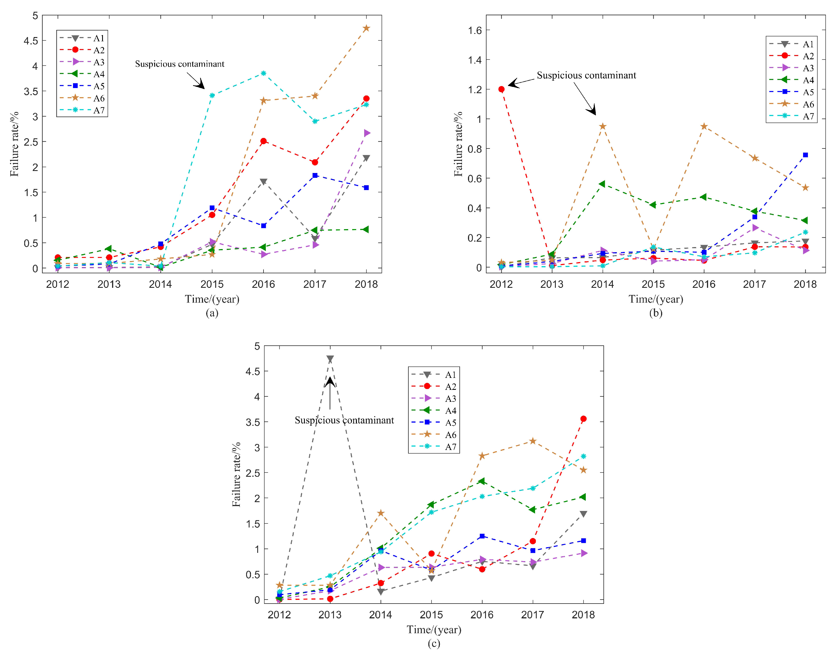
Figure 2 shows the failure rate data in three areas. All the data are collected from the same company to avoid the difference of objects between multiple areas. The datasets record 7 years of failure numbers from 2012 to 2018. Here, A1 to A7 is the abbreviation of the dataset, where each dataset contains 7 groups of subsets that collect from different areas in the same province, namely a total of 21 groups are obtained. The failure rate is calculated through failures recorded every year divided by the remaining electrical meters.
It can be seen from Figure 2 that the failure rate keeps growing during 2012–2016 and falls slightly in 2017. Obviously, the failure tendency has a strong correlation with time. The growth rates are also different from each other because the data are collected in different areas. Furthermore, several failure rate data points are particularly large in 2012–2016 of Figure 2b and 2013 in Figure 2c. Those values are completely different from other data. Therefore, it is reasonable to treat these points that are far from intensive data as suspected outliers.

3. Binary Hierarchical Bayesian with Bagging

3.1. Motivation

The hierarchical Bayesian framework allows users to build the model with multilayered probability distributions. It is more suitable for the analysis of small samples [16].
Let Y = X a , t , i , y a , t , i be the sample dataset where y a , t , i refers the ith failure rate data of PME in the area a at time t, X a , t , i refers the corresponding ith environmental features in area a at time t, and each X a , t , i is composed of different environmental features where a = 1 , 2 , 3 denotes three areas.
Generally, the failure rate can be specified to obey Weibull distribution. It is commonly used to describe electronic equipment failure [21], and the probability density function of Weibull distribution is
P w ( k α , β ) = β α ( k ) α 1 exp β k α
where α is the shape parameter, and β represents the scale parameter of Weibull distribution. k = y a , t , i denotes the failure rate, and α , β , and k are greater than 0. The change of the Weibull shape parameter usually indicates the failure mechanism changes. Thus, the Weibull shape parameter α remains constant while scale parameter β changes.
To integrate environmental features with temporal information, we establish a nonlinear regression based on the scale parameter β , which can be obtained as
log ( β ) = β 0 + β α , 1 t + + β α , q t q + β α , p X α , t , i + λ β α , p 2
where β 0 denotes the intercept when X a , t , i and t equal to zero, β α , p represent the pth slope in the linear equation, q = 1 , 2 , , n denotes the order of time t and p = q + 1 , , q + 4 ; λ β α , p 2 denotes regularization items to reduce overfitting. The log-scale log(·) is used to ensure the positive interval of parameter β . The order of polynomial depends on the balance between accuracy and the simplicity of the model.
The nonlinear regression Equation (2) combines all the effects and creates an underlying structure of the model. However, it cannot identify potential outliers, thus additional outlier identification structure is in great demand.

3.2. Proposed Binary Hierarchical Bayesian

Outliers can easily cause large deviations in small sample predictions. The traditional outlier detection methods, e.g., cluster-based and density-based, will fail in a small sample dataset [22]. However, deleting data points directly can easily lead to information loss.
In this paper, a binary hierarchical Bayesian is proposed to identify outliers. The binary method assumes each failure sample data was generated by a truly process being studied or by another outlier structure and, thus, a mixture likelihood is built to specify normal values and outliers. Formally, it extends the original model to include binary likelihood which consists of the Weibull and outlier assignments.
For a particular experiment, every element in Y believed to have been generated by two models, i.e., a truly Weibull parameter model p w parameterized by θ w , and another outlier model p c parameterized by θ c . Obviously, the binary parameter M = { m i } can be defined as follows: m i = 0 if ith data point was generated by the Weibull parameter model and m i = 1 if ith data point was generated by outlier model p c . Furthermore, the outlier model in binary hierarchical Bayesian model can be described as
y a , t , i P w · θ w , if m i = 0 p c · θ c , if m i = 1
where mi can be expressed as discrete distribution
m i Bernoulli ϕ i
where ϕ i is the probability of producing outliers for the stochastic process. Then, the likelihood of binary hierarchical Bayesian model is given as
L Y , M θ w , θ c , ϕ i = i = 1 N ϕ i m i 1 ϕ i 1 m i x 1 m i P w y a , i , t θ w + m i p c y a i t θ c
In practice, if the particular outlier is known, which means a known binary parameter M is obtained, the model can be inference via Markov chain Monte Carlo (MCMC) algorithm. However, sample collection staff rarely mark whether or not or which kind of data belongs in actual work, and some mistakes can then be made during the process.
Binary likelihood models data with a weight coefficient for different likelihoods. In our case of the model, the binary derives from marginalizing over the m i , and the likelihood can then be expressed as
L Y θ w , θ c , ϕ i = i = 1 N 1 ϕ i p w y a , t , i θ w + ϕ i p c y α , t , i θ c
After establishing binary hierarchical Bayesian, the inference can be performed using Bayesian updating or other schemes under this outlier likelihood. Alternatively, one can adopt no information prior to distribution Uniform(0, 1) for ϕ i . In the proposed method, we assign probit function ϕ ( · ) to ϕ i so that the binary structure can better fit the data due to the hierarchical structure. The probability density function of ϕ ( · ) is given by
ϕ i Φ ρ i = 1 2 + 1 2 erf ( ρ i / 2 )
where ρ i is the parameter of probit function ϕ ( · ) . When ϕ i = 1 , it represents the probability p c is generated by the outlier model. Thus, the prior distribution of p c , namely θ c , can be specified as Uniform(0, 1).

3.3. The Proposed BHBB Model

Failure mechanism performance is sensitive to small changes and can be easily disturbed in a small sample dataset. Compared with other integrated learning methods, bagging is more simple and efficient. Followed by the binary HB, the bagging is used to reduce the prediction variance of failure rate for PME.
In this stage, we propose the binary hierarchical Bayesian with bagging, and binary HB plays the role of the basis function of bagging. The main feature of bagging is random resampling and it can be divided into two steps: (1). The bootstrap resampling of the raw failure data is used to reduce the variance. (2). The BHBB average output of all basis functions.
For the particular subset data Y m Y , where m 1 , , n , denotes the vector of predictions by G ( Y m ) , where G ( Y m ) refers to the binary HB basis function of BHBB. A bootstrap sample of the data is a sample with replacement, so that Y m = X a , t , i m , y a , t , i m with repetitions allowed. For each bootstrap sample, the model produces predictions G Y m = G Y m 1 , , G Y m k , where k is the number of predictions sites. K total bootstrap samples are used, then the predicted output value of the failure rate of PME can be expressed as
y a , t , j * = 1 k m = 1 k G Y m k
Thereafter, the output of the BHBB is the mean of multiple binary hierarchical Bayesian sub-models. A version of pseudocode for implementing BHBB is
1.
For m { 1 , , n } .
2.
Draw a bootstrap sample Y m from failure rate data Y randomly.
3.
Set the binary hierarchical Bayesian as sub-model G ( Y m ) , then find failure rate predicted values G ( Y m ) .
4.
The BHBB predictor is m G ( Y m ) / K . The value of K can be obtained by the tradeoff between the experimental results and the amount of calculation.
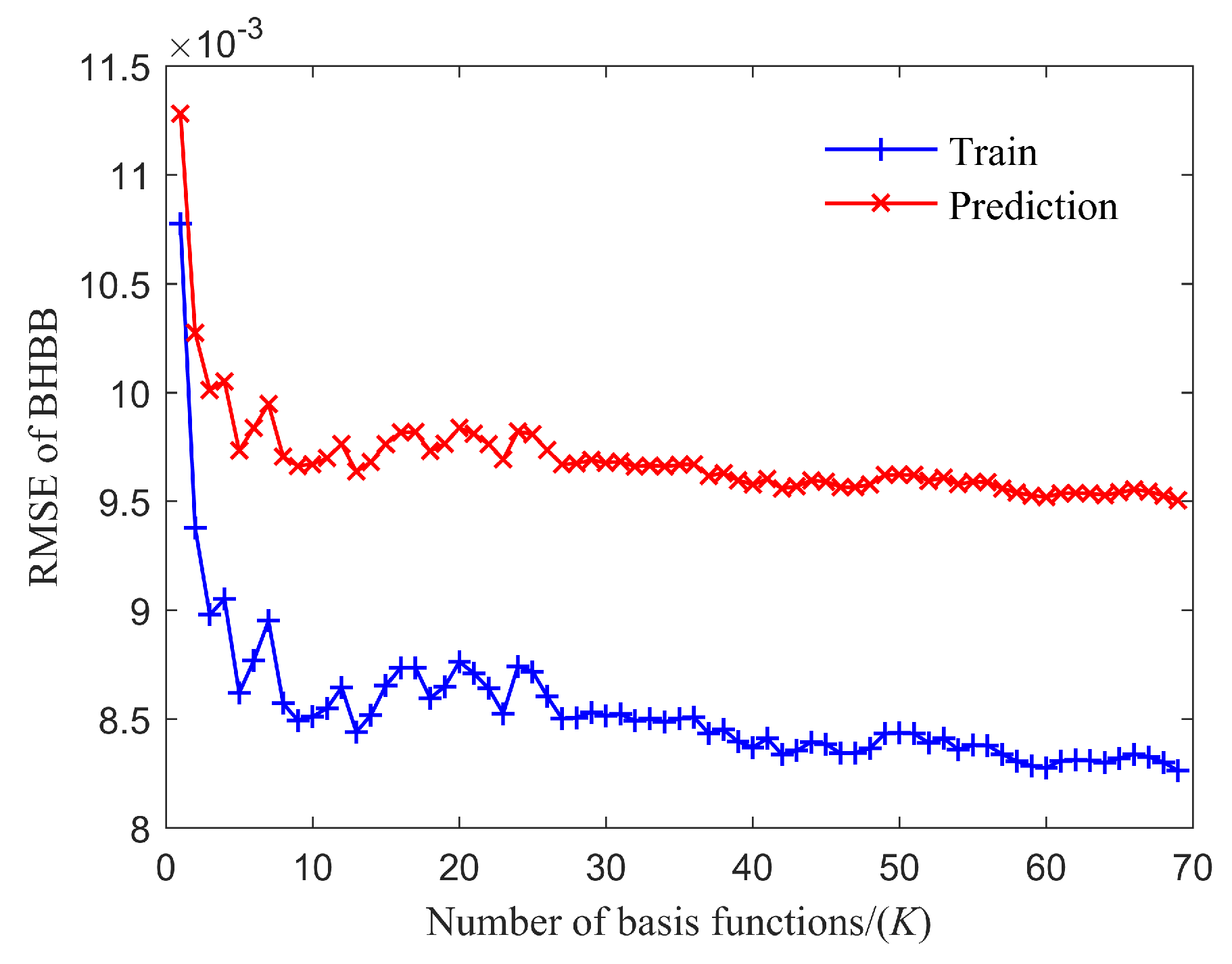
Based on the failure rate sample in Section 2, to select an appropriate parameter K, the relationship between the root mean-squared-error (RMSE) and the number of basis functions K is shown in Figure 3. It provides an example of RMSE based on the XZ. It depicts that the prediction RMSE has a huge improvement when K is less than 30. In addition, the RMSE value tends to stabilize after nearly 30 replications. It means that the results would be hard to improve with more bootstrap replicates. Hence, we set K = 30 in this paper. It takes about one and a half hours to complete the training of 30 sub-models in a single line for 5000 samplings.

4. Failure Evaluation of PME on BHBB

4.1. Prior Specification

After establishing the BHBB model, assigning of the prior distribution of model parameters is required. The prior distribution of model parameters is required to be assigned since it is related to the convergence of the model. Particularly, the convergence of MCMC needs to be considered when different prior distributions are specified. The selection methods of prior distribution include (1) expert prior, (2) weak information prior, and (3) the value range of the parameter [23,24]. The weak information prior, such as normal distribution, is generally recommended when an expert prior cannot be obtained. Therefore, most of the parameters can be determined by using the weak information prior if the ranges are not limited.
The value β 0 and β a , p of the Weibull regression model are not limited. To specify appropriate priors for the hierarchical model, normal distribution is selected for β 0 and β a , p as the prior probability density function
f β a , p μ a , p , σ a , p = 1 2 π σ a , p 2 × exp 1 2 σ a , p 2 x μ a , p 2
where μ a , p and σ a , p are the mean and standard deviation, respectively. λ is the regularization parameter of λ β a , p in log( β ) and it should be greater than θ . Thus, it can be specified as no information distribution
λ Uniform ( 0 , 3 )
In the case where mean μ a , p and standard deviation σ a , p parameters are independently sampled, the distributions of the parameters are different. However, they also have an intrinsic relationship as a result of sampling from the same prior distribution β a , p . It means that the inferences affect the prediction of failure rate in other areas. Generally, the hierarchical model is more powerful than a single-layer structure because they represent knowledge at different layers of abstraction. Therefore, in the second layer of BHBB, the parameters μ a , p and σ a , p are estimated by normal prior and half-Cauchy prior in Equation (9) respectively, which is helpful to simplicity and computational stability
M a , p Normal 0 , σ μ 2 σ a , p , α HalfCauch ( 10 )
where σ μ is the variance. A larger value can be set to σ μ in the beginning and then adjust with the convergence of the model. Parameter ρ in (7) is the normal distribution, the mean and standard deviation of ρ have the same distribution as parameter μ a , p in Equation (11).

4.2. Model Parameter Estimation and Prediction

To obtain the prediction results, all the observed data of PME are used to update the prior distributions and yield posterior probabilities using Bayes’ theorem [25]. As for the joint posterior probability, it has the same formula of every repetition in bagging, which can be written as
p β 0 , β a , p , α , λ , m i , θ c Y m = p β 0 , β α , p , α , λ , m i , θ c , Y m p Y m L Y m θ w , θ c , m i p β a , p μ a , p , σ a , p x p m i ϕ i p β 0 p ( α ) p θ c p ( λ )
where L Y m θ w , θ c , m i is the likelihood which has the same form as Equation (6), θ w consists of β 0 , β a , p , α and λ , p ( Y m ) is the marginal density function. The posterior distribution formulations can be obtained by integrating out the rest parameters based on the marginal posterior density. To estimate parameter m i , the marginal posterior distribution p m i Y m of m i is evaluated as
p m i Y m = p β 0 , β a , p , α , λ , m i , θ c Y m d θ w d θ c
The posterior distribution of BHBB parameters are calculated each repetition in bagging, K total times is used to resample from Y . The predicted mean value of failure rate can be expressed as
E m i Y = 1 k m = 1 k p m i Y m d m i m
Furthermore, the known information and posterior distribution of parameters are obtained to predict the failure rate effectively in another area. If some new data z x , t is observed, which contain the environmental features in the new area, the predicted failure rate can be inferred as
p z x , t Y = 1 k m = 1 k f z x , t θ p θ Y m d θ m
where p θ Y m denotes the joint posterior probability in Equation (12), θ represents parameters θ w , m i , and θ c . f z x , t θ is the expected value under the condition of known parameters θ .
As a necessary indicator of failure rate evaluation, it is necessary to consider the reliability of PME. Generally, this prediction can be adopted to take reserve measures or set strategies and provide a guarantee for system continuous operation.
The reliability of the system indicates the ability to complete the assignment at the given time. For the BHBB, the reliability function can be inferred as
R ( t Y ) = 1 K m = 1 K exp 0 t P w k = y a , t , i d θ m
where the range of parameters R ( t Y ) is [0, 1], the P w ( k = y a , t , i ) is the function of Weibull posterior probability density. Particularly, the corresponding posterior sample can be used to calculate the confidence intervals (CI) of reliability.
To verify the effectiveness of the outlier model and accuracy of the BHBB, model averaging is used to compare the relative accuracy between the BHBB and the common HB model. It should be noted that the HB does not have an outlier identification structure and bagging. Information criterion can then be computed to compare models under exactly the same observations [26].
We use the widely applicable information criterion (WAIC) to evaluate the models, which is a fully Bayesian criterion for estimating out-of-sample expectations [27]. The WAIC can be defined as the following form
W A I C = 2 ( j = 1 N log p * y a , t , i j = 1 N V log P y a , t , i θ )
where p * y a , t , i is the Bayes predictive distribution, V log P y a , t , i θ ) represents the variance of log-likelihood of y a , t , i . The first item in Equation (17) is Bayes training loss, and the second piece of WAIC is the effective number of parameters.

4.3. Proposed Failure Rate Prediction Framework

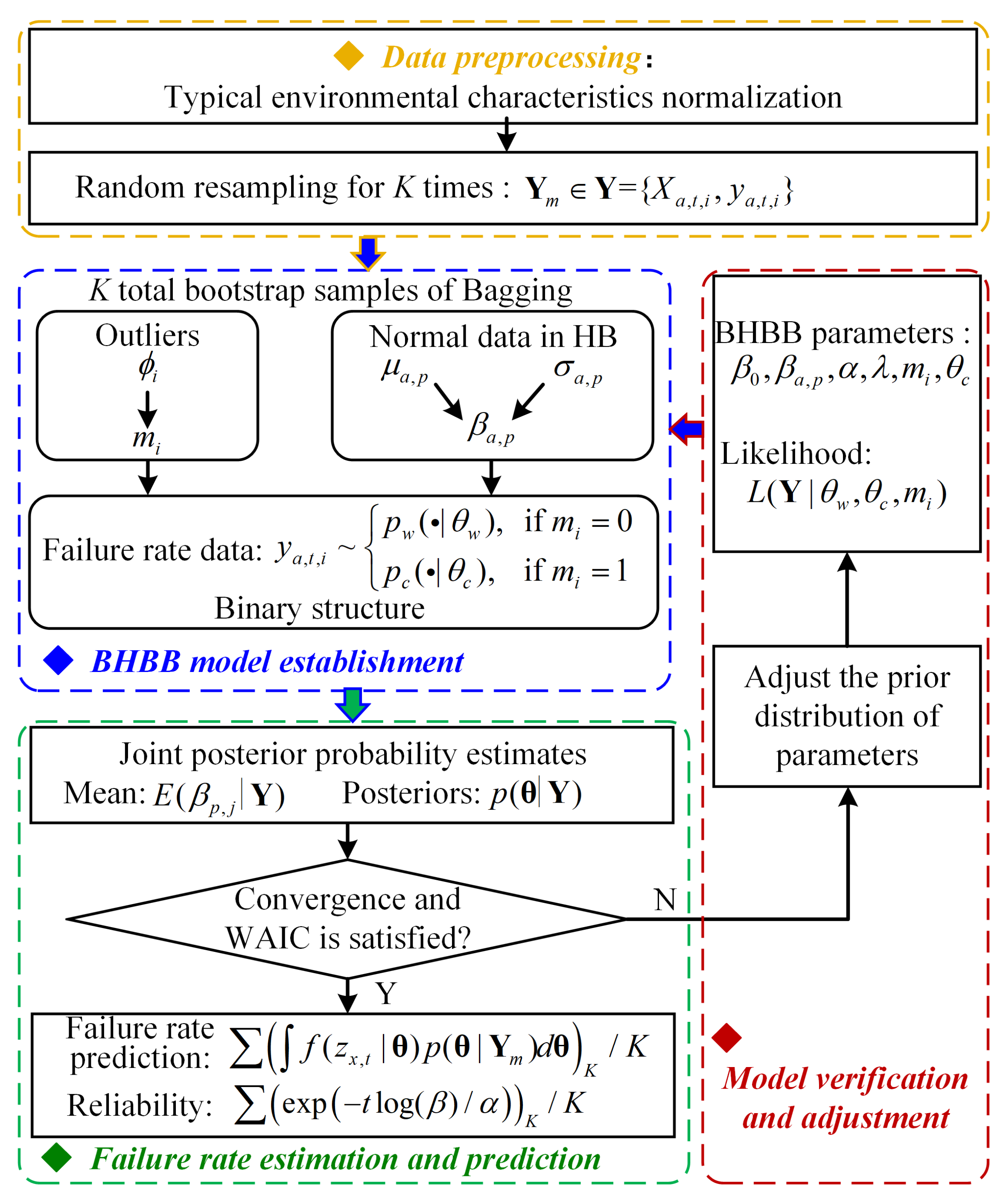
Aiming at solving the impact of environmental features and outlier in the failure rate data, a general BHBB framework is constructed and depicted in Figure 4. The framework can be divided into four steps.
1.
Data preprocessing: The environmental features and failure rates are normalized based on mean and standard deviation. The failure rate data is resampled for K times for the bagging algorithm and the Y m is obtained.
2.
Model establishment: The nonlinear regression model is built to integrate time and environmental features. For a particular experiment, every element in Y m is believed to have been generated by two models, i.e., a truly Weibull parameter model p w parameterized by θ w , and another outlier model pc parameterized by θ c . In this model, the binary parameter M = m i is defined as follows: m i = 0 if ith data point was generated by Weibull parameter model and m i = 1 if ith data point was generated by outlier model p c . Then the BHBB is established to predict the failure rate of PME based on bagging and outlier identification structure.
3.
Model estimation: The MCMC is used to generate samples from the posterior distribution. It takes a number of iterations for samples generated from the joint posterior distribution. Considering the convergence of the model, automatic differentiation variational inference is used to initialize all the parameter values. The results of the BHBB will average all K times posterior parameters.
4.
Model verification: The convergence analysis and WAIC are used to verify the validity of the model. If the convergence and WAIC do not meet the conditions, the model will use the trained model parameters to initialize or update priors to converge faster. Finally, the posterior distribution parameters are used to predict the failure rate and estimate the reliability.

5. Illustrative Example

To verify the effectiveness of the proposed BHBB, the Pymc3 is used, which is a kind of Python library. In the process of MCMC sampling, the number of samples is set to 5000 to fulfill all the samples and 2000 samples for burn-in. Considering the convergence of the model, automatic differentiation variational inference is used to initialize all the parameter values. Then No-U-Turn sampler and Binary-Gibbs-Metropolis are used to generate samples for continual distribution and discrete distribution, respectively [28]. To verify the effectiveness of the algorithm, leave-one-out cross-validation is used to separate data where 6 groups of data are used to training and 1 group for prediction per province.

5.1. Calculation: Model Comparison Analysis

In Equation (2), to select a suitable q value, the experiment with different parameter q is conducted to show its impact, as listed in Table 2. Here, the widely applicable information criterion (WAIC) and leave-one-out (LOO) cross-validation are used to evaluate the model, where a higher value means a better fitting effect.
As can be seen in Table 2, a higher q obtains better WAIC and LOO values. However, the training time is also increased when q equals 3. When q = 1 , it has the lowest WAIC and LOO values. Here, the q is set to 2 as a comprise between the model performance and training time.
To verify the fusion performance of the Bayesian model, the BHBB is compared with regular HB, multivariate regression methods PLSR [29], WN [29], GP [30], and SVM [31]. For a fair comparison, the number of layers and basic structure of HB is the same as BHBB. The size of sample data in each repetition of bagging is set to 15 in three areas, and the number of subset data m = 5 for each area in BHBB. In PLSR, the number of components to keep is set to 3 and the tolerance of the iterative algorithm is set 1 × 10⁻⁶. The nonlinear Wiener degradation structure in which the degradation parameters are integrated with environmental stress. The radial basis function (RBF) kernel is used in SVM. In addition, the penalty parameter and kernel coefficient are set to 1000 and 0.1, respectively. For GP, the RBF kernel is selected for the covariance functions. The performance of different models is evaluated through RMSE measures.
To verify the convergence of the BHBB, the z-scores proposed by Geweke are utilized to examine the MCMC chain. It compares the mean and variance at the beginning and end of the chain. The z-scores value should be located in [−2, 2], which indicates the MCMC is convergence. The z-scores results of four parameters from different layers of the BHBB are shown in Figure 5. It can be seen from Figure 5 that all the z-scores of different parameters are not exceeded ±0.5, indicating that the BHBB has great convergence.
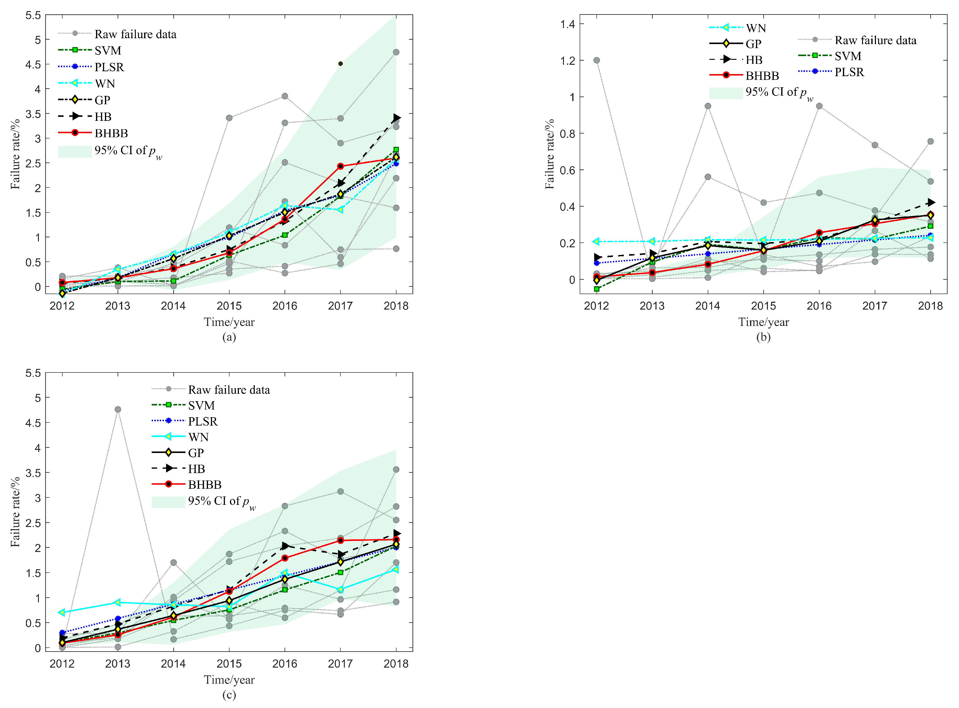
The predicted results in three areas are presented in Figure 6. It should be noted that the gray dots in each column represent the raw failure data points. For the PLSR, GP, and SVM, it shows that the results of PLSR, GP, and SVM can follow the trend of failure data, while the WN cannot. In addition, PLSR and WN cannot meet the characteristics of the failure rate data when considering environmental features. For example, the results of PLSR and WN in Figure 6b are straight lines, and they fail to capture the features of the failure rate. Additionally, the curve of SVM completely follows the data between 2013 and 2015 in Figure 6b, thus SVM is overfitting the failure data. Moreover, the prediction of SVM and GP is lower than zero in 2012 of Figure 6a,b. However, the failure rate should always be no less than zero.
For the regular HB, it can follow the change tendency of the failure rate data, indicating the effectiveness of the nonlinear regression. However, it shows that the curve of BHBB is smooth when integrating the features of the areas in Figure 6c. Both of the HB and BHBB can fit the data well in Figure 6a. However, it shows that the HB does not detect outliers because the curve is higher than the rest of the methods in Figure 6b.
As is clear from Figure 6b, some data points outside the 95% CI can be outliers in 2012, 2014, and 2016 of XJ. It shows that the mean curves generated by BHBB are more sensitive to outliers. However, the HB cannot identify outliers and change curve in Figure 6b,c. The 95% CI of p w shows the normal failure data, where the outside of CI are more likely to be outliers. The outliers outside the 95% CI can be assigned a smaller weight. In this example, the BHBB recognizes that not all the failure data coming from truly Weibull parameter model p w , the binary structure allows some outliers to fit the real world. Therefore, it is evident that the BHBB outperforms the other methods.
To highlight the effectiveness of the proposed method, the training and prediction RMSE of different methods are listed in Table 3. The RMSE is calculated from the mean of the curve. Additionally, the failure data outside the 95% CI are identified as outliers and, therefore, the outliers are replaced by the mean. It shows that the lowest predicted value of RMSE is BHBB, indicating that BHBB has a better precision performance. Furthermore, the comparison between BHBB and HB showed a significant improvement in prediction. Conversely, the RMSE of GP is lower than that of PLSR, WN, and HB. The highest RMSE is WN, which means that it has the worst fitting result. Intuitively, the results show that BHBB is more effective than traditional HB and deterministic approaches.
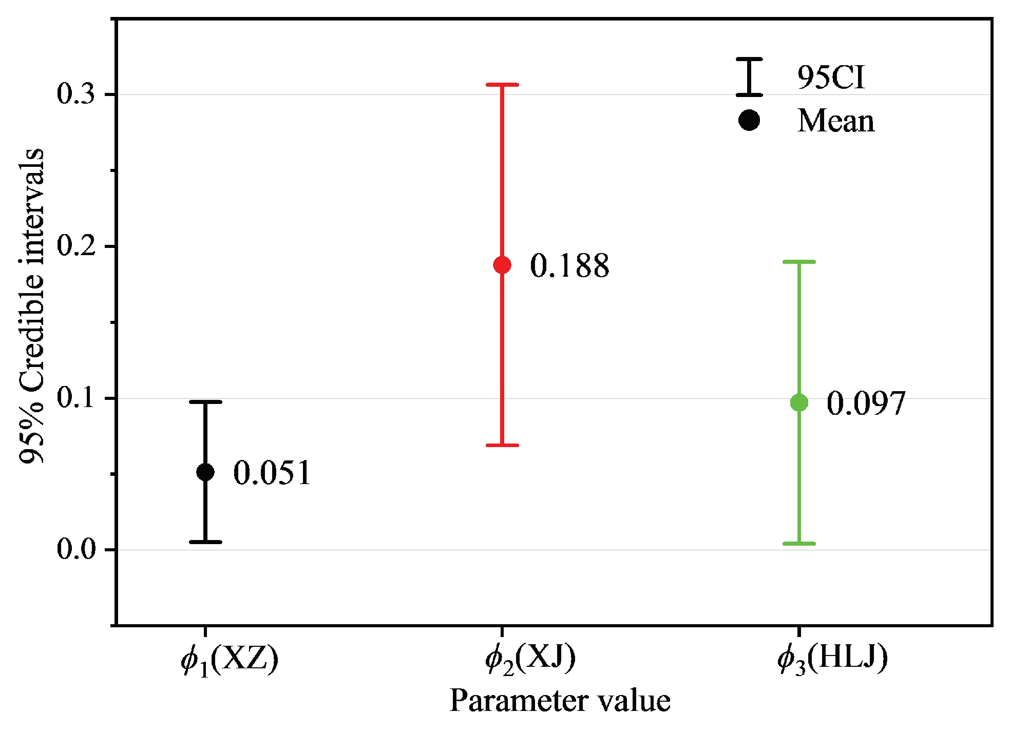
To verify the effectiveness of the outlier identification structure in BHBB, the mean and 95% CI of ϕ i in Equation (4) are depicted in Figure 7. ϕ i represents the proportion of outliers in the binary structure. It shows that the probability of outliers in XJ and HLJ is higher than XZ. The uncertain degree of outliers in XJ is larger due to more potential outliers leading to greater probability interval, which is consistent with the failure rate data according to Figure 6b. Broadly, the mean of the ϕ i in XZ is the smallest, indicating that the number of outliers is the least. Thus, it is worth mentioning that the BHBB has the ability to identify outliers from the failure rate data.
The value of WAIC is listed in Table 4. It worth mentioning that the pWAIC indicates the estimated effective number of parameters in models, which provides clues of how flexible each model is. A model r with larger weight w r means a better Bayesian model. The pWAIC of BHBB is greater than HB, it shows that BHBB is flexible than HB due to the outlier model. The difference between each WAIC and the lowest WAIC is depicted by dWAIC r . The huge dWAIC r of HB reveals the difference between the two models. The WAIC of BHBB is lower than HB and the value w r is higher than HB indicating the BHBB can make a better description for failure rate data.

5.2. Model Interpretation and Prediction of Reliability

Another advantage of BHBB is that the model parameters have physical meanings. Here, the mainly posterior quantities and CI of parameters are listed in Table 5.
The β 0 denotes the intercept of nonlinear regression in Equation (2). It is assumed that all the electrical meters samples have the same intercept due to producing by the same company. The β a , 1 is the slope of time, β a , 3 , and β a , 4 represent the slope of temperature and pressure, respectively. Different a ( a = 1 , 2 , 3 ) represents the slope of XZ, XJ, and HLJ in β a , p , respectively.
Table 5 shows that all the β a , 1 are positive and this indicates the failure rate has a strong correlation with time. More importantly, the first feature β a , 3 has a higher rate of contribution than the second feature β a , 4 , which means the higher temperature will cause more number of failures, and the electrical meters are sensitive to temperature changes while the pressure is constant.
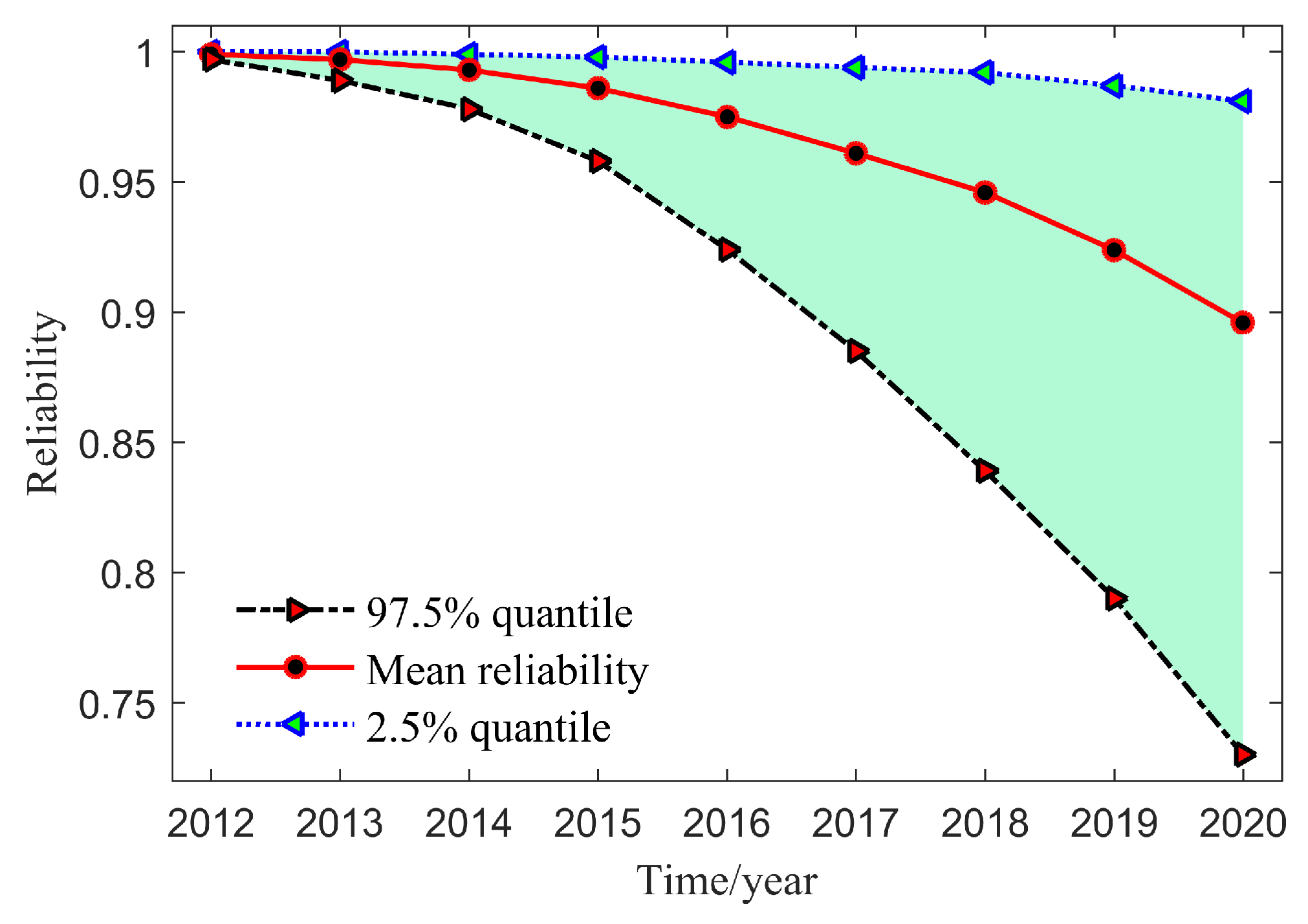
To predict the failure rate of electrical meters in the long term, the forecasting result of reliability is presented in Figure 8. This result is calculated using the reliability index in Equation (16). The quantile denotes the upper and lower bounds of the CI.
It is observed that the reliability of electrical meter declines over time. The value of reliability is nearly 0.965 in the sixth year. It also shows the electrical meters produced by its company have high reliability during the operation. On the other hand, the slope of the reliability curve is approximate a straight line and the uncertainty of this system is increasing, indicating the users do not need to change too much on the reserve and operate strategy in the short-term.
Overall, considering the security reliability of the PME in power system [32], a rotation strategy for practical PME reliability regulation and management can be developed so as to ensure the normal operation of PME. The PME can be replaced to prevent lack of equipment and reduce the cost of manufacturing, purchasing, and shipping.

6. Conclusions

In this paper, a binary hierarchical Bayesian with bagging method is proposed to evaluate the failure rate of PME from multiple typical locations. The inaccurate prediction results of failure rate and reliability in a small sample dataset with outliers have been addressed. This method overcomes the sole objective evaluation of failure rate, where multi-source information is embedded in BHBB. The visualization results of model parameters show that the model can identify outliers effectively for failure data of PME. Compared with the common hierarchical Bayesian and some traditional data-driven methods, the experiment manifests that the proposed method has superior performance in failure rate prediction even under a small sample dataset. The method adopts a combination of outlier identification structure and bagging, wherein the model parameters have the advantage of interpretability. Concretely, the convergence and variance experiments show that BHBB has great convergence and low RMSE. To further improve this methodology, future work will focus on the derivation of prior distribution in higher levels of hierarchical Bayesian.

Author Contributions

Conceptualization, J.L. and Q.T.; methodology, J.L. and W.Q.; software, J.M.; validation, J.L., W.Q. and J.M.; formal analysis, W.Q.; investigation, J.L.; data curation, J.D.; writing—original draft preparation, J.L.; writing—review and editing, Q.T. and W.Q.; visualization, J.M.; supervision, Q.T.; project administration, Q.T.; funding acquisition, Q.T. All authors have read and agreed to the published version of the manuscript.

Funding

This research was funded in part by National Key R & D Program of China OF FUNDER grant number 2019YFF0216800, and in part by Postgraduate Scientific Research Innovation Project of Hunan Province OF FUNDER grant number CX20200426.

Institutional Review Board Statement

Not applicable.

Informed Consent Statement

Not applicable.

Data Availability Statement

Not applicable.

Conflicts of Interest

The authors declare no conflict of interest.

References

  1. Conti, M.; Orcioni, S. Modeling of Failure Probability for Reliability and Component Reuse of Electric and Electronic Equipment. Energies 2020, 13, 2843. [Google Scholar] [CrossRef]
  2. Wang, H.; Liu, Z.; Xu, Y.; Wei, X.; Wang, L. Short text mining framework with specific design for operation and maintenance of power equipment. CSEE J. Power Energy Syst. 2020, 1, 1–10. [Google Scholar]
  3. Devlin, M.A.; Hayes, B.P. Non-Intrusive Load Monitoring and Classification of Activities of Daily Living Using Residential Smart Meter Data. IEEE Trans. Consum. Electron. 2019, 65, 339–348. [Google Scholar] [CrossRef]
  4. Alahakoon, D.; Yu, X. Smart Electricity Meter Data Intelligence for Future Energy Systems: A Survey. IEEE Trans. Ind. Inform. 2016, 12, 425–436. [Google Scholar] [CrossRef]
  5. Sun, K.; Xiao, H.; Pan, J.; Liu, Y. A Station-Hybrid HVDC System Structure and Control Strategies for Cross-Seam Power Transmission. IEEE Trans. Power Syst. 2021, 36, 379–388. [Google Scholar] [CrossRef]
  6. Liu, H.; Wang, Y.; Yang, Y.; Liao, R.; Geng, Y.; Zhou, L. A Failure Probability Calculation Method for Power Equipment Based on Multi-Characteristic Parameters. Energies 2017, 10, 704. [Google Scholar] [CrossRef] [Green Version]
  7. Qiu, W.; Tang, Q.; Teng, Z.; Yao, W.; Qiu, J. Failure rate prediction of electrical meters based on weighted hierarchical Bayesian. Measurement 2019, 142, 21–29. [Google Scholar] [CrossRef]
  8. Jin, L.; Peng, C.; Jiang, T. System-Level Electric Field Exposure Assessment by the Fault Tree Analysis. IEEE Trans. Electromagn. Compat. 2017, 59, 1095–1102. [Google Scholar] [CrossRef]
  9. Zhu, P.; Han, J.; Liu, L.; Lombardi, F. A Stochastic Approach for the Analysis of Dynamic Fault Trees With Spare Gates Under Probabilistic Common Cause Failures. IEEE Trans. Reliab. 2015, 64, 878–892. [Google Scholar] [CrossRef]
  10. Lu, J.; Huang, J.; Lu, F. Sensor Fault Diagnosis for Aero Engine Based on Online Sequential Extreme Learning Machine with Memory Principle. Energies 2017, 10, 39. [Google Scholar] [CrossRef] [Green Version]
  11. Lu, F.; Jiang, C.; Huang, J.; Wang, Y.; You, C. A Novel Data Hierarchical Fusion Method for Gas Turbine Engine Performance Fault Diagnosis. Energies 2016, 9, 828. [Google Scholar] [CrossRef] [Green Version]
  12. Yang, Z.; Chen, Y.; Li, Y.; Zio, E.; Kang, R. Smart electricity meter reliability prediction based on accelerated degradation testing and modeling. Int. J. Electr. Power Energy Syst. 2014, 56, 209–219. [Google Scholar] [CrossRef] [Green Version]
  13. Xu, D.; Wei, Q.; Elsayed, E.A.; Chen, Y.; Kang, R. Multivariate Degradation Modeling of Smart Electricity Meter with Multiple Performance Characteristics via Vine Copulas. Qual. Reliab. Eng. Int. 2017, 33, 803–821. [Google Scholar] [CrossRef]
  14. Sundaravadivel, P.; Kesavan, K.; Kesavan, L.; Mohanty, S.P.; Kougianos, E. Smart-Log: A Deep-Learning Based Automated Nutrition Monitoring System in the IoT. IEEE Trans. Consum. Electron. 2018, 64, 390–398. [Google Scholar] [CrossRef]
  15. Yuan, T.; Kuo, Y. Bayesian Analysis of Hazard Rate, Change Point, and Cost-Optimal Burn-In Time for Electronic Devices. IEEE Trans. Reliab. 2010, 59, 132–138. [Google Scholar] [CrossRef]
  16. Mishra, M.; Martinsson, J.; Rantatalo, M.; Goebel, K. Bayesian hierarchical model-based prognostics for lithium-ion batteries. Reliab. Eng. Syst. Saf. 2018, 172, 25–35. [Google Scholar] [CrossRef]
  17. Zhang, Y.; Li, M.; Dong, Z.Y.; Meng, K. Probabilistic anomaly detection approach for data-driven wind turbine condition monitoring. CSEE J. Power Energy Syst. 2019, 5, 149–158. [Google Scholar] [CrossRef]
  18. Brown, R.E.; Frimpong, G.; Willis, H.L. Failure rate modeling using equipment inspection data. IEEE Trans. Power Syst. 2004, 19, 782–787. [Google Scholar] [CrossRef]
  19. State Grid Corporation of China, Technical specification for single phase smart electricity meters, Q/GDW 1364-2013. 2013. Available online: https://ishare.iask.sina.com.cn/ (accessed on 10 May 2021).
  20. National Meteorological Information Center. 2021. Available online: http://data.cma.cn/ (accessed on 20 May 2021).
  21. Ciani, L.; Guidi, G. Application and analysis of methods for the evaluation of failure rate distribution parameters for avionics components. Measurement 2019, 139, 258–269. [Google Scholar] [CrossRef]
  22. Salehi, M.; Leckie, C.; Bezdek, J.C.; Vaithianathan, T.; Zhang, X. Fast Memory Efficient Local Outlier Detection in Data Streams. IEEE Trans. Knowl. Data Eng. 2016, 28, 3246–3260. [Google Scholar] [CrossRef]
  23. Gevaert, O.; De Smet, F.; Kirk, E.; Van Calster, B. Predicting the outcome of pregnancies of unknown location: Bayesian networks with expert prior information compared to logistic regression. Hum. Reprod. 2006, 21, 1824–1831. [Google Scholar] [CrossRef] [Green Version]
  24. Qiu, W.; Tang, Q.; Yao, W.; Qin, Y.; Ma, J. Probability Analysis for Failure Assessment of Electric Energy Metering Equipment Under Multiple Extreme Stresses. IEEE Trans. Ind. Inform. 2021, 17, 3762–3771. [Google Scholar] [CrossRef]
  25. Gadrich, T.; Bashkansky, E. A Bayesian approach to evaluating uncertainty of inaccurate categorical measurements. Measurement 2016, 91, 186–193. [Google Scholar] [CrossRef]
  26. Kontar, R.; Zhou, S.; Sankavaram, C.; Du, X.; Zhang, Y. Nonparametric-Condition-Based Remaining Useful Life Prediction Incorporating External Factors. IEEE Trans. Reliab. 2018, 67, 41–52. [Google Scholar] [CrossRef]
  27. Watanabe, S.; Opper, M. Asymptotic Equivalence of Bayes Cross Validation and Widely Applicable Information Criterion in Singular Learning Theory. J. Mach. Learn. Res. 2010, 11, 3571–3594. [Google Scholar]
  28. Alexander, M.; Zagheni, E.; Barbieri, M. A Flexible Bayesian Model for Estimating Subnational Mortality. Demography 2017, 54, 2025–2041. [Google Scholar] [CrossRef] [PubMed]
  29. Hosani, E.A.; Meribout, M.; Al-Durra, A.; Al-Wahedi, K.; Teniou, S. A New Optical-Based Device for Online Black Powder Detection in Gas Pipelines. IEEE Trans. Instrum. Meas. 2014, 63, 2238–2252. [Google Scholar] [CrossRef]
  30. Rasmussen, C.E. Distributed Computing and Internet Technology. In Summer School on Machine Learning; Springer: Berlin/Heidelberg, Germany, 2004; pp. 63–71. [Google Scholar]
  31. Wang, S.; Ding, X.; Zhu, D.; Yu, H.; Wang, H. Measurement uncertainty evaluation in whiplash test model via neural network and support vector machine-based Monte Carlo method. Measurement 2018, 119, 229–245. [Google Scholar] [CrossRef]
  32. Bashian, A.; Assili, M.; Anvari-Moghaddam, A. A security-based observability method for optimal PMU-sensor placement in WAMS. Int. J. Electr. Power Energy Syst. 2020, 121, 106157. [Google Scholar] [CrossRef]
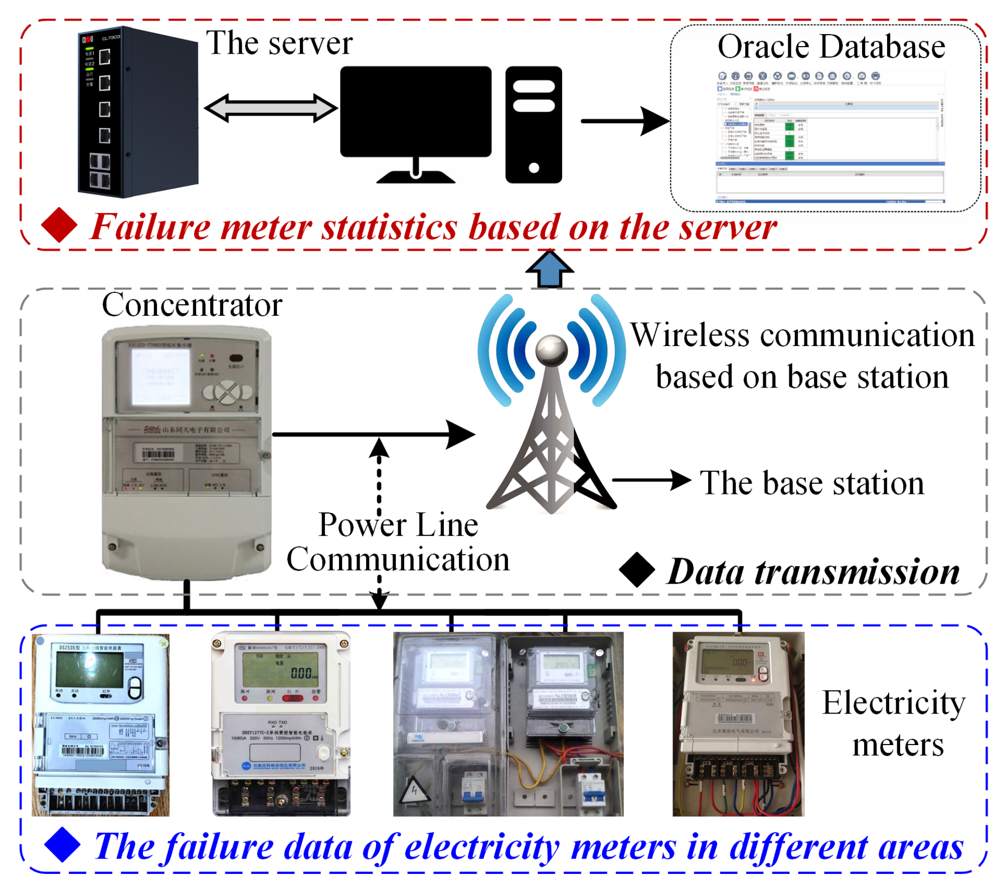
Figure 1. Operation status monitoring platform of the electrical meters.
Energies 14 03632 g001
Figure 2. The raw failure rate data of electrical meters from (a) XZ, (b) XJ, and (c) HLJ.
Energies 14 03632 g002
Figure 3. RMSE curve of BHBB for training and prediction in XZ.
Energies 14 03632 g003
Figure 4. The BHBB framework for failure evaluation of PME.
Energies 14 03632 g004
Figure 5. The BHBB framework for failure evaluation of PME.
Energies 14 03632 g005
Figure 6. Failure rate prediction results of the four methods including SVM, PLSR, WN, GP, HB, and BHBB in (a) XZ, (b) XJ, and (c) HLJ.
Energies 14 03632 g006
Figure 7. The confidence interval of ϕ i for outlier identification structure in BHBB.
Energies 14 03632 g007
Figure 8. The prediction curve for the reliability of electrical meters. The quantile represents the boundary value of the CI.
Energies 14 03632 g008
Table 1. Environmental features of true typical areas.
AreasM-Tem (℃)N-Tem (℃)Pre. (hPa)Hum. (%RH)Ill. (Lux)
XZ29−10605.261.9103.8
XJ47−221003.528.3327.64
HLJ37−31925.255.7253.6
Table 2. Performance comparison of different q value.
q ValueWAICLOOTraining Time
1101.2104.7470.5 s
2130.5128.8366.7 s
3165146.1799.0 s
Table 3. Comparison of training and prediction RMSE results.
ModelXZXJHLJ
TrainingPLSR 0.861 × 10 2 0.258 × 10 2 0.797 × 10 2
SVM 0.857 × 10 2 0.269 × 10 2 0.869 × 10 2
WN 0.924 × 10 2 0.317 × 10 2 0.919 × 10 2
GP 0.862 × 10 2 0.265 × 10 2 0.817 × 10 2
HB 0.903 × 10 2 0.259 × 10 2 0.821 × 10 2
BHBB 0.855 × 10 2 0.261 × 10 2 0.811 × 10 2
PredictionPLSR 0.124 × 10 1 0.307 × 10 2 0.110 × 10 1
SVM 0.109 × 10 1 0.296 × 10 2 0.866 × 10 2
WN 0.143 × 10 1 0.335 × 10 2 0.132 × 10 1
GP 0.103 × 10 1 0.275 × 10 2 0.832 × 10 2
HB 0.127 × 10 1 0.304 × 10 2 0.115 × 10 1
BHBB 0.965 × 10 2 0.271 × 10 2 0.812 × 10 2
Table 4. WAIC value of BHBB and HB under model averaging.
ModelWAICpWAICdWAICr w r
BHBB17.1120.8401
HB114.1417.9397.030
Table 5. Main parameter values of BHBB.
ParameterMeanSDConfidence Interval
β a , p 2.50%97.50%
β 0 −0.7841.877−4.6212.824
β 0 , 1 0.6280.0680.4960.772
β 1 , 1 0.580.0880.4240.771
β 2 , 1 0.5240.0780.3620.663
β 0 , 3 0.3690.462−0.541.21
β 1 , 3 0.3120.441−0.5211.22
β 2 , 3 0.1440.326−0.4090.884
β 0 , 4 −0.3851.916−3.8793.32
β 1 , 4 0.8451.944−3.1625.207
β 2 , 4 2.4924.181−4.10811.52
Publisher’s Note: MDPI stays neutral with regard to jurisdictional claims in published maps and institutional affiliations.