Abstract
Three-phase wye–delta LLC topology is suitable for voltage step down and high output current, and has been used in the industry for some time, e.g., for server power and EV charger. However, no comprehensive circuit analysis has been performed for three-phase wye–delta LLC. This paper provides complete analysis methods for three-phase wye–delta LLC. The analysis methods include circuit operation, time domain analysis, frequency domain analysis, and state–plane analysis. Circuit operation helps determine the circuit composition and operation sequence. Time domain analysis helps understand the detail operation, equivalent circuit model, and circuit equation. Frequency domain analysis helps obtain the curve of the transfer function and assists in circuit design. State–plane analysis is used for optimal trajectory control (OTC). These analyses not only can calculate the voltage/current stress, but can also help design three-phase wye-delta connected LLC and provide the OTC control reference. In addition, this paper uses PSIM simulation to verify the correctness of analysis. At the end, a 5-kW three-phase wye–delta LLC prototype is realized. The specification of the prototype is a DC input voltage of 380 V and output voltage/current of 48 V/105 A. The peak efficiency is 96.57%.
1. Introduction
With the popularity and rapid progress of electronic products, power electronic technology is also constantly improving. Most power converters have been developing in the direction of high efficiency, high power, and high power density due to the demand for consumer electronics. The LLC resonant converter meets the above requirements and is one of the commonly used topologies in recent years, e.g., for server powers, EV chargers, LED drivers, renewable power systems, and wireless power transfer systems [1,2,3,4,5]. There are many advantages, such as zero-voltage switching (ZVS) on the primary side and zero-current switching (ZCS) [6,7] on the secondary side, that can effectively improve the efficiency and increase the feasibility of high switching frequency. Moreover, the disadvantages of LLC are high ripple current in the output capacitor and narrow output voltage range [8]. However, the development and application has become quicker and wider, e.g., with the battery charger. From consumer electronics, server power, to electric vehicle, battery charge technology is everywhere [9,10]. The application voltage ranges from tens of volts to hundreds of volts, even up to kilo volts. The power of the battery charger converter is increasing too. In this kind of situation, the traditional LLC is not entirely suitable for the requirements. To solve the problem, if the converter is paralyzed to promote the power level, it will have more issues, such as current sharing problem [11,12] or system stability reduction. Several papers provide a three-phase wye-connected LLC topology to reduce the current sharing problem. Wye-connected LLC topology can not only reduce the current sharing problem, but also substantially reduce the output current ripple [13]. Low output current ripple is a good characteristic because high output current ripple will increase the output voltage ripple and reduce the output capacitor lifetime. However, three-phase LLC presents high ripple current in output capacitor and narrow output voltage range, together with improved power level, high efficiency, and good output characteristics [14]. Therefore, the application of wye-connected or delta-connected topology on the primary and secondary sides is gradually being studied.
According to the combination of wye-connected and delta-connected topology in the primary and secondary sides, the connection type can be divided into wye–wye, wye–delta, delta–wye, and delta–delta [15,16,17]. In wye-connected topology, the voltage stress of component is times that of traditional voltage stress. In delta-connected topology, the current stress of component is times that of traditional current stress. Thus, the wye-connected topology is suitable for higher voltage situations, and delta-connected topology is suitable for higher current situations.
This paper aims to analyze the three-phase wye–delta LLC topology by providing a complete analysis for reference in practical design situations. First, the circuit composition and operation are introduced. Second, time domain analysis is used to list the state equations of the resonant tank. Time domain analysis is a more accurate circuit analysis, but the calculation is complicated [18]. The time domain analysis can help the designer to run circuit simulation and optimal trajectory control (OTC) [19]. Then, frequency domain analysis uses the first hormonic aproximation (FHA) method to simplify the analysis and obtain the output voltage gain curve [20]. The frequency domain analysis can help the designer to design the control loop in LLC. However, in order to improve the accuracy of the gain curve to optimize the circuit, additional calculations for the circuit specifications and applications remain necessary [21,22]. Finally, the time domain equation is used to derive the state–plane graph. The state–plane graph not only can find the voltage/current stress on resonant components but also helps design the optimal trajectory control [23,24]. OTC is a new control method recently developed. It can effectively improve the transient and startup characteristics of LLC circuits.
After introducing the analysis of three-phase wye–delta LLC topology, this paper finally realizes a 5-kW prototype with DC input voltage of 380 V, output voltage of 48 V, and output current of 105 A. The highest efficiency is 96.57%.
2. Three-Phase Wye-Delta LLC
2.1. Topology
Figure 1 shows that three-phase wye–delta LLC is composed of three sets of half-bridge LLC. Each half-bridge is connected to a resonant tank and a transformer separately. Three transformers are connected to one another in wye type in the primary side, and the secondary side is connected in delta type. Ideally, the characteristic values of three resonance tanks need to be as close as possible, and the relationship of line voltage and phase voltage is .
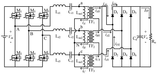
Figure 1.
Topology of three-phase wye–delta LLC.
2.2. Operation Principle
The control method of three-phase wye–delta LLC is pulse frequency modulation. Each set of half-bridge signal is in 120-degree phase-shift, and each duty cycle is almost 50%. The different operation sequence leads secondary current phase-lead or phase-lag. Figure 2 shows that, if the signal lags 120 degrees in sequence, then current will lag θ degree after switch A. For another case, if the signal leads than A 120 degrees in sequence, then current will lead θ degree before switch A.
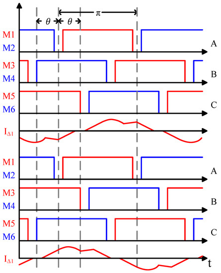
Figure 2.
Influence of switching at deferent sequence.
2.3. Time Domain Analysis
To simplify the analysis, this paper defines three hypotheses:
- The body diode of MOSFET is considered, and parasitic capacity is neglected.
- Output capacity is immense, and output can be seen as an ideal voltage source.
- All components are ideal.
Based on the hypothesis, the operation station delivers 12 parts. The operation of the positive half cycle is the same as that of the negative half cycle. Hence, the time domain analysis only describes at the positive half cycle. Furthermore, the operation of three sets of A, B, and C are in 120-degree phase-shift, and subsequently only focus on set A. Figure 3 presents the operation station of three-phase wye–delta LLC.
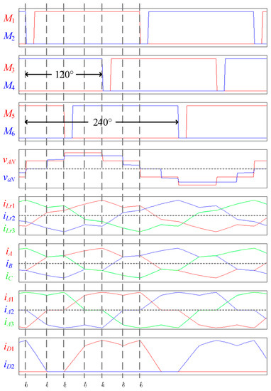
Figure 3.
Operation station of three-phase wye–delta LLC.
- 1.
- Stage 1: t0 < t < t1
In Figure 4a, switch is turned off, switches and keep turned on, switches and keep turned off, and switch is turned on after a short dead time. Current passes though body diode of switch . The voltage of steps up from to . Secondary diode starts to conduct. Hence, TF1 is forced short circuit and decoupled. After dead time, switch is turned on, and soft switch is completed. Current falls, current rises until equal to , then Stage 1 is finished. Figure 4b is the equivalent circuit, and the state equation of the resonant tank follows.
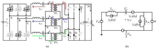
Figure 4.
(a) Circuit station at Stage 1 (b) Equivalent circuit at Stage 1.
- 2.
- Stage 2: t1 < t < t2
In Figure 5a, all switches’ states are the same as Stage 1. Current and are in series; hence, current is zero. The primary side of TF1 and TF3 are seen as parallel, and the secondary side of TF1 and TF3 are seen as series. Transformer voltage , noted here as , is determined by the state of the resonant tank. All transformers transfer energy to the secondary side at the same time. Figure 5b shows the equivalent circuit, and the state equation of the resonant tank follows.
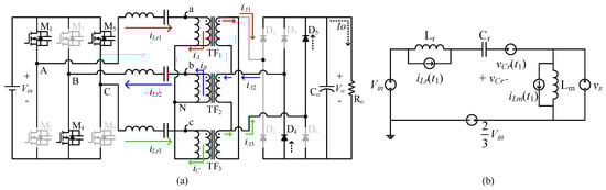
Figure 5.
(a) Circuit station at Stage 2 (b) Equivalent circuit at Stage 2.
- 3.
- Stage 3: t2 < t < t3
In Figure 6a, switch is turned off, switches and keep turned on, switches and keep turned off, and switch is turned on after a short dead time. Current passes though body diode of switch . The voltage of steps up from to . Secondary diode starts to conduct. Hence, TF3 is forced short circuit and decoupled. After dead time, switch is turned on, and soft switch is completed. Current falls, current rises until equal to , then Stage 3 is finished. Figure 6b is the equivalent circuit, and the state equation of the resonant tank follows.
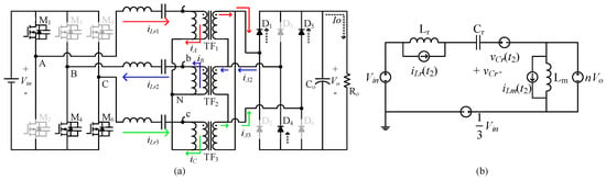
Figure 6.
(a) Circuit station at Stage 3 (b) Equivalent circuit at Stage 3.
- 4.
- Stage 4: t3 < t < t4
In Figure 7a, all switches’ states are the same as Stage 3. Current and are in series. Hence, current is zero. The primary side of TF2 and TF3 are seen as parallel, and the secondary side of TF2 and TF3 are seen as series. Transformer voltage is determined by the state of the resonant tank. All transformers transfer energy to the secondary side at the same time. Figure 7b is the equivalent circuit, and the state equation of the resonant tank follows.
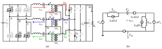
Figure 7.
(a) Circuit station at Stage 4 (b) Equivalent circuit at Stage 4.
- 5.
- Stage 5: t4 < t < t5
In Figure 8a, switch is turned off, switches and keep turned on, switches and keep turned off, and switch is turned on after a short dead time. Current passes though body diode of switch . The voltage of steps up from to . Secondary diode starts to conduct. Hence, TF2 is forced to short circuit and decoupled. After dead time, switch is turned on, and soft switch is completed. Current falls, current rises until equal to , then Stage 5 is finished. Figure 8b is the equivalent circuit, and the state equation of the resonant tank follows.
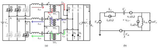
Figure 8.
(a) Circuit station at Stage 5 (b) Equivalent circuit at Stage 5.
- 6.
- Stage 6: t5 < t < t6
In Figure 9a, all switch states are the same as Stage 5. Current and are in series. Hence, current is zero. The primary side of TF1 and TF2 are seen as parallel, and the secondary side of TF1 and TF2 are seen as series. Transformer voltage , noted here as , is determined by the state of the resonant tank. All transformers transfer energy to the secondary side at the same time. Figure 9b is the equivalent circuit, and the state equation of the resonant tank follows.
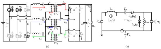
Figure 9.
(a) Circuit station at Stage 6 (b) Equivalent circuit at Stage 6.
2.4. Frequency Domain Analysis
The operation waveform should be simplified to use FHA to derive the transfer function. Figure 10 shows the operation waveform of the resonant tank and transformer.
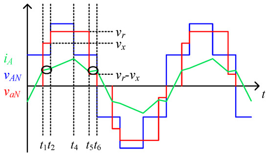
Figure 10.
Operation waveform of resonant tank and transformer.
In Figure 10, the value of current is similar at and , and the lengths of time are the same. To facilitate FHA calculations, can be seen as a sine wave and can be seen as a square wave, as shown in Figure 11.
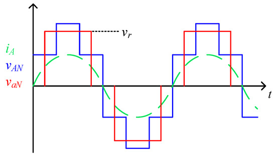
Figure 11.
Simplified waveform of resonant tank and transformer.
The FHA coefficients of , , and can be calculated, as shown in Table 1. Furthermore, the topology gain can be divided into five parts per cycle. The equation is as follows:

Table 1.
Function and FHA coefficient.
Based on the above result, transfer gain can be calculated as follows:
where is the transfer function of . The value is same as LLC. Thus, the gain curve of three-phase wye–delta LLC is similar to that of conventional LLC. The only difference is that the gain has a coefficient.
2.5. State-Plane Analysis
Application for state–plane analysis: This analysis can determine the resonant voltage/current stress and operating state. It can also assist in the design of OTC. OTC can effectively improve the transient and reduce the voltage/current stress of startup of LLC circuits. This section uses the circuit equation to calculate the voltage/current state of the resonance tank accurately, then uses standardization and geometric principle to depict the resonant voltage and current state. First, six initial values of the equation need to be obtained. The definitions and descriptions are shown in Figure 12 and Table 2.
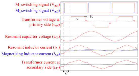
Figure 12.
Waveform of six variables.
Table 2.
Describe of six variables.
To determine the six initial values, six equations must be listed, as shown below:
- 1.
- Symmetry of magnetizing inductor current
In Figure 13, assuming that , it can be listed.
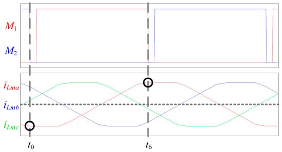
Figure 13.
Waveform of symmetrical magnetizing inductor current.
The attached Equation (A15) (Appendix A) is used to substitute Equation (21) and obtain:
- 2.
- Symmetry of resonant inductor current
In Figure 14, because of the symmetry of resonant inductor current, it can be listed.
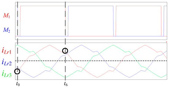
Figure 14.
Waveform of symmetrical resonant inductor current.
The attached Equation (A13) is used to substitute Equation (23) and obtain:
- 3.
- Symmetry of resonant capacitor voltage
In Figure 15, because of the symmetry of resonant inductor current, it can be listed.
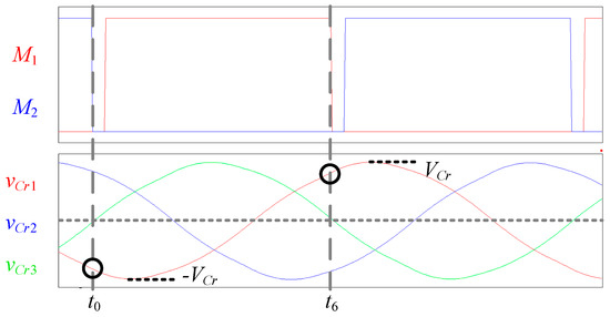
Figure 15.
Waveform of symmetrical resonant capacitor voltage.
The attached Equation (A14) is used to substitute Equation (25) and obtain:
- 4.
- Conservation of energy
Since each phase provides of input power, the average absolute value of the primary side resonance current is also of the input current. Furthermore, the capacitor voltage is changed from to . Therefore, the equation for the voltage change of the resonant capacitor in a half cycle can be:
is used to substitute Equation (28) and obtain:
- 5.
- The current is equal at the secondary side when .
In Figure 16, when , and current is equal to , then it can be listed.
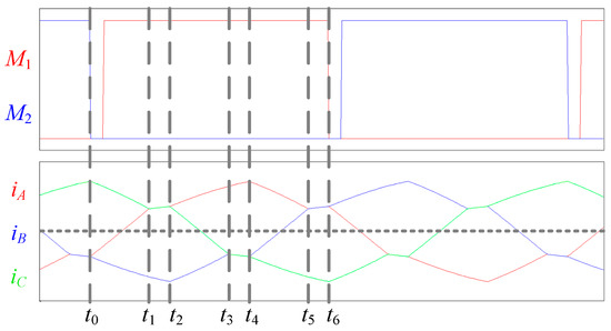
Figure 16.
Waveform of transformer current.
In addition, the resonant current includes the magnetizing current and the current coupled from the secondary side. Thus, the formula can be rewritten as:
The attached Equations (A4), (A6), (A13), and (A15) are used to substitute Equation (31) and obtain:
- 6.
- The current is equal at the secondary side when
Similar to the above, when , and current is equal to , then it can be listed.
The attached Equations (A4), (A6), (A13), and (A15) are used to substitute Equation (33) and obtain:
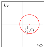
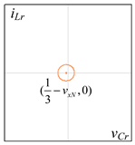
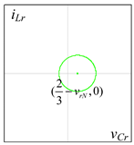
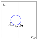
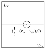
The six initial values can be solved using the above six Equations (22), (24), (26), (29), (32), and (34) and determine the output load. Normalization is necessary to depict the state plane. By normalizing and with voltage factor and current factor , the state–plane can be depicted, as shown in Figure 17a. In addition, the value and value also shown in Figure 17b. Among them, the is characteristic impedance, where . All normalized state equations and individual trajectories are shown in Table 3.
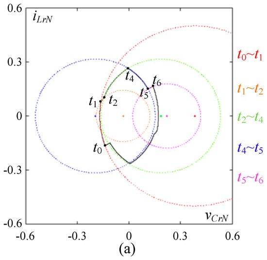
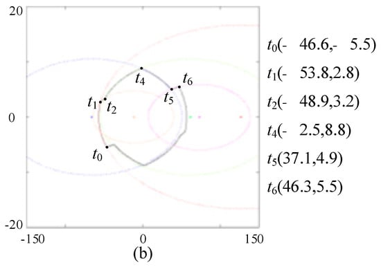
Figure 17.
State–plane schematic diagram at 50% load. (a) normalizing form(b) real value form.
Table 3.
Equations and state–plane trajectory.
3. Design and Simulation Verification
This paper designs a prototype and performs PSIM simulation to verify the accuracy of the analysis. Table 4 and Table 5 show the specifications of the circuit design and the parameters of the resonant tank, respectively. The output power is about 5 kW, and three sets of resonant parameter values are equal.
Table 4.
Specification of three-phase wye–delta LLC.
Table 5.
Parameters of resonant tank.
Figure 18, Figure 19 and Figure 20 show the gain curve comparison of analysis and the PSIM simulation. The load conditions of 2.4, 0.96, and 0.457 ohm are in sequence. The figures show that the trend of the gain curve is much closed. The maximum difference of switching frequency at the voltage regulation point is about 25 kHz.
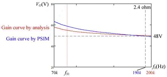
Figure 18.
Gain curve comparison at 20% load.
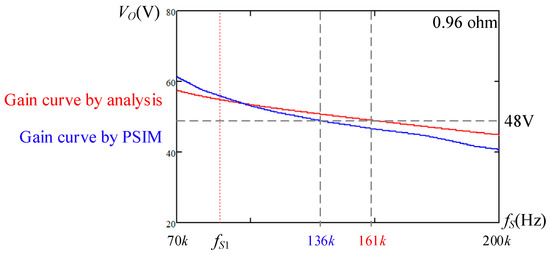
Figure 19.
Gain curve comparison at 50% load.
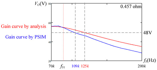
Figure 20.
Gain curve comparison at 100% load.
4. Experimental Results
This paper uses Table 4 as the specification to realize a prototype 5-kW three-phase wye–delta LLC. Figure 21 shows the operational waveform at 50% and 100% loads. In Figure 21, the peak currents of 50% and 100% loads are 8.85 A and 17.47 A, respectively. Figure 22 shows the state–plane from the PSIM simulation. Compared with Figure 17b, the value is closed, the max error of current is 0.2 A, and the max error of voltage is 1.7 V.
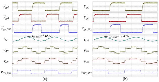
Figure 21.
(a) Experiment waveform at 50% load (b) Experiment waveform at 100% load. (Time: 2 µs/div; Vgs1: 2 V/div; Vgs2: 2 V/div; Vgs_SR2: 2 V/div). ((a) iLr1: 5 A/div; (b) iLr1: 10 A/div; vAN: 100 V/div; vaN: 100 V/div; vDS_SR2: 20 V/div).
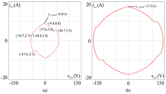
Figure 22.
(a) State-plane analysis result at 50% load (b) State-plane analysis result at 100% load.
Figure 23 shows the current statement of three resonant inductors at 50% load. The three resonant currents have no unbalanced current problem. In addition, a higher frequency ripple shows at . The reason for this is that the secondary winding of transformer is copper sheet, and it does not use the sandwich winding method. Thus, the coupling capacity is evident. It causes the resonant inductor to oscillate with the parasitic capacitor of transformer. Figure 24 shows the efficiency from light load to 100% load. The highest efficiency point is 96.57%, and the full load efficiency is 93.74%. All equipment including power source, load, and power meter are EA PSB 11000-80, Chroma 63209, and Hioki PW6001.
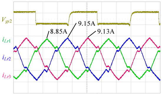
Figure 23.
50% load current statement of three resonant inductors. (Time: 2 µs/div; Vgs2: 10 V/div; iLr1: 5 A/div; iLr2: 5 A/div; iLr3: 5 A/div).
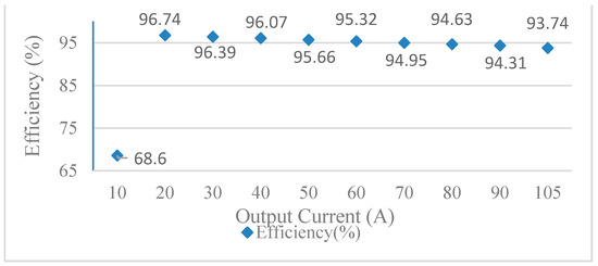
Figure 24.
Efficiency of three-phase wye–delta LLC.
Figure 25 shows the real dimension of the prototype. The height of the circuit is less than 4 cm, and the total area of the circuit is approximately 520 cm2.
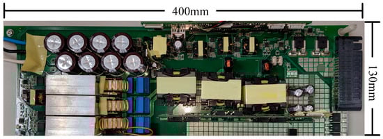
Figure 25.
Three-phase wye–delta LLC prototype.
5. Conclusions
The core of this paper is to propose a complete analysis method for three-phase wye–delta LLC design and application. The methods include circuit operation, time domain analysis, frequency domain analysis, and state–plane analysis. In addition, this paper uses PSIM simulation to verify the accuracy of the analysis. These analysis methods can also be applied to other three-phase resonant topologies, such as three-phase wye–wye LLC.
Finally, this paper realizes a three-phase wye–delta LLC prototype. The input voltage is 380 V, the output voltage/current is 48 V/105 A, and the peak efficiency is 96.57%.
Author Contributions
Supervision, J.-Y.L.; Writing—Original Draft, C.-T.C.; Writing—Review, K.-H.C.; Writing—Review & Editing, Y.-F.L. All authors have read and agreed to the published version of the manuscript.
Funding
This research received no external funding.
Data Availability Statement
I confirm to exclude this statement.
Conflicts of Interest
The authors declare no conflict of interest.
Appendix A
Initial Value Calculation of Resonant Capacitor, Resonant Inductor and Magnetizing Inductor
Definition: when :
When :
When :
When :
When :
References
- Lee, J.B.; Kim, J.K.; Baek, J.I.; Kim, J.H.; Moon, G.W. Resonant Capacitor On/Off Control of Half-Bridge LLC Converter for High-Efficiency Server Power Supply. IEEE Trans. Ind. Electron. 2016, 63, 5410–5415. [Google Scholar] [CrossRef]
- Kodoth, R.; Harikrishnan, T.; Bharath, K.R.; Kanakasabapathy, P. Design and Development of a Resonant Converter Adapted to Wide Ouput Range in EV Battery Chargers. In Proceedings of the 3rd IEEE International Conference on Recent Trends in Electronics, Information & Communication Technology (RTEICT), Bangalore, India, 18–19 May 2018. [Google Scholar]
- Lin, R.L.; Wang, Y.C.; Huang, P.N. Small-Signal Model of LLC LED Driver. In Proceedings of the 2018 IEEE Industry Applications Society Annual Meeting (IAS), Portland, OR, USA, 23–27 September 2018; pp. 1–5. [Google Scholar]
- Wei, Y.; Mantooth, A. An LLC Topology Suitable for Renewable Energy System Applications. In Proceedings of the 2020 IEEE 1st China International Youth Conference on Electrical Engineering (CIYCEE), Wuhan, China, 1–4 November 2020; pp. 1–7. [Google Scholar]
- Hsieh, H.I.; Huang, T.H.; Shih, S.F. An inductive wireless charger for electric vehicle by using LLC resonance with matrix ferrite core group. In Proceedings of the 2015 IEEE Applied Power Electronics Conference and Exposition (APEC), Charlotte, NC, USA, 15–19 March 2015; pp. 1637–1643. [Google Scholar]
- Kundu, U.; Yenduri, K.; Sensarma, P. Accurate ZVS analysis for magnetic design and efficiency improvement of full-bridge LLC resonant converter. IEEE Trans. Power Electron. 2017, 32, 1703–1706. [Google Scholar] [CrossRef]
- Bo, Y.; Lee, F.C.; Zhang, A.J.; Guisong, H. LLC Resonant Converter for Front End DC/DC Conversion. In Proceedings of the APEC 2002, Dallas, TX, USA, 10–14 March 2002; Volume 2, pp. 1108–1112. [Google Scholar]
- Zeng, J.; Zhang, G.; Yu, S.S.; Zhang, B.; Zhang, Y. LLC resonant converter topologies and industrial applications—A review. Chin. J. Electr. Eng. 2020, 6, 73–84. [Google Scholar] [CrossRef]
- Grenier, M.; Aghdam, M.H.; Thiringer, T. Design of on-board charger for plug-in hybrid electric vehicle. In Proceedings of the 5th IET International Conference on Power Electronics, Machines and Drives (PEMD 2010), Brighton, UK, 19–21 April 2010; p. 152. [Google Scholar]
- Deng, J.; Li, S.; Hu, S.; Mi, C.C.; Ma, R. Design methodology of LLC resonant converters for electric vehicle battery chargers. IEEE Trans. Veh. Technol. 2014, 63, 1581–1592. [Google Scholar] [CrossRef]
- Hu, Z.; Qiu, Y.; Liu, Y.F.; Sen, P.C. A control strategy and design method for interleaved LLC converters operating at variable switching frequency. IEEE Trans. Power Electron. 2014, 29, 4426–4437. [Google Scholar] [CrossRef]
- Kim, B.C.; Park, K.B.; Kim, C.E.; Moon, G.W. Load sharing characteristic of two-phase interleaved LLC resonant converter with parallel and series input structure. In Proceedings of the 2009 IEEE Energy Conversion Congress and Exposition, San Jose, CA, USA, 20–24 September 2009; pp. 750–753. [Google Scholar]
- Orietti, E.; Mattavelli, P.; Spiazzi, G.; Adragna, C.; Gattavari, G. Current sharing in three-phase LLC interleaved resonant converter. In Proceedings of the 2009 IEEE Energy Conversion Congress and Exposition, San Jose, CA, USA, 20–24 September 2009; pp. 1145–1152. [Google Scholar]
- Junkai, L.; Ge, Y.; Liu, M.; Yang, Y.; Wu, Q.; Cheng, Z. Research on a New Control Strategy for Reducing Hard-switching Work Range of the Three-phase Interleaved LLC Resonant Converter. In Proceedings of the 2018 IEEE International Telecommunications Energy Conference (INTELEC), Turino, Italy, 7–11 October 2018; pp. 1–6. [Google Scholar]
- Jacobs, J.; Thommes, M.; De Doncker, R.W.A.A. A transformer comparison for three-phase single active bridges. In Proceedings of the 2005 European Conference on Power Electronics and Applications, Dresden, Germany, 11–14 September 2005; p. 10. [Google Scholar]
- Oliveira, D.S.; Antunes, F.L.; Silva, C.E. A three-phase ZVS PWM DC–DC converter associated with a double-wye connected rectifier, delta primary. IEEE Trans. Power Electron. 2006, 21, 1684–1690. [Google Scholar] [CrossRef]
- Hu, S.; Li, Y.; Zhang, Z.; Xie, B.; Chen, M.; Kubis, A. A wye-delta multi-function balance transformer based power quality control system for single-phase power supply system. In Proceedings of the 2015 International Conference on Electrical Systems for Aircraft, Railway, Ship Propulsion and Road Vehicles (ESARS), Aachen, Germany, 3–5 March 2015; pp. 1–7. [Google Scholar]
- Lu, B.; Liu, W.; Liang, Y.; Lee, F.C.; Van Wyk, J.D. Optimal design methodology for LLC resonant converter. In Proceedings of the Twenty-First Annual IEEE Applied Power Electronics Conference and Exposition, 2006, APEC’06, Dallas, TX, USA, 19–23 March 2006; p. 6. [Google Scholar]
- Ryu, S.H.; Lee, B.K. Highly accurate analysis method for LLC dc–dc converters with an improved transformer circuit model. Electron. Lett. 2015, 51, 928–930. [Google Scholar] [CrossRef]
- Liu, J.; Zhang, J.; Zheng, T.Q.; Yang, J. A modified gain model and the corresponding design method for an LLC resonant converter. IEEE Trans. Power Electron. 2017, 32, 6716–6727. [Google Scholar] [CrossRef]
- Fang, X.; Hu, H.; Shen, Z.J.; Batarseh, I. Operation mode analysis and peak gain approximation of the LLC resonant converter. IEEE Trans. Power Electron. 2012, 27, 1985–1995. [Google Scholar] [CrossRef]
- Hu, Z.; Wang, L.; Wang, H.; Liu, Y.F.; Sen, P.C. An accurate design algorithm for LLC resonant converters—Part I. IEEE Trans. Power Electron. 2016, 31, 5435–5447. [Google Scholar] [CrossRef]
- Batarseh, I.; Lee, C.Q. State-plane analysis of high order parallel resonant converters. In Proceedings of the 34th Midwest Symposium on Circuits and Systems, Monterey, CA, USA, 14–17 May 1992; pp. 939–942. [Google Scholar]
- Feng, W.; Lee, F.C. Optimal trajectory control of LLC resonant converters for soft start-up. IEEE Trans. Power Electron. 2014, 29, 1461–1468. [Google Scholar] [CrossRef]
Publisher’s Note: MDPI stays neutral with regard to jurisdictional claims in published maps and institutional affiliations. |
© 2021 by the authors. Licensee MDPI, Basel, Switzerland. This article is an open access article distributed under the terms and conditions of the Creative Commons Attribution (CC BY) license (https://creativecommons.org/licenses/by/4.0/).