Article

Voltage Profile and Sensitivity Analysis for a Grid Connected Solar, Wind and Small Hydro Hybrid System

1
African Centre of Excellence in Energy and Sustainable Development, University of Rwanda, Kigali P.O. Box 4285, Rwanda
2
Department of Electrical and communications Engineering, School of Engineering, Moi University, Eldoret P.O. Box 3900-30100, Kenya
3
Department of Electrical Engineering, Tshwane University of Technology, Pretoria X680-0001, South Africa
*
Author to whom correspondence should be addressed.
Energies 2021, 14(12), 3555; https://doi.org/10.3390/en14123555
Submission received: 5 May 2021 / Revised: 25 May 2021 / Accepted: 26 May 2021 / Published: 15 June 2021
(This article belongs to the Topic Innovative Techniques for Smart Grids)

Abstract

:
Due to increase in integration of renewable energy into the grid and power quality issues arising from it, there is need for analysis and power improvement of such networks. This paper presents voltage profile, Q-V sensitivity analysis and Q-V curves analysis for a grid that is highly penetrated by renewable energy sources; solar PV, wind power and small hydro systems. Analysis is done on IEEE 39 bus test system with Wind power injection alone, PV power injection alone, with PV and wind power injection and with PV, wind and micro hydro power injection to the grid. The analysis is used to determine the buses where voltage stability improvement is needed. From the results, it was concluded that injection of the modeled wind power alone helped in stabilizing the voltage levels as determined from voltage profiles and reactive power margins. Replacing some of the conventional sources with PV power led to reduction of voltages for weak buses below the required standards. Injection of power from more than one renewable energy source helped in slightly improving the voltage levels. Distribution Static compensators (D-STATCOMs) were used to improve the voltage levels of the buses that were below the required standards.

1. Introduction

The demand for electric energy is rapidly increasing and putting pressure on utilities to expand their generation. This coupled with the need for clean energy has led to energy demand growth. Because of this, the researchers are envisaging the power generation technique from the renewable energy sources such as solar, hydro and wind. These energy sources are preferred for distributed generation because of their abundance, cleanliness and low cost [1,2]
Solar PV and Wind power systems are getting popular because of their availability and reducing cost. However, they are intermittent in nature [3,4,5,6] and cannot satisfy power requirements alone throughout the year. Small hydro systems are also getting interest to generate electrical power in remote areas. The limitation to small hydro power is its poor voltage and frequency regulation. Therefore, a reliable technique is required to maintain constant voltage and frequency irrespective of the load and load types [7].
Grid interconnection of these renewable energy sources come with many advantages such as [8,9,10]:
  • Less environmental pollution because of increased use of non- polluting generation sources.
  • Low cost because of non- consumption of fuel.
  • The power capacity of connected grids increase to meet the increase in demand.
  • Improved supply security.
  • Cheaper power for consumers due to increase in power supply from cheaper sources.
Photovoltaic (PV) can generate electricity from readily available sunlight [11]. This power can either be utilized in stand-alone mode of connected to the grid. Significant increase in PV generation connected to the grid present technical challenges and major impacts on system stability due to its stochastic nature [12]. Literature [13] analyzes voltage stability of a power system using P-V curves. In [12,14] the effects of photovoltaic integration at different levels is analyzed. Literature [15] discusses the effects of high penetration of PV power on voltage stability of a network. It also analyzes the effects on voltage levels when the connected PV power is lost due to shading of PV panels by movement of clouds. It also proposes the use of D-STATCOM to compensate for instability.
There is a high growth of wind power generation which is estimated to reach 20% of the total generation by the year 2040 [16,17]. The mostly used generator in wind farms is the doubly fed induction generators [18]. Due to the intermittency of wind power and the reactive power consumption of DFIG, the effects of integration of wind farms into the grid cannot be neglected [19,20]. Integration of small amounts of wind power while maintaining the conventional sources can help in voltage support as found in [21]. Serious problems on voltage stability and power quality arise due to wind farm integration with the grid on large scales [22].
The majority of power used worldwide is from hydro power plants; up to 20% of the total power [8,23]. However this power comes from large hydro power plants that require huge amounts of land for water reservoirs and dams and usually cause environmental effects. This has led to increased research on small hydro power plants that operate on run-off rivers which do not require any reservoirs [24,25]. Small hydro power plants can handle peak load demand easily with less cost compared to their conventional generating plants due to the slow start-up and operational needs of the latter [26,27]. The increase in grid interconnection of micro-hydro power plants in the recent past is due to their excellent performance and benefits such as high efficiencies (70–90%), high capacity factors (greater than 50%) and low output power variations [8,28,29,30].
Voltage stability is one of the main challenges that come up with grid interconnection of intermittent renewable energy sources. Voltage stability can be divided into static or dynamic. Dynamic voltage stability is based on differential equations that determine the variation of bus voltages with varying system operating parameters. The methods used in analyzing the dynamic voltage stability include bifurcation analysis, small signal stability analysis, time domain simulations and energy function method [31,32,33,34]. Static voltage stability is based on power flow equations and can point out the mechanisms of voltage collapse for different operating conditions. This method takes less computational time and yields most of the required information concerning voltage stability of the system [35]. Since the system dynamics that influence voltage stability are slow, many aspects can be analyzed by use of static methods which determine the viability of equilibrium point represented by a given operation of the power system [36]. The methods used in static voltage analysis include; Q-V curves, bus sensitivities and P-V curves [35].
Due to the effects on power quality arising from connection of these renewable energy sources to the grid, several mitigation methods have been used in literature. Flexible AC transmission systems (FACTS) have been used to improve voltage profile in grids affected by connection of renewable energy sources. FACTS refers to a family of power electronic devices that can control the flow of active and reactive powers [37,38]. These FACTS devices can either provide series compensation or shunt compensation. Series compensation devices include Thyristor controlled series capacitor (TCSC), Thyristor controlled phase shift transformer (TCPST) and static synchronous series compensator (SSSC) [39] while the commonly used shunt compensators include fixed or variable capacitors [39,40] static compensators (STATCOMs) and static VAR compensators (SVCs). Literatures [41,42] review the use of dynamic voltage restorer (DVR) and STATCOMs in compensating voltage swells and sags. The combination of the DVR and STATCOM forms unified power quality compensator (UPQC) where DVR is used to supply series voltage in the event of voltage sag or swell while STATCOM is used to supply or absorb reactive power to maintain constant DC-link voltage.
Distribution FACTS devices are popularly used nowadays because they are smaller and less expensive than conventional FACTS devices [43,44]. STATCOM devices were used by [4,45] to support reactive power demand and improve voltage profile for a wind integrated grid. The performance of FACTS devices is done in literature [41]. Literature [42] compares the performance of STATCOM and SVC in improvement of the voltage profile after wind power integration. STATCOM is concluded to give better performance than SVC.
This paper analyzes the effects of connecting three renewable energy sources (solar PV, Wind and micro hydro) to the grid voltage levels. The sensitivities of the grid buses are also analyzed. A method for mitigating these effects is implemented and conclusions made. Solar PV system was connected to the grid through voltage source inverter to convert the DC power to AC power. Wind power was connected to the grid through voltage source converters, one to convert wind power from AC to DC for ease of control mechanisms and the other from DC to AC because the grid used was AC. Small hydro system was connected directly to the grid system.
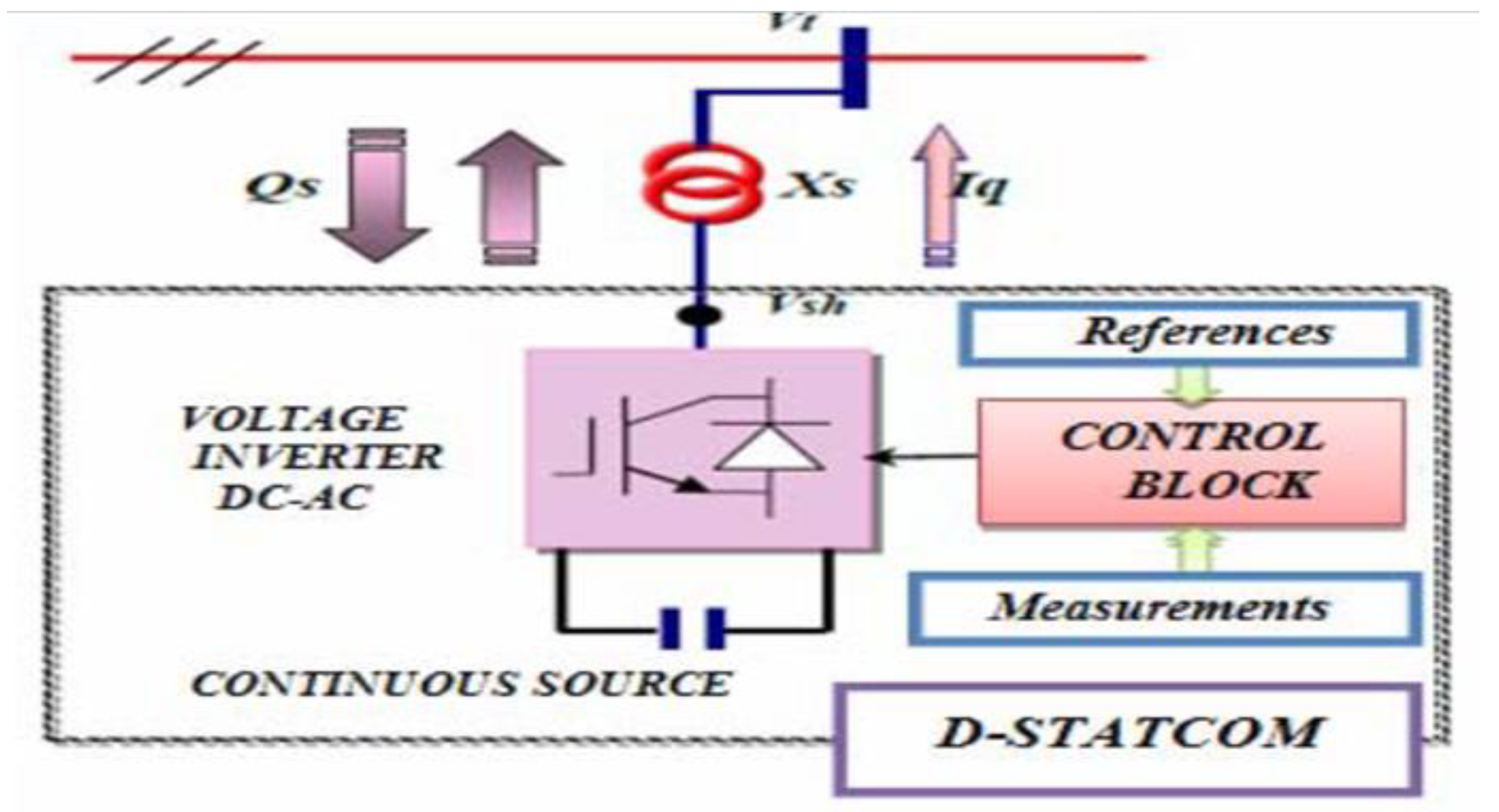
Due to the effects of these renewable energy sources on the grid voltages and bus sensitivities, distribution static compensator (D-STATCOM) devices were connected to the affected grid buses in order to ensure the voltage levels are within the required standards as stated in IEEE standards. According to this standard, the voltage levels should always be within 5% above or below the nominal voltage value [46].
Figure 1 show the three renewable energy sources connected to the grid.

2. Mathematical Mode

2.1. Solar PV

The equivalent circuit of a PV cell is shown in Figure 2 [47].
The current source Iph represents the cell photocurrent. Rsh and Rs are the intrinsic shunt and series resistances of the cell, respectively. Usually the value of Rsh is very large and that of Rs is very small, hence they may be neglected to simplify the analysis [48]. Practically, PV cells are grouped in larger units called PV modules and these modules are connected in series or parallel to create PV arrays which are used to generate electricity in PV generation systems. The equivalent circuit for PV array is shown in Figure 3 [49].
The voltage–current characteristic equation of a solar cell is provided in [50]:
Module photo-current Iph:
I p h = [ I s c + K i ( T 298 ) ] I r 1000 I p h
where: I p h = photo-current in Amperes, I s c = short circuit current in Amperes, Ki = short-circuit current of cell at 25 °C and 1000 W/m2, T = operating temperature in Kelvin, I r = solar irradiation (W/m2).
Module reverse saturation current Irs:
I r s = I s c [ exp ( q V O C / N s K n T ) 1 ]
where: q = electron charge, = 1.6 × 10⁻¹⁹ C; Voc = open circuit voltage (V); Ns = number of cells connected in series; n: the ideality factor of the diode; K: Boltzmann’s constant, =1.3805 × 10⁻²³ J/K.
The module saturation current I0 varies with the cell temperature, which is given by:
I 0 = I r s [ T T r ] 3 exp [ q E g 0 n k ( 1 T 1 T r ) ]
where: T r = nominal temperature = 298.15 K; Eg0 = band gap energy of the semiconductor = 1.1 eV; The current output of PV module is:
I = N p I p h N p I 0 [ exp V / N s + I R s / N p n V t 1 ] I s h
with
V t = k T q
and
I s h = V N p / N s + I R s R s h
where: N p = number of PV modules connected in parallel; R s = series resistance (Ω); R s h = shunt resistance (Ω); V t = diode thermal voltage (V).
The output power of PV panels depends on the current produced due to irradiation of solar rays on the module. Thus the output power can be written as a function of insolation which is the power produced per unit square meter of the panel. Considering panels of size 1 m2, total power is the product of insolation, number of panels and the efficiency of the panel to effectively convert the solar irradiation into electric power. Thus the output power of PV panels can be mathematically expressed as:
P s = η I S n
where: η = energy conversion efficiency, I = Current produced due to irradiation and S n = generating power per 1 m2 for 1 MJ/m2.
In this paper, three PV systems were modeled with the aim of replacing three conventional generators in the IEEE 39 bus system. The PV parameters are shown in Table 1.

2.2. Doubly Fed Induction Generator (DFIG) for Wind Power

DFIGs have separate active and reactive control mechanism, hence they are the mostly used generators in wind farms as more than 85% of wind turbines utilize them. Furthermore, DFIG’s converter rating is only 30% of the total generator rating which makes it attractive in the economic point of view [51,52]. The stator voltage and flux of a DFIG can be expressed as [53];
V s = R s I s + d ψ s d t ψ s = L s I s + L m I r
where Vs is the stator voltage, R s = stator winding resistance, I s is the stator current, ψ s is the stator flux linkage, L s is the stator inductance, L m is the maximum mutual inductance and I r is the rotor current.
The rotor voltage ( V r ) and rotor flux ( ψ r ) are given by;
V r = R r I r + d ψ r d t j ω m ψ r ψ r = L r I r + L m I s
where ωm is the rotor mechanical speed and Lr is the rotor inductance.
From Equations (8) and (9), the following expressions can be obtained:
d I s d t = L r R s + j ω m L 2 m L r L s L 2 m I s j ω m L r L m L m R r L r L s L m 2 I r + L r L r L s L m 2 V s L m L r L s L m 2 V r d I r d t = L m R s + j ω m L m L s L r L s L 2 m I s j ω m L r L s L s R r L r L s L m 2 I r + L m L r L s L m 2 V s L s L r L s L m 2 V r
The magnitudes and parameters are all referred to the stator [53]. The angular stator frequency and rotor frequency are related by:
ω r = ω s ω m
where ω r is the rotor electrical speed and ω s is the electric synchronous speed.
The rotor and stator voltages in the stationary reference frame are given by:
V r = R r I r + s j ω s L σ r I r + s j ω s L m ( I r + I s ) V s = R r I s + s j ω s L σ r I s + s j ω s L m ( I r + I s )
where L σ r is the rotor leakage inductance?
The three phase active power losses for the stator ( P s ) and rotor ( P r ) of the DFIG machine are given by;
P s ( l o s s e s ) = 3 2 R s I s 2 P r ( l o s s e s ) = 3 2 R r I r 2
The active power for the stator and rotor are given by;
P s = 3 2 Re ( V s I s * ) = 3 2 R s I s 2 + 3 2 ω s L m Re ( j ( I r I s * ) ) P r = 3 2 Re ( V r I r * ) = 3 2 R r I r 2 + 3 2 s ω s L m Re ( j ( I r I s * ) )
The mechanical power of DFIG is given by;
P m e c = P s + P r P s ( l o s s e s ) P r ( l o s s e s ) = 3 2 ω s L m Re [ j ( I r I s * ) + ( s I s I r * ) ]
The parameters used in modeling the DFIG are shown in Table 2.

2.3. Small Hydro System

The hydraulic power from a hydro system is given by [54];
P h = g ρ W H   watts
where W = water discharge through the turbine in m/s, ρ = density in Kg/m3, H = Head in meters and g = gravitational acceleration = 9.81 m/s2.
Since the density of water is 1000 Kg/m3 then the power is given by;
P h = 9.81 W H   kilowatts
Total potential of water can be calculated from;
P t o t a l = P h n t n g   kW
where: P h is the hydraulic power, n t is the turbine efficiency and n g is the generator efficiency.

2.4. Voltage Stability

Voltage stability analysis can be done using time simulations that capture the events that lead to instability or by use of static methods that examine the viability of a balance point that is represented by specified parameters of the power system. There are 4 static methods for voltage stability analysis: V-Q Sensitivity Analysis, Q-V Modal Analysis, V-Q Curves and P-V Curves. These static analysis methods allow examination of a wide range of system conditions can provide information about the nature of the problem and can identify the key contributing factors [55].
This paper utilizes the static methods to assess the effects of connecting solar PV, wind power and small hydro into the grid.

2.4.1. Q-V Sensitivity Analysis

This method calculates the relationship between voltage change and reactive power change [56];
Δ U = J R 1 Δ Q
where: Δ U = incremental change in bus voltage magnitude (vector), Δ Q = incremental change in bus reactive power injection (vector), J R = reduced Jacobian matrix.
The V-Q sensitivities are found from the elements of the inverse of the reduced Jacobian matrix J R while the diagonal components are the self-sensitivities given by;
U i Q i
The non-diagonal elements are the mutual sensitivities
U k Q i
The sensitivities of voltage controlled buses are equal to zero since their voltages are assumed to be constant. V-Q sensitivities can either be; Positive or negative. Positive sensitivities shows that the system is under stable operation, the smaller the sensitivity, the more stable the system. As stability decreases, the magnitude of the sensitivity increases, becoming infinite at the stability limit. Negative sensitivities show unstable operation. At this region, the system is uncontrollable.

2.4.2. Q-V Modal Analysis

This modal analysis approach provides more information regarding the mechanism of instability. Voltage stability characteristics of the system are identified by determining the eigenvalues and eigenvectors of the reduced Jacobian matrix J R [56].
J R = ξ i Λ η
where: Λ = diagonal eigenvalue matrix, ξ = right eigenvector matrix, η = left eigenvector matrix, ξ i = the ith right eigenvector, ith column of right eigenvector matrix, η i = is the ith left eigenvector, ith row of left eigenvector matrix.
Using modal analysis techniques Equation (19) becomes;
u = Λ 1 q
where: u = η Δ U is the vector of modal voltage variations, q = η Δ Q q = η ΔQ is the vector of modal reactive power variations.
The inverse transformation of (23) is given by;
Δ U = ξ u Δ Q = ξ q
For U-Q modal analysis, Positive eigenvalue shows that the system is voltage stable. The smaller the magnitude, the closer the ith modal voltage is to being unstable. The magnitude of the eigenvalues can provide a relative measure of the proximity to instability. Zero eigenvalue shows that the ith modal voltage collapses because any change in that modal reactive power causes infinite change in the modal voltage. Negative eigenvalue shows that the system is voltage unstable. Zero reactive power is assumed for buses without load elements.
Bus participation factors give the relative participation of a bus in a certain mode. They are used to determine voltage weak areas or unstable (not controllable) areas. The sum of all the bus participations for each mode is equal to unity. The size of bus participation in a given mode indicates the effectiveness of remedial actions applied at that bus in stabilizing that mode [56].

2.4.3. Q-V Curves

Reactive-Voltage (Q-V) curve is one of the methods used in determining the stability of an electrical system. From Q-V curves, reactive power margin is measured as a distance between the lowest MVAr point and Voltage axis as shown in Figure 4 [57].
Therefore, reactive power margin indicates how further the loading on a particular bus can be increased before its loading limit is exhausted and voltage collapse takes place [58]. Literature [59] used reactive power margins to evaluate voltage instability problems for coherent bus groups. These margins are based on the reactive reserves on generators, SVCs and synchronous condensers that exhaust reserves in the process of computing a Q-V curve at any bus in a coherent group or voltage control area. This paper uses Q-V curves to analyze how the reactive power margins change with integration of different renewable energy sources to the grid.

2.5. Distribution Static Compensator (D-STATCOM)

D-STATCOM is a static synchronous generator operating as a Static Var Compensator (SVC) connected in parallel with the output current (capacitive or inductive) that can be controlled independently of the AC voltage network. The principle functions of a D-STATCOM are to mitigate the impact of voltage dips and voltage peaks of sensitive loads, voltage regulation, harmonic compensation and reactive power control. Its function in compensating reactive power and therefore regulating the bus bar voltage where it is connected is applied in this research paper. The basic structure for a static compensator is depicted in Figure 5 [60,61].
The voltage of D-STATCOM, V s h is injected in phase with the line voltage Vt, and in this case there is no exchange of energy with the active network, but only reactive power to be injected (or absorbed) by the D-STATCOM.
The reactive power exchange with the network is done by varying the amplitude of the output voltages [61].
The output voltage of the gate turn-off thyristor (GTO) converter ( V s h ) is controlled in phase with the system voltage ( V t ). The output current of the D-STATCOM ( I q ) varies depending on V s h [61]. If V t < V s h then the phase angle of I q is leading with respect to the phase angle of V t by 90 degrees. This leads to reactive power flowing from the D-STATCOM (capacitive mode). When V t > V s h then the phase angle of I q is lagging with respect to V t by 90 degrees; the D-STATCOM consumes reactive power. When V t = V s h then no reactive power is delivered to the power system. As a result, lagging reactive power flows into the D-STATCOM (inductive mode).
The amount of the reactive power is proportional to the voltage difference between V t and V s h . The variation of the output voltages amplitude is achieved by varying the direct voltage across the capacitor. The D-STATCOM can deliver a capacitive or inductive current independent of the network voltage. So it can provide the maximum capacitive current even at low voltage values. Its ability to support the supply voltage is better than the SVC.
The advantage of this device is in its ability to exchange energy nature (capacitive or inductive) only with an inductor. Unlike SVC, there is no capacitive element that can cause resonances with inductive elements of the network. The structure and operational characteristic is shown in Figure 6. The D-STATCOM smoothly and continuously controls voltage from V 1 to V 2 . However, if the system voltage exceeds a low-voltage ( V 1 ) or high voltage limit ( V 2 ), the D-STATCOM acts as a constant current source by controlling the converter voltage ( V 1 ) appropriately [61].
The equivalent circuit for D-STATCOM is shown in Figure 7.
Taking V s h ¯ = V s h δ s h as the reference phase and the fundamental component of the voltage source converter as V s ¯ = V s 0 . The active and reactive power exchanged with the bus is given by;
P = V s h V s X t sin δ s h Q = V s 2 X t V s h V s X t cos δ s h
The current injected to the busbar by the STATCOM is given by;
I s h = V s h V t j X t
When all the quantities are in three phase;
V ¯ = [ V a V b V c ] ,   V s h ¯ = [ V a s h V b s h V c s h ] , I s h ¯ = [ I s h a I s h b I s h c ]
The power injected to the busbar is given by;
S ¯ = V s h ¯ I s h ¯ = V t ¯ ( V s h * ¯ V t * ¯ ) j X t = V t ¯ V s h ¯ V t 2 ¯ j X t
The active and reactive power injected by the D-STATCOM is given by;
P s h = V t V s h sin ( θ t θ s h ) Q s h = V t ( V s h cos ( θ t θ s h ) V t ) / X t

2.6. Sizing and Placement of D-STATCOM

There are various criteria for determining the required size of STATCOM devices [62] and [63]. STATCOM devices can be sized considering the ratings of the renewable energy systems connected to the gridas presented in [64]. In this study, the amount of reactive power needed for compensation is assumed to be equal to the sum of Wind turbine systems, PV systems and Small hydro systems ratings’ depending on which one is integrated at a given time. Table 3 shows STATCOM sizes connected for different connections of renewable energy types.
Literature [65] made comparisons of placement of STATCOM devices at the weakest buses of a network. The comparison is made on aggregated placement and dispersed placement at the weakest buses. The dispersed placement is preferred over the aggregated placement since it results to both lowest power losses and increase loadability of the network. Thus, considering this, this paper places the designed STATCOM devices on the weakest buses of the IEEE 39 bus test grid to improve the voltage stability with influx of the power from the renewable energy sources.

3. Simulation and Results

After modeling the three renewable energy sources (Solar PV, wind and small hydro) their powers were injected into the IEEE 39 bus system for analysis of voltage profile, V-Q sensitivities and Q-V curves. Firstly, wind power was injected at bus 12 (15 MW) and bus 28 (15 MW) and analysis done. Secondly, three generators of the test system were replaced by solar power with varying insolation (from 1 kW/m2 to 0.7 kW/m2) at bus 30 (80 MW), at bus 32 (60 MW) and at bus 38 (100 MW) and analysis done. Thirdly, analysis was done with penetration of both wind power and solar power. Lastly, a small hydropower (10 MW) was injected at bus 03 and analysis done when the system is penetrated by all the three; solar power, wind power and small hydro power.
In order to improve the voltage levels to the required standards, the modeled D-STATCOM was connected to buses 12 and 07 and the results analyzed in comparison with those before compensation.
The IEEE 39 bus test system used in this work is shown in Figure 8.

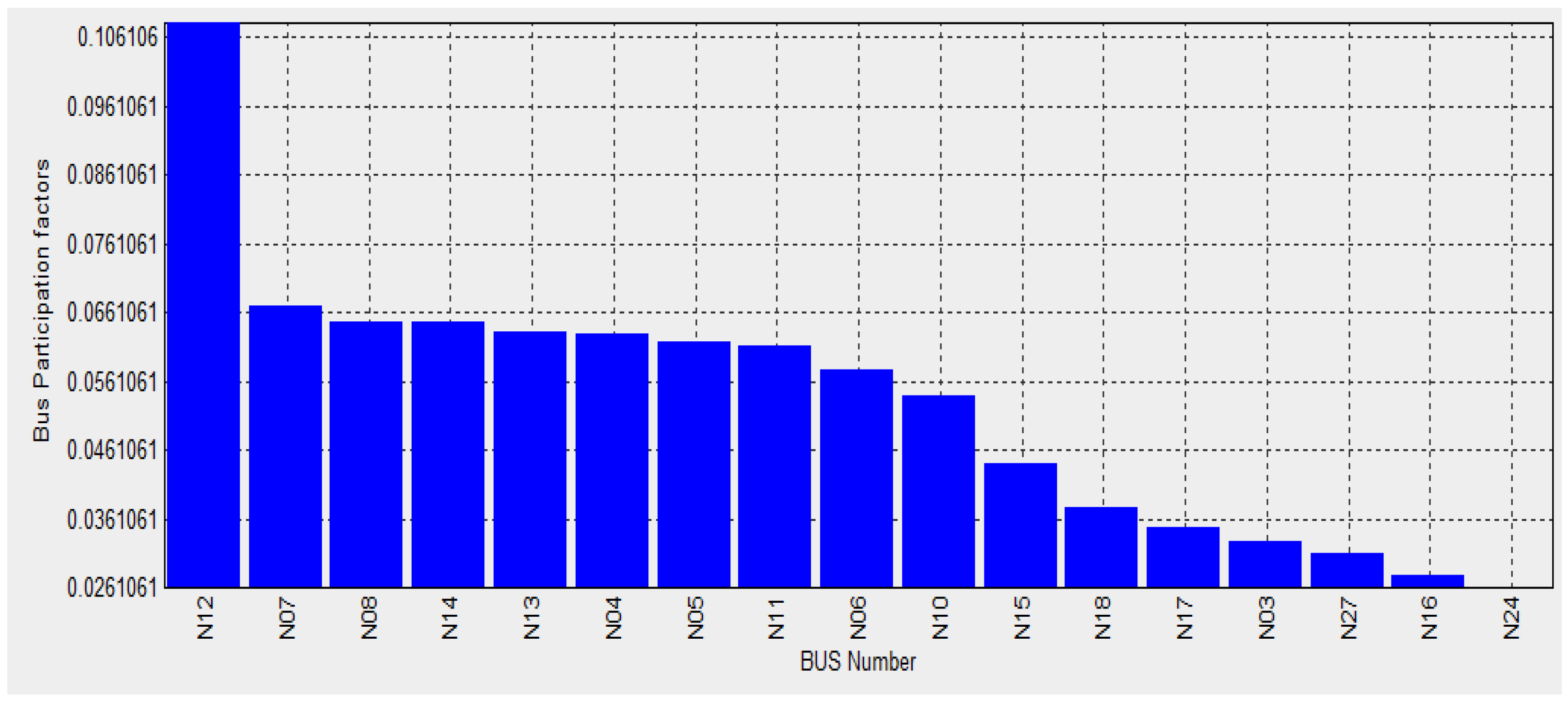
3.1. Weak Buses of the IEEE 39 Bus System

The weakest buses of the IEEE 39 test bus system were determined using bus participation factors and are shown in Figure 9. The weakest buses are buses 12, 07 and 08.

3.2. Voltage Profile

3.2.1. Voltage Profile before Varying Reactive Power
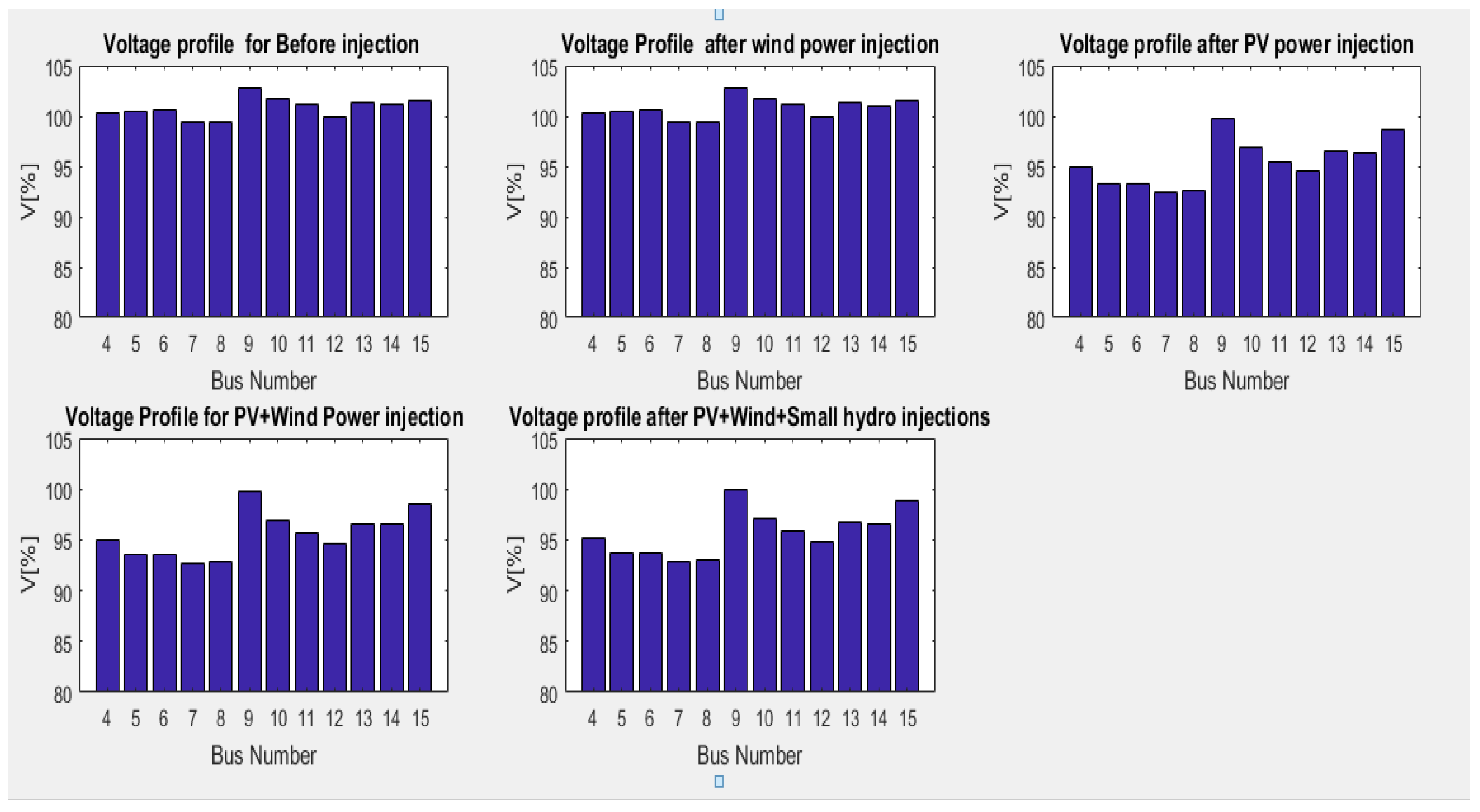
Table 4 and Figure 10 (considering the weak buses of the system) show the voltage profile of the IEEE 39 bus system before injecting any of the modeled systems into it, when wind power is injected at buses 12 and 28, when solar PV power alone is injected into buses 30, 32 and 38, when both solar power(injected at buses 30, 32 and 38) and wind power (injected at buses 12 and 28) and when all the three are injected to the grid; (solar power at buses 30, 32 and 38, Wind power (at buses 12 and 28) and small hydro power (at bus 03). Both Voltage levels and percentage of the nominal voltages are shown in Table 4 while the percentage voltage levels for the weakest buses of the system are depicted in Figure 10.
From the Table 4 and Figure 10, the voltage profile for the weak buses are seen to reduce when the system is penetrated with PV solar power then slightly improve with the connection of wind power and small hydro power into the system. The buses with the highest voltage drops when PV power is used to replace the three IEEE 39 bus test system were, bus 5 from 100.53% to 93.54%, bus 6 from 100.77% to 93.57%, bus 7 from 99.7% to 92.77% and bus 8 from 99.6% to 92.89%. Considering the weakest buses of the system (12 and 07) the voltage levels percentages for bus 12 are seen to change from 100.02% to 99.96% to 94.67% to 94.84% and 94.95% in the presented order while for Bus 07, the voltage profile percentages change from 99.7%, to 99.7% to 92.77% to 92.99% to 93.93% in that order.

3.2.2. Voltage Profile When Reactive Power on Bus 07 Is Varied

The reactive power consumed by the load on bus 07 was varied and voltage profile analyzed. Table 5 and Figure 11, show the voltage profile for the system when the reactive power of the load at bus 07 is increased from 84.0 MVAR to 100.0 MVAR.

3.2.3. Voltage Profile When Reactive Power on Bus 12 Is Varied

The reactive power consumed by the load on bus 07 was varied and voltage profile analyzed. Table 6 shows the voltage profile for the system when the reactive power of the load at bus 07 is increased from 84.0 MVAR to 100.0 MVAR. Figure 12 shows the voltage profile for the weakest buses of the IEEE 39 bus system.
From Table 5 and Table 6 and Figure 11 and Figure 12, there is a reduction in the voltage levels when PV penetrates the grid and the voltage levels improve as wind and small hydro powers are injected to the grid. From Table 5, The buses with the highest voltage drops when PV power is used to replace the three IEEE 39 bus test system were, bus 4 from 100.28% to 94.88%, bus 5 from 100.37% to 93.32%, bus 6 from 100.61% to 93.35%, bus 7 from 99.46% to 92.46% and bus 8 from 99.4% to 92.62%. From Table 6, the buses with the highest voltage drops when PV power is used to replace the three IEEE 39 bus test system were, bus 4 from 100.31 to 94.91, bus 5 from 100.45% to 93.43%, bus 6 from 100.68% to 93.45%, bus 7 from 99.62% to 92.66% and bus 8 from 99.52% to 92.68% and bus 12 99.62% to 94.22%. Considering buses 04 and 05, from Table 5; the voltage levels changed 100.28% to100.26% to 94.86% to 95.04% to 95.16% for bus 04 and from 100.37% to 100.37% to 93.32% to 93.55% to 93.69% for bus 05 respectively. From Table 6 the voltage levels changed from 100.31% to 100.29% to 94.91% to 95.09% to 95.21% for Bus 04 and from 100.45% to 100.44% to 93.43% to 93.65% to 93.78% for bus 05 respectively.

3.3. Q-V Sensitivity Analysis

3.3.1. Q-V Sensitivities before Varying Reactive Power

The bus sensitivities were determined using the standard loads of the IEEE 39 bus system and the results are shown in Table 7.
From Table 7, Q-V sensitivities increase with PV replacement of the conventional sources then start reducing as wind power and small hydro power are connected to the grid. Considering buses 12 and 07; the sensitivities change from 0.0332 to 0.0333 to 0.0369 to 0.0367 to 0.0366 for bus 12 and from 0.0150 to 0.10149 to 0.0191 to 0.0189 to 0.0188 for bus 07 respectively.

3.3.2. Q-V Sensitivities when Reactive Power at Buses 07 Is Varied

The reactive power consumed by the load on bus 07 was varied and bus sensitivities determined. Table 8 shows the bus sensitivities for the system when the reactive power of the load at bus 07 is increased from 84.0 MVAR to 100.0 MVAR.

3.3.3. Q-V Sensitivities when Reactive Power at Buses 12 Is Varied

The reactive power consumed by the load on bus 12 was varied and sensitivities of the buses determined. Table 9 shows the bus sensitivities for the system when the reactive power of the load at bus 12 is increased from 88.0 MVAR to 100.0 MVAR.
From Table 8 and Table 9 the V-Q sensitivities increase when the reactive power is increased compared to those on Table 4. The V-Q sensitivities are highest when PV alone is injected to the grid but reduce with wind and solar penetration. From Table 5, the highest sensitivities change from 0.0332 to 0.0333 to 0.0370 to 0.0368 to 0.0367. From Table 6, the highest sensitivities change from 0.0335 to 0.0336 to 0.0372 to 0.0371 to 0.0370 in that order.
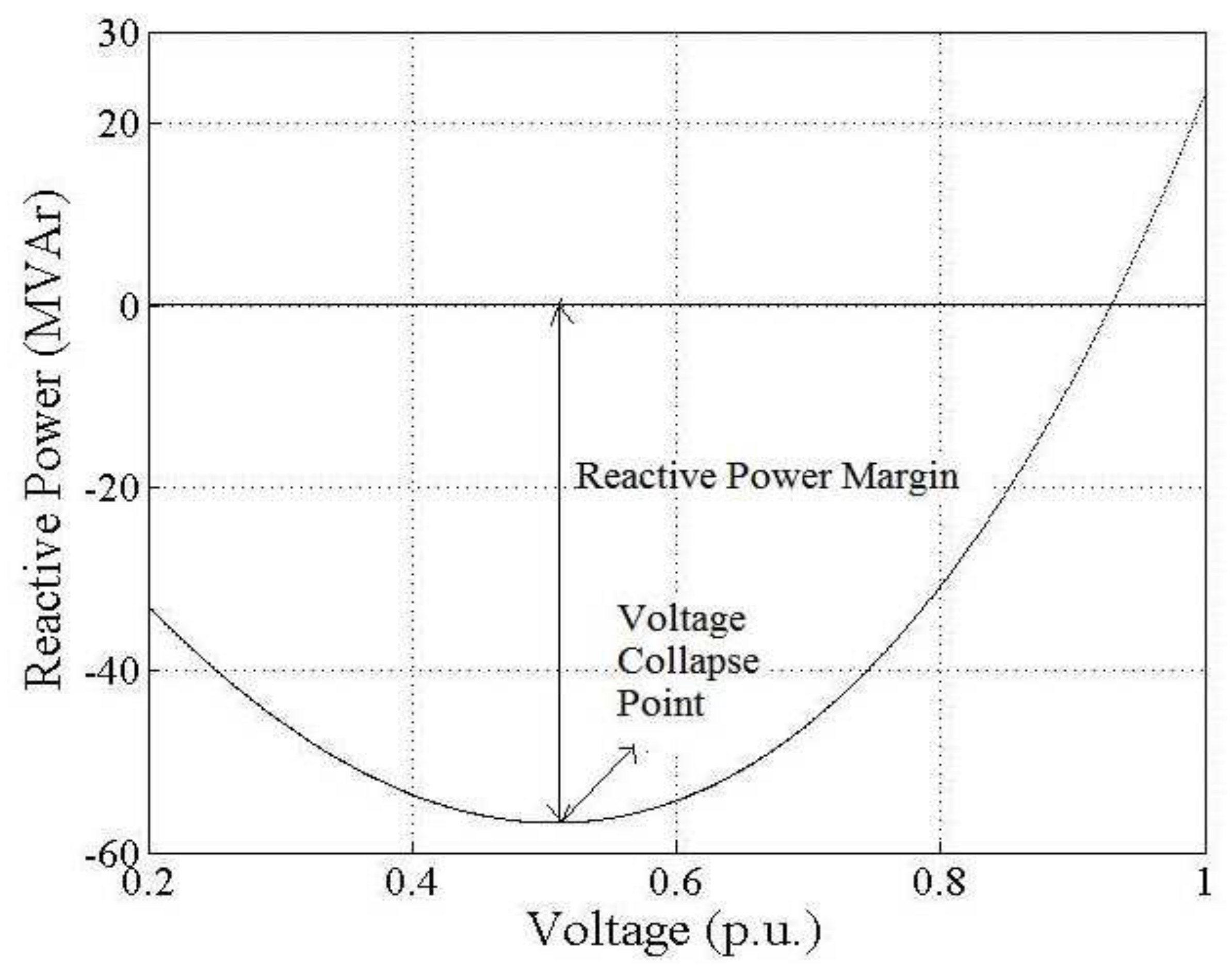
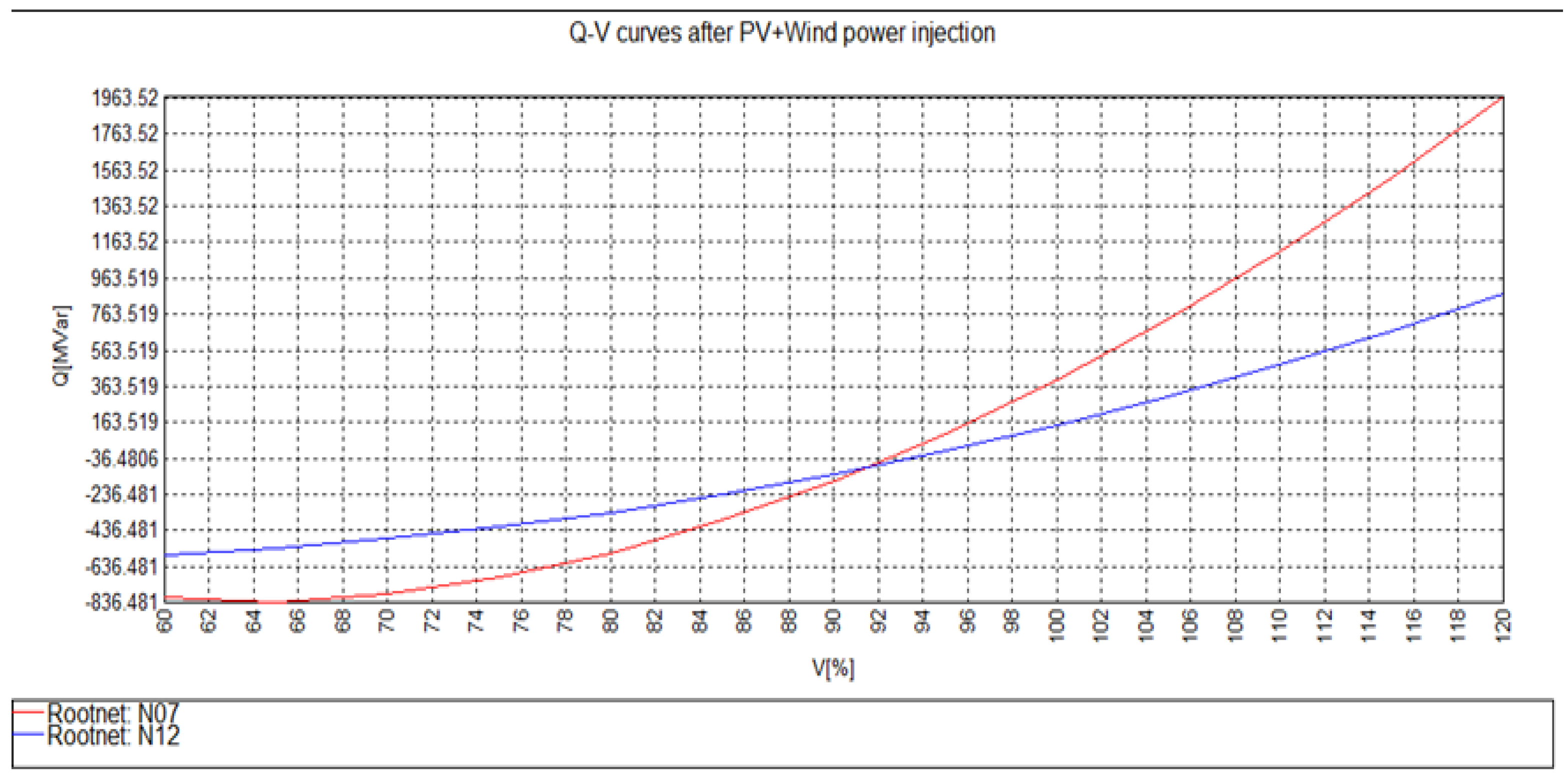
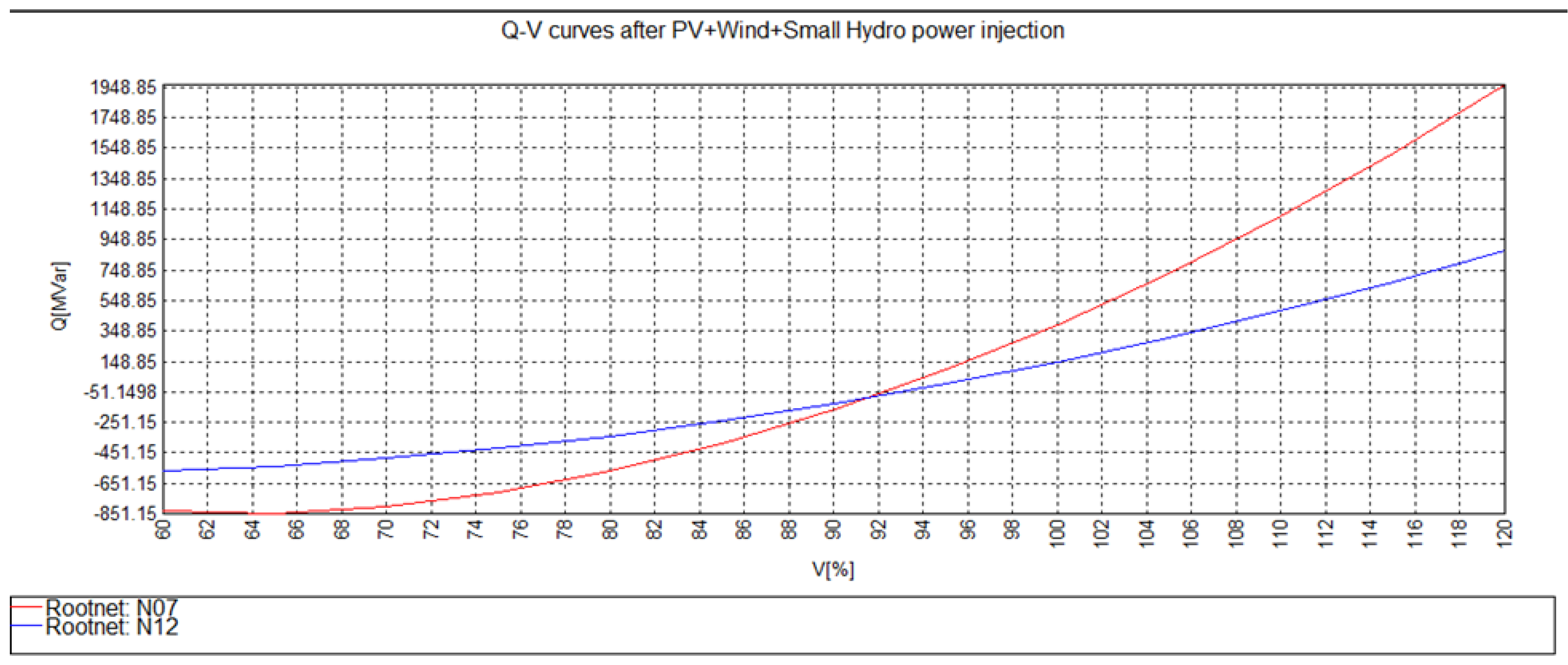
3.4. Q-V Curves

The Q-V curves for the system with standard IEEE 39 parameters, with wind power injection alone, with PV power injection alone, with PV and wind power injection and with PV, wind and small hydro power injections are shown in Figure 13, Figure 14, Figure 15, Figure 16 and Figure 17 respectively
From Figure 13, Figure 14, Figure 15, Figure 16 and Figure 17, considering bus 07, it is noted that the reactive power margins for the system increased with Wind power injection alone from 1530 MVar to 1531 MVar, reduced with PV injection alone (from 1530 MVar to 800 MVar) then increased to 836 MVar for PV + Wind and to 851 MVar PV + Wind + small hydro for bus 07.

3.5. Voltage Profile after Connecting D-STATCOM

3.5.1. Before Varying Reactive Power

Table 10 and Figure 18 show the voltage profile after connecting STATCOM on buses 07 and 12 in order to improve the voltage levels before varying reactive power.

3.5.2. After Varying the Reactive Power on the Load at Bus 07

Figure 19 and Table 11 show the voltage profile of the IEEE 39 bus system when the reactive power of the load at bus 07 is changed from 84 MVar to 100 MVar.

3.5.3. After Varying the Reactive Power on the Load at Bus 12

Table 12 and Figure 20 show the voltage profile of the IEEE 39 bus system when the reactive power of the load at bus 12 is changed from 88 MVar to 100 MVar.
From Table 10, Table 11 and Table 12 and Figure 18, Figure 19 and Figure 20, it can be seen that after connection of D-STATCOM at buses 07 and 12, all the voltage levels of all the buses were in the required standard i.e., within 5% above or below the nominal value for all the three cases; with PV penetration alone, with PV and Wind power penetration and with PV, wind power and small hydro penetration.

4. Conclusions

This paper has dealt with the analysis and mitigation of voltage stability on a grid highly penetrated by power from renewable energy sources. Determination of buses that need mitigation of voltage profile effects after integrating power from different renewable energy sources into IEEE 39 bus system network has been done. This has been done by analyzing voltage profiles, Q-V bus sensitivities and reactive power margins from Q-V curves. D-STATCOM was modeled and used to improve the voltage profiles. From the analysis, it was noted that connection of the modeled wind power alone while maintaining the conventional sources helped in stabilizing the system voltages as seen from the increase in reactive power margis from Q-V curves. When some of the conventional sources were replaced by PV systems the stability of the voltages in the grid was affected. It was further noted that connecting more than one energy source to the grid slightly improves the voltage levels and stability. In order to ensure that all the voltage levels meet the required standards, D-STATCOM was used. After connection of the D-STATCOM, the voltage levels for all the buses were improved to the required standards.

Author Contributions

Conceptualization, N.S.; methodology, N.S.; software, N.S.; validation, N.S., L.K.L. and J.M.; formal analysis, N.S.; investigation, N.S.; resources, N.S.; data curation, N.S.; writing—original draft preparation, N.S.; writing—review and editing, N.S., L.K.L. and J.M.; visualization, N.S.; supervision, L.K.L. and J.M.; project administration, L.K.L. and J.M.; funding acquisition, N.S. All authors have read and agreed to published version of the manuscript.

Funding

This research work was funded by World bank and University of Rwanda through African Centre of Excellence in Energy for sustainable development.

Conflicts of Interest

All authors have read and agreed to the published version of the manuscript.

References

  1. Alsayegh, O.; Alhajraf, S.; Albusairi, H. Grid-connected renewable energy source systems: Challenges and proposed management schemes. Energy Convers. Manag. J. 2010, 51, 1690–1693. [Google Scholar] [CrossRef]
  2. Verma, V.; Pant, P.; Singh, B. Indirect current controlled VSC for reactive power and load control support to self-excited induction generator feeding 3-phase 4-wire isolated power system. In Proceedings of the Joint International Conference on Power Electronics, Drives and Energy Systems (PEDES ’10), New Delhi, India, 20–23 December 2010. [Google Scholar]
  3. Saberian, A.; Farrzan, P.; Nejad, M.F.; Hizam, H.; Gomes, C.; Lufti, M.; Radzi, M.A.M. Role of FACTS devices in improving penetration of renewable energy. Int. Power Eng. Optim. Conf. 2013, 1, 432–437. [Google Scholar]
  4. Kumar, P.H.; Kumar, M.V.; Chandha, V. improving power quality of grid connected renewable energy systems using variable structure control FACTS devices. Int. J. Eng. Sci. Comput. 2016, 5, 2820–2827. [Google Scholar]
  5. Kroposki, B. Integrating high levels of variable renewable energy int electric power systems. J. Mod. Power Syst. Clean Energy 2017, 5, 831–837. [Google Scholar] [CrossRef] [Green Version]
  6. Sarkar, M.N.I.; Meegahapola, L.G.; Datta, M. Reactive power management in renewable rich power grids. IEEE Acces 2018, 6, 41458–41479. [Google Scholar] [CrossRef]
  7. Meshram, S.; Agnihotri, G.; Gupta, S. Performance analysis of grid integrated hydro and solar based hybrid systems. Adv. Power Electron. 2013, 2013, 1–7. [Google Scholar] [CrossRef]
  8. Ali, W.; Jamil, M.; Faroog, H.; Awais, Q. Grid interconnection of micro hydro plants: Major Requirements, Key issues and challenges. In Proceedings of the IEEE international Symposium On Recent Advances on Electrical Engineering, Islamabad, Pakistan, 17–18 October 2018. [Google Scholar]
  9. Ibrahim, N.A.B. Modelling of micro hydroelectric system design. Master’s Thesis, Faculty of Electrical and Electronic Engineering, University Tun Hussein Onn Malaysia, Batubaha, Malaysia, 2012. [Google Scholar]
  10. Multi Dimensional Issues in International Electric Power Grid Interconnections; United Nations Publication: New York, NY, USA, 2006.
  11. Md Rasel, M.; Ahmed, F.A.; Hemanshu, P. Stability analysis of grid connected photovoltaic systems with dynamic phasor model. Electronics 2019, 8, 747. [Google Scholar]
  12. Suampun, W. Voltage stability analysis of grid-connected photovoltaic power systems using CPFLOW. In Proceedings of the International Electrical Engineering Congress, iEECON2016, Chiang Mai, Thailand, 2–4 March 2016. [Google Scholar]
  13. Xue, Y.; Manjrekar, M.; Lin, C.; Tamayo, M.; Jiang, J.N. Voltage stability and sensitivity analysis of grid connected photovoltaic systems. In Proceedings of the IEEE Power and Energy Society General Meeting, Detroit, MI, USA, 24–29 July 2011; pp. 1–7. [Google Scholar]
  14. Tamini, B.; Canizares, C.; Bhattacharya, K. System stability impact of large scale and distributed solar photovoltaic generation: The case of Ontario, Canada. IEEE Trans. Sustain. Energy 2013, 4, 680–688. [Google Scholar] [CrossRef]
  15. Yaghoobi, J.; Mithulananthan, N.; Saha, T.K. Dynamic voltage stability of distribution system with a high penetration of rooftop PV units. In Proceedings of the 2015 IEEE Power & Energy Society General Meeting, Denver, CO, USA, 26–30 July 2015; pp. 1–5. [Google Scholar]
  16. Fox, B.; Flynn, D.; Bryans, L.; Jenkins, L.; Milborrow, D.; O’Malley, M.; Watson, R.; Anaya-Lara, O. Wind power integration. In Institution of Engineering and Technology; Report Book; Queen’s University: Belfast, UK, 2017. [Google Scholar]
  17. Xiuyuan, Y.; Guishu, L. Development of wind power generation and its market prospect. Power Syst. Technol. 2003, 27, 78–79. [Google Scholar]
  18. Zou, Z.-X.; Zhou, K. Voltage stability of wind power grid integration. In Proceedings of the 2011 International Conference on Electrical Machines and Systems, Conference Paper, Beijing, China, 20–23 August 2011. [Google Scholar]
  19. Anca, D.H.; Poul, S.; Florin, I.; Blaabjerg, F. Initialization of grid connected wind turbine model in power system simulations. Wind Eng. 2003, 27, 21–38. [Google Scholar]
  20. Blaabjerg, F.; Chen, Z. Power electronics for modern wind turbines. Morgan Claypool San Rafael 2006. [Google Scholar] [CrossRef]
  21. Baalbergen, J.F.; Gibescu, M.; van der Sluis, L.; Visscher, K.; De Tommasi, L. Consequences of offshore wind farms on voltage stability at the transmission network level. In CIGRE International Symposium on the Electric Power System of the Future; Cigré: Balogna, France, 2011; pp. 1–10. [Google Scholar]
  22. Eping, C.; Stenzel, J.; POller, M.; Mauller, H. Impact of large scale wind power on Power system stability. In Proceedings of the Fifth International Workshop on Large Scale Integration of wind Power and Transmission Networks, Glasgow, Scotland, 7–8 April 2005; pp. 630–639. [Google Scholar]
  23. Breban, S.; Robyns, B.; Radulescu, M.M. Study of a gridconnected hybrid wind/micro-hydro power system associated with a supercapacitor energy storage device. In Proceedings of the 12th International Conference Optimization of Electrical and Electronic Equipment, Brașov, Romania, 20–22 May 2010; pp. 1198–1203. [Google Scholar]
  24. Hanmandlu, M.; Goyal, H.; Kothari, D.P. An advanced control scheme for micro hydro power plants. In Proceedings of the International Conference Power Electronics, Drives and Energy Systems, New Delhi, India, 12–15 December 2006; pp. 1–7. [Google Scholar]
  25. Vineesh, V.; Selvakumar, A.I. Design of micro hydel power plant. Int. J. Eng. Adv. Technol. 2012, 2, 136–140. [Google Scholar]
  26. Nasir, B.A. Design of micro—Hydro—Electric power station. Int. J. Eng. Adv. Technol. 2013, 2, 39–47. [Google Scholar]
  27. Energy Recovery in Existing Infrastructures with Small Hydropower Plants; Mhylab in Collaboration with ESHA: Montcherand, Switzerland, 2010; pp. 1–53.
  28. Rukh, G.; Khan, I.; Arbab, M.N.; Nawaz, U. Design and implementation of an efficient micro-hydroelectric scheme for lowheads. J. Eng. Appl. Sci. 2014, 33, 55–60. [Google Scholar]
  29. Ali, W.; Farooq, H.; Rehman, A.; Farrag, M.E. Modeling and performance analysis of micro-hydro generation controls considering power system stability. In Proceedings of the 1st International Conference Latest Trends in Electrical Engineering and Computing Technologies, Karachi, Pakistan, 15–16 November 2017; pp. 1–7. [Google Scholar]
  30. Ali, W.; Usama, M.; Iqbal, H.; Bashir, A.; Farooq, H. Analyzing the impact of grid connected distributed micro-hydro generation under various fault conditions. In Proceedings of the 5th International Conference on Electrical Engineering, Lahore, Pakistan, 15–16 February 2018; pp. 1–6. [Google Scholar]
  31. Youjie, M.; Shaofeng, L.; Xuesong, Z.; Zhiqiang, G. Review analysis of voltage stability in power system. In Proceedings of the IEEE International Conference on Mechatronics and Automations, Takamatsu, Japan, 6–9 August 2017. [Google Scholar]
  32. Zhao, X.Y.; Zhang, X.B.; Su, X.L. Voltage stability and bifurcation theory in power systems. Trans. China Electrotech. Soc. 2008, 23, 87–95. [Google Scholar] [CrossRef]
  33. Mendoza, A.S.; Esquivel, F.; Becerril, C.R. A numerical study on the effect of degenerate hopf bifurcations on the voltage stability of power systems. Electr. Power Syst. Res. 2013, 101, 102–109. [Google Scholar] [CrossRef]
  34. Ma, Y.J.; Li, X.S.; Zhou, X.S. The comments on dynamic bifurcation of voltage stability in power systems. In Proceedings of the 2010 WASE International Conference on Information Engineering, Beidai, China, 14–15 August 2010; Volume 355, pp. 272–275. [Google Scholar]
  35. Canizares, C.A.; Dobson, I.; van Cutsem, T.; Vournas, C.; Demarco, C.L.; Venkatasubramanian, M.; Overbye, T. Voltage Stability Assessment: Concepts, Practices and Tools; IEEE-PES Power Systems Stability Subcommittee Special Publication; IEEE Power and Energy Society: New York, NY, USA, 2003. [Google Scholar]
  36. Kundur, P. Power System Stability and Control; McGraw-Hill: New York, NY, USA, 1994. [Google Scholar]
  37. Camacho, A.; Wong, F.; Ruedas, B. FACTS: Its role in connection of wind power to power networks. In Proceedings of the International Symposium on Modern Electric Power Systems (MEPS), Wroclaw, Poland, 20–22 September 2010; pp. 1–7. [Google Scholar]
  38. Zhang, X.P.; Rehtanz, C.; Pal, B. Flexible AC Transmission Systems: Modelling and Control, POWSYS; Springer: Berlin/Heidelberg, Germany, 2012; pp. 1–30. [Google Scholar]
  39. Jiankun, L.; Jing, C.; Zhen, Q. Comparative analysis for FACTS devices based on the comprehensive evaluation index system. Matec Web Conf. 2017, 95, 15002. [Google Scholar]
  40. Zibran, K.; Shady, H.E.; Ahmed, F.Z. Voltage Stability analysis on grid connected wind farms with FACTS: Static and Dynamic Analysis. Energy Policy Res. 2016, 3, 1–12. [Google Scholar]
  41. Garcia, N.; Madrigal, M.; Acha, E. Time domain modeling and analysis of a coupled DVR-STATCOM (UPFC) system. In Proceedings of the 14th PSCC, Sevilla, Spain, 24–28 June 2002; Volume 26, p. 1. [Google Scholar]
  42. Dey, S. Comparison of DVR and DSTATCOM for Voltage quality improvement. Int. J. Emerg. Technol. Adv. Eng. 2014, 4, 187–193. [Google Scholar]
  43. Gondoman, F.H.; Ahmadi, A.; Sharaf, A.M.; Siano, P.; Pou, J.; Hredzak, B.; Agelidis, V.G. Review of FACTS Technologies and applications for power quality in smart grids with renewable energy systems. Renew. Sustain. Energy Rev. 2018, 1, 502–514. [Google Scholar] [CrossRef]
  44. Muisyo, I.N.; Kaberere, K.K. Utilization of FACTS devices in power systems. In Proceedings of the Sustainable Research and Innovation Conference, JKUAT, Main Campus, Nairobi, Kenya, 2–4 May 2018. [Google Scholar]
  45. Kirmani, S.; Kumar, B. Power Qualit Improvement by using STATCOM control scheme in wind eneergy generation interference to grid. IOP Conf. Ser. Earth Environ. Sci. 2018, 1, 1–11. [Google Scholar]
  46. IEEE recommended practice and requirements for harmonic control in electric power systems. IEEE Power Energy Soc. 2014. [CrossRef]
  47. Salmi, T.; Bouzguenda, M.; Gastli, A.; Masmoudi, A. A Matlab/simulink based modelling of solar photovoltaic cell. Int. J. Renew. Energy Reserves 2012, 2, 6. [Google Scholar]
  48. Pandiarajan, N.; Muthu, R. Mathematical modeling of photovoltaic module with Simulink. In Proceedings of the International Conference on Electrical Energy Systems (ICEES 2011), Chennai, India, 3–5 January 2011; p. 6. [Google Scholar]
  49. Tu, H.-L.T.; Su, Y.-J. Development of generalized photovoltaic model using MATLAB/SIMULINK. In Proceedings of the World Congress in Engineering and Computer Sciences, San Francisco, CA, USA, 22–24 October 2008; Volume 6. [Google Scholar]
  50. Nguyen, X.H.; Nguyen, M.P. Mathematical modeling of photovoltaic cell/module/arrays with tags in Matlab/Simulink. Environ. Syst. Res. 2015, 4, 24. [Google Scholar] [CrossRef]
  51. Kamarporshti, M.A. A comparative study of the implementation of wind farm integration based on maximization of voltage stability and system loadability. Trakia J. Sci. 2016, 1, 294–304. [Google Scholar] [CrossRef]
  52. Cao, W.; Xie, Y.; Tan, Z. Wind turbine generator technologies. Adv. Wind Power 2012, 1, 177–204. [Google Scholar]
  53. Wu, Y.-K.; Hua, W.; Hsien-Yang, S.; Guan-Ting, C.; Jiang, Y.D.-C. Mathematical modelling and simulation of the DFIG-based wind turbine. In Proceedings of the CACS International Automatic Control Conference (CACS 2014), Kaohsiung, Taiwan, 26–28 November 2014. [Google Scholar]
  54. Singh, V.; Batish, A.K.N. Simulation and analysis of integrated wind power with small hydroelectric hybrid power system for transient stability. Adv. Res. Electr. Electron. Eng. 2014, 1, 42–48. [Google Scholar]
  55. Zad, B.B.; Lobry, J.; Vallée, F. A new voltage sensitivity analysis method for medium-voltage distribution systems incorporating power losses impact. Electr. Power Compon. Syst. J. 2018, 46, 1540–1553. [Google Scholar] [CrossRef]
  56. Sanchez, J.L.; Rios, M.A.; Zapata, C.J.; Gomez, O.; Improved branch participation factor in voltage stability assessment. Improved branch participation factor in voltage stability assessment. Int. Rev. Modeling Simul. 2009. Available online: https://www.researchgate.net/publication/272785446_Improved_Branch_participation_factor_in_Voltage_stability_Assessment (accessed on 28 May 2021).
  57. Aziz, T.; Saha, T.K.; Mithulananthan, N. Identification of the weakest bus in a distribution system with load uncertainties using reactive power margin. In Proceedings of the School of Information Technology and Electrical Engineering, University of Queensland, St. Lucia, Brisbane, Australia, 5–8 December 2010. [Google Scholar]
  58. Aziz, T. Investigation of Voltage Stability Issues of Distribution Network with Large Scale Integration of Renewable Energy Based Distributed Generation. Internal Report. Ph.D. Thesis, School of ITEE, the University of Queensland, Brisbane, Australia, 2010. [Google Scholar]
  59. Barrios-Martínez, E.; Ángeles-Camacho, C. Technical comparison of FACTS controllers in parallel connection. J. Appl. Res. Technol. JART 2017, 15, 36–44. [Google Scholar] [CrossRef]
  60. Kerrouche, K.D.E. Study, analysis and simulation of a static compensator D-STATCOM for distribution systems of electric power. Leonardo Electron. J. Pract. Technol. 2014, 4, 117–130. [Google Scholar]
  61. Pradeep, K.; Niranjan, K.; Akella, A.K. Review of D-STATCOM for stability analysis. IOSR J. Electr. Electron. Eng. IOSRJEEE 2012, 1, 1–9. [Google Scholar]
  62. Mosaad, M.I. Model reference adaptive control of STATCOM for grid integration of wind energy systems. Inst. Eng. Technol. 2018. [Google Scholar] [CrossRef]
  63. Hassan, H.A.; Osman, Z.H.; El-AzizLasheen, A. Sizing of STATCOM to enhance voltage stability of power systems for normal and contingency cases. Smart Grid Renew. Energy 2014, 5, 8–18. [Google Scholar] [CrossRef] [Green Version]
  64. Mosaad, M.I.; Ramadan, H.S.M.; Aljohani, M.; El-Naggar, M.; Ghoneim, S.S.M. Near optimal PI controllers of STATCOM for efficient hybrid renewable power system. IEEE Accesss 2021, 9, 34119–34130. [Google Scholar] [CrossRef]
  65. Gounder, Y.K.; Nanjundappan, D.E.; Boominathan, V. Enhancement of transient stability of distribution systems of SCIG and DFIG based wind farms using STATCOM. Inst. Eng. Technol. 2016, 10, 1171–1180. [Google Scholar]
Figure 1. Grid connected multiple renewable energy sources.
Energies 14 03555 g001
Figure 2. Equivalent circuit of a PV cell.
Energies 14 03555 g002
Figure 3. Equivalent circuit of PV array.
Energies 14 03555 g003
Figure 4. Q -V curve and reactive power margin [57].
Energies 14 03555 g004
Figure 5. Basic structure of of a D-STATCOM [61].
Energies 14 03555 g005
Figure 6. Operational characteristic of D-STATCOM [61].
Energies 14 03555 g006
Figure 7. The equivalent circuit for STATCOM [61].
Energies 14 03555 g007
Figure 8. IEEE 39 bus test system.
Energies 14 03555 g008
Figure 9. Weak buses of IEEE 39 bus system.
Energies 14 03555 g009
Figure 10. Voltage profile analysis with standard loads for IEEE 39 bus system.
Energies 14 03555 g010
Figure 11. Voltage profile when reactive power at the load at bus 07 is increased from 84 MVAR to 100 MVAR.
Energies 14 03555 g011
Figure 12. Voltage profile when reactive power at the load at bus 12 is increased from 88 MVAR to 100 MVAR.
Energies 14 03555 g012
Figure 13. Q-V curves before injection.
Energies 14 03555 g013
Figure 14. Q-V curves after wind power injection.
Energies 14 03555 g014
Figure 15. Q-V curves after PV power injection.
Energies 14 03555 g015
Figure 16. Q-V curves after PV + Wind power injection.
Energies 14 03555 g016
Figure 17. Q-V curves after PV + Wind + Small Hydro power injection.
Energies 14 03555 g017
Figure 18. Voltage profile after connection of STATCOM before varying reactive power.
Energies 14 03555 g018
Figure 19. Voltage profile after connection of STATCOM before varying reactive power.
Energies 14 03555 g019
Figure 20. Voltage profile after connection of STATCOM before varying reactive power.
Energies 14 03555 g020
Table 1. PV parameters.
ParameterValue
Power82.99 MW, 60.04 MW and 100.07 MW
Voltage10 kV
Power factor0.757
Table 2. DFIG parameters.
ParameterValue
Power (2 DFIGs)15 MW, 15 MW
Voltage3.3 kV
Frequency50 Hz
Speed1494.2 rev/min
Power factor0.85498
Slip0.388
Efficiency0.99
Pole pairs2
Table 3. D-STATCOM sizes.
Type IntegratedD-STATCOM Size
Wind alone (2 DFIGs)15 MVar
PV alone (3 PV systems)180.24 MVar + 29.15 MVar + 379.31 MVar
Wind + PV593 MVar
DFIG + PV + Small Hydro598 MVar
Table 4. Voltage profile analysis with standard loads for IEEE 39 bus system.
Voltage Profile before Varying Reactive Power
Bus No.Before PenetrationAfter Wind PenetrationAfter PV PenetrationPV + Wind PenetrationPV + Wind + Small Hydro
TV%VV%VV%VV%VV%V
N0110.474104.7410.472104.7210.465104.6510.466104.6610.468104.68
N0210.487104.8710.485104.8510.419104.1910.423104.2310.426104.26
N0310.302103.0210.299102.9910.152101.5210.062100.6210.069100.69
N0410.039100.3910.037100.379.50195.019.5295.29.53195.31
N0510.053100.5310.053100.539.35493.549.37693.769.3993.9
N0610.077100.7710.077100.779.35793.579.37993.799.39393.93
N079.9799.79.9799.79.27792.779.29992.999.31293.12
N089.9699.69.9699.69.28992.899.3193.19.32393.23
N0910.282102.8210.282102.829.98699.869.99699.9610.002100.02
N1010.172101.7210.17101.79.69496.949.7197.19.7297.2
N1110.127101.2710.126101.269.56895.689.58695.869.59795.97
N1210.002100.029.99699.969.46794.679.48494.849.49594.95
N1310.143101.4310.142101.429.66496.649.6896.89.6996.9
N1410.117101.1710.116101.169.65296.529.66996.699.67996.79
N1510.154101.5410.152101.529.87198.719.88298.829.88998.89
N1610.318103.1810.316103.1610.122101.2210.13101.310.135101.35
N1710.336103.3610.334103.3410.112101.1210.122101.2210.129101.29
N1810.309103.0910.307103.0710.076100.7610.086100.8610.093100.93
N1910.499104.9910.498104.9810.427104.2710.43104.310.431104.31
N209.91299.129.91199.119.87298.729.87498.749.87598.75
N2110.318103.1810.317103.1710.18101.810.185101.8510.189101.89
N2210.498104.9810.497104.9710.424104.2410.427104.2710.429104.29
N2310.448104.4810.447104.4710.371103.7110.375103.7510.377103.77
N2410.373103.7310.372103.7210.195101.9510.202102.0210.207102.07
N2510.576105.7610.576105.7610.385103.8510.392103.9210.398103.98
N2610.521105.2110.517105.1710.338103.3810.349103.4910.358103.58
Table 5. Voltage profile when reactive power at the load at bus 07 is increased from 84 MVAR to 100MVAR.
Voltage Profile after Varying Reactive Power at Bus 07
Bus No.Before PenetrationAfter Wind PenetrationAfter PV PenetrationPV + Wind PenetrationPV + Wind + Small Hydro
TV%VV%VV%VV%VV%V
N0110.473104.7310.471104.7110.464104.6410.465104.6510.466104.66
N0210.485104.8510.483104.8310.416104.1610.42104.210.423104.23
N0310.297102.9710.294102.9410.044100.4410.055100.5510.062100.62
N0410.028100.2810.026100.269.48694.869.50495.049.51695.16
N0510.037100.3710.037100.379.33293.329.35593.559.36993.69
N0610.061100.6110.061100.619.33593.359.35893.589.37293.72
N079.94699.469.94699.469.24692.469.26992.699.28292.82
N089.9499.49.93999.399.26292.629.28392.839.29692.96
N0910.274102.7410.274102.749.97599.759.98599.859.99199.91
N1010.162101.6210.161101.619.6896.89.69696.969.70697.06
N1110.115101.1510.114101.149.55195.519.5795.79.58195.81
N129.9999.99.98599.859.45194.519.46994.699.4894.8
N1310.133101.3310.132101.329.6596.59.66696.669.67696.76
N1410.108101.0810.107101.079.63996.399.65596.559.66696.66
N1510.149101.4910.147101.479.86498.619.87598.759.88298.82
N1610.314103.1410.313103.1310.117101.1710.125101.2510.131101.31
N1710.332103.3210.33103.310.107101.0710.117101.1710.123101.23
N1810.305103.0510.303103.0310.069100.6910.08100.810.087100.87
N1910.497104.9710.497104.9710.425104.2510.428104.2810.43104.3
N209.91199.119.91199.119.87198.719.87398.739.87498.74
N2110.315103.1510.314103.4410.176101.7610.182101.8210.186101.86
N2210.497104.9710.496104.9610.422104.2210.425104.2510.427104.27
N2310.447104.4710.446104.4610.37103.710.373103.7310.375103.75
N2410.37103.710.369103.6910.19101.910.198101.9810.202102.02
N2510574105.7410.574105.7410.382103.8210.39103.910.395103.95
N2610.519105.1910.515105.1510.335103.3510.346103.4610.355103.55
Table 6. Voltage profile when reactive power at the load at bus 07 is increased from 84 MVAR to 100MVAR.
Bus No.Before PenetrationAfter Wind PenetrationAfter PV PenetrationPV + Wind PenetrationPV + Wind + Small Hydro
V%VV%VV%VV%VV%V
N0110.473104.7310.471104.7110.464104.6410.466104.6610.467104.67
N0210.486104.8610.483104.8310.416104.1610.421104.2110.424104.24
N0310.298102.9810.295102.9510.046100.4610.057100.5710.064100.64
N0410.031100.3110.029100.299.49194.919.50995.099.52195.21
N0510.045100.4510.044100.449.34393.439.36593.659.37893.78
N0610.068100.6810.068100.689.34593.459.36793.679.38193.81
N079.96299.629.96299.629.26692.669.28892.889.30193.01
N089.95299.529.95299.529.27892.789.29992.999.31293.12
N0910.279102.7910.279102.799.98299.829.99199.919.99799.97
N1010.16101.610.159101.599.6896.89.69696.969.70697.06
N1110.115101.1510.113101.139.55395.539.57195.719.58295.82
N129.96299.629.95699.569.42294.229.4494.49.45194.51
N1310.1311.310.129101.299.64896.489.66496.649.67496.74
N1410.108101.0810.106101.069.6496.49.65796.579.66796.67
N1510.149101.4910.147101.479.86598.659.87698.769.88398.83
N1610.315103.1510.313103.1310.118101.1810.126101.2610.131101.31
N1710.332103.3210.33103.310.108101.0810.118101.1810.125101.25
N1810.306103.0610.304103.0410.071100.7110.081100.8110.088100.88
N1910.497104.9710.497104.9710.425104.2510.428104.2810.43104.3
N209.91199.119.91199.119.87298.729.87398.739.87498.4
N2110.315103.1510.314103.1410.177101.7710.183101.8310.186101.86
N2210.497104.9710.496104.9610.423104.2310.426104.2610.428104.28
N2310.447104.4710.446104.4610.37103.710.373103.7310.375103.75
N2410.37103.710.369103.6910.191101.9110.198101.9810.203102.03
N2510.574105.7410.575105.7510.383103.8310.391103.9110.396103.96
N2610.519105.1910.516105.1610.335103.3510.346103.4610.355103.55
Table 7. Q-V sensitivity analysis for standard IEEE load parameters.
Bus Sensitivities before Varying Reactive Power
Bus No.Before PenetrationAfter Wind Power PenetrationAfter PV Power PenetrationAfter PV + Wind Power PenetrationAfter PV + Wind + Small Hydro Power Penetration
N120.03320.03330.03690.03670.0366
N280.02150.02150.02150.02150.0215
N270.01750.01760.01830.01820.0182
N090.01700.01700.01800.01790.0179
N010.01610.01610.01610.01610.0161
N260.01560.01560.01620.01610.0161
N070.01500.01490.01910.01890.0188
N080.01460.01460.01850.01830.0182
N150.01380.01380.01470.01470.0146
N180.01350.01350.01420.01420.0142
N210.01280.01280.01310.01310.0131
N290.01260.01260.01240.01240.0124
N140.01260.01260.01450.01440.0143
N040.01250.01250.01500.01490.0149
N240.01220.01220.01260.01260.0126
N130.01200.01200.01390.01380.0138
N110.01130.01130.01380.01370.0136
N030.01130.01130.01200.01200.0120
N170.01120.01120.01180.01180.0118
N050.01120.01120.01500.01490.0148
N200.01060.01060.01060.01060.0106
N100.01040.01040.01210.01200.0120
N060.01030.01030.01430.01410.0140
N230.01000.01000.01010.01010.0101
N250.00900.00900.00930.00930.0093
N160.00870.00870.00910.00910.0091
Table 8. Q-V sensitivity analysis when reactive power at the load at bus 07 is increased from 84 MVAR to 100MVAR.
Bus Sensitivities after Varying Reactive Power at Bus 07
Bus No.Before PenetrationAfter Wind Power PenetrationAfter PV Power PenetrationAfter PV + Wind Power PenetrationAfter PV + Wind + Small Hydro Power Penetration
N120.03320.03330.03700.03680.0367
N280.02150.02150.02150.02150.0215
N270.01760.01760.01830.01830.0182
N090.01700.01700.01800.01800.0179
N010.01610.01610.01610.01610.0161
N260.01560.01560.01620.01610.0161
N070.01500.01500.01930.01910.0190
N080.01470.01470.01870.01850.0184
N150.01380.01380.01470.01470.0147
N180.01350.01350.01420.01420.0142
N210.01280.01280.01310.01310.0131
N290.01260.01260.01240.01240.0124
N140.01260.01260.01450.01440.0144
N040.01260.01260.01510.01500.0149
N240.01220.01220.01260.01260.0126
N130.01210.01210.01400.01390.0138
N110.01140.01180.01390.01380.0137
N030.01130.01130.01210.01200.0120
N170.01120.01120.01190.01180.0118
N050.01120.01120.01510.01500.0149
N200.01060.01060.01060.01060.0106
N100.01040.01040.01220.01210.0120
N060.01040.01030.01440.01420.0141
N230.01000.01000.01010.01010.0101
N250.00900.00900.00930.00930.0093
N160.00870.00870.00910.00910.0091
Table 9. Q-V sensitivity analysis when reactive power at the load at.
Bus Sensitivities after Varying Reactive Power at Bus 07
Bus No.Before PenetrationAfter Wind Power PenetrationAfter PV Power PenetrationAfter PV + Wind Power PenetrationAfter PV + Wind + Small Hydro Power Penetration
N120.03350.03360.03720.03710.0370
N280.02150.02150.02150.02150.0215
N270.01760.01760.01830.01830.0182
N090.01700.01700.01800.01790.0179
N010.01610.01610.01610.01610.0161
N260.01560.01560.01620.01610.0161
N070.01500.01500.01920.01900.0189
N080.01460.01460.01860.01840.0183
N150.01380.01380.01470.01470.0147
N180.01350.01350.01420.01420.0142
N210.01280.01280.01310.01310.0131
N290.01260.01260.01240.01240.0129
N140.01260.01260.01450.01440.0144
N040.01260.01260.01510.01500.0149
N240.01220.01220.01260.01260.0126
N130.01210.01210.01400.01390.0138
N110.01140.01140.01390.01380.0137
N030.01130.01130.01210.01200.0119
N170.01120.01120.01180.01180.0118
N050.01120.01120.01510.01490.0148
N200.01060.01060.01060.01060.0106
N100.01040.01040.01220.01210.0120
N060.01030.01030.01440.01420.0141
N230.01000.01000.01010.01010.0101
N250.00900.0900.00930.00930.0093
N160.00870.00870.00910.00910.0091
Table 10. Voltage profile after static compensation on buses 07 and 12 for standard parameters.
Bus No.After PV PenetrationPV + Wind PenetrationPV + Wind + Small Hydro
V%VV%VV%V
N0110.482104.8210.483104.8310.484104.84
No210.463104.6310.466104.6610.469104.69
N0310.158101.5810.165101.6510.171101.71
N049.71997.199.73297.329.74197.41
N059.64196.419.65696.569.66696.66
N069.64496.449.6696.69.6796.7
N079.65196.519.66696.669.67696.76
N089.62396.239.63896.389.64896.48
N0910.126101.2610.132101.3210.137101.37
N109.91899.189.92799.279.93399.33
N119.82598.259.83698.369.84398.43
N129.89998.999.89998.999.89998.99
N139.89598.959.90499.049.9199.1
N149.85698.569.86698.669.87498.74
N159.98699.869.99399.939.99999.99
N1610.195101.9510.201102.0110.206102.06
N1710.189101.8910.197101.9710.204102.04
N1810.164101.6410.172101.7210.179101.79
N1910.453104.5310.456104.5610.457104.57
N209.88798.879.88898.889.88998.89
N2110.231101.3110.235102.3510.239102.39
N2210.452104.5210.454104.5410.456104.56
N2310.4104.010.402104.0210.404104.04
N2410.261102.6110.266102.6610.271102.71
N2510.42104.210.427104.2710.433104.33
N2610.382103.8210.392103.9210.405104.05
Table 11. Voltage profile after static compensation on buses 07 and 12 with varying reactive power at bus 12.
Bus No.After PV PenetrationPV + Wind PenetrationPV + Wind + Small Hydro
V%VV%VV%V
N0110.481104.8110.482104.8210.484104.84
No210.461104.6110.464104.6410.469104.69
N0310.152101.5210.16101.610.171101.71
N049.70897.089.72197.219.74197.41
N059.62496.249.6496.49.66696.66
N069.62896.289.64496.449.6796.7
N079.62696.269.64196.419.67696.76
N089.60196.019.61696.169.64896.48
N0910.117101.1710.123101.2310.137101.37
N109.9199.19.91999.99.93399.33
N119.81598.159.82598.259.84398.43
N129.89998.999.89998.999.89998.99
N139.88898.889.89798.979.9199.1
N149.84898.489.85898.589.87498.74
N159.98199.819.98899.889.99999.99
N1610.192101.9210.198101.9810.206102.06
N1710.186101.8610.193101.9310.204102.04
N1810.16101.610.168101.6810.179101.79
N1910.452104.5210.454104.5410.457104.57
N209.88698.869.88898.889.88998.89
N2110.229102.2910.233102.3310.239102.39
N2210.45104.510.453104.5310.456104.56
N2310.399103.9910.401104.0110.404101.04
N2410.258102.5810.264102.6410.271102.71
N2510.418104.1810.425104.2510.433104.33
N2610.38103.810.39103.910.405104.05
Table 12. Voltage profile after static compensation on buses 07 and 12 with varying reactive power at bus 12.
Bus No.After PV PenetrationPV + Wind PenetrationPV + Wind + Small Hydro
V%VV%VV%V
N0110.482104.8210.483104.8310.483104.83
No210.463104.6310.467104.6710.466104.66
N0310.158101.5810.166101.6610.165101.65
N049.71997.199.7397.39.73297.32
N059.64196.419.6596.59.65696.56
N069.64496.449.65496.549.6696.6
N079.65196.519.65196.519.66696.66
N089.62396.239.62696.269.63896.38
N0910.126101.2610.128101.2810.132101.32
N109.91899.189.92599.259.92799.27
N119.82598.259.83398.339.83698.36
N129.89998.999.89998.999.89998.99
N139.89598.959.90399.039.90499.04
N149.85698.569.86598.659.86698.66
N159.98699.869.99499.949.99399.93
N1610.195101.9510.203102.0310.201102.01
N1710.189101.8910.2102.010.197101.97
N1810.164101.6410.174101.7410.172101.72
N1910.453104.5310.456104.5610.456104.56
N209.88798.879.88998.899.88898.88
N2110.231102.3110.237102.3710.235102.35
N2210.452104.5210.455104.5510.454104.54
N2310.4104.010.403104.0310.402104.02
N2410.261102.6110.268102.6810.266102.66
N2510.42104.210.431104.3110.427104.27
N2610.382103.8210.402104.0210.392103.92
Publisher’s Note: MDPI stays neutral with regard to jurisdictional claims in published maps and institutional affiliations.

